R E S E A R C H
Open Access
An efficient computer application of the
sinc-Galerkin approximation for nonlinear
boundary value problems
Aydin Secer
1*, Muhammet Kurulay
2, Mustafa Bayram
1and Mehmet Ali Akinlar
3*Correspondence: [email protected] 1Department of Mathematical Engineering, Faculty of Chemical and Metallurgical Engineering, Yildiz Technical University, Davutpasa, ˙Istanbul, 34210, Turkey Full list of author information is available at the end of the article
Abstract
A powerful technique based on the sinc-Galerkin method is presented for obtaining numerical solutions of second-order nonlinear Dirichlet-type boundary value problems (BVPs). The method is based on approximating functions and their derivatives by using the Whittaker cardinal function. Without any numerical
integration, the differential equation is reduced to a system of algebraic equationsvia new accurate explicit approximations of the inner products; therefore, the evaluation is based on solving a matrix system. The solution is obtained by constructing the nonlinear (or linear) matrix system using Maple and the accuracy is compared with the Newton method. The main aspect of the technique presented here is that the obtained solution is valid for various boundary conditions in both linear and nonlinear equations and it is not affected by any singularities that can occur in variable coefficients or a nonlinear part of the equation. This is a powerful side of the method when being compared to other models.
Keywords: Maple; sinc-Galerkin approximation; sinc basis function; nonlinear matrix system; Newton method
1 Introduction
We present here the sinc-Galerkin approximation technique using Maple to solve systems of nonlinear BVPs such as
P(x)y+Q(x)y+R(x)NL(y) =F(x),
y(a) = , y(b) = ,
(.)
whereNLis the nonlinear part of Eq. (.) which can take any form of nonlinearity, and we investigate the approximate solution on some closed interval [a,b] inR.
We start by casting a given linear or nonlinear BVP into a sinc-Galerkin form accurate to the orderO(N/e–(πdαN)/
) []. This discretization yields a set of linear or nonlinear algebraic equations that include all unknown coefficients. These equations are expressed in a nonlinear or linear matrix form depending on (.). If the equation is linear, the LU decomposition method can be used to find unknown coefficients. However, if it is not linear, the coefficients can be found by the Newton interpolation method for nonlinear equation systems by using Maple. The methodology is illustrated on nonlinear ordinary differential equations with Dirichlet-type boundaries. Once the solution is obtained, we
compare its accuracy with the Newton method as a graphical and numerical simulation by using Maple.
We start with some literature on the sinc-Galerkin methods. The sinc methods were introduced in [] and expanded in [] by Frank Stenger. Sinc functions were first analyzed in [] and []. An extensive research of sinc methods for two-point boundary value prob-lems can be found in [, ]. In [, ] parabolic and hyperbolic probprob-lems are discussed in detail. Some kind of singular elliptic problems are solved in [], and the symmetric sinc-Galerkin method is introduced in []. The sinc domain decomposition is presented in [–]. Also, iterative methods for symmetric sinc-Galerkin systems are given in [– ]. Sinc methods are studied thoroughly in []. Applications of sinc methods can also be found in [–]. The article [] summarizes the results that are obtained by sinc numerical methods of computation. In [] a numerical solution of the Volterra integro-differential equation by means of the sinc collocation method is considered. The paper [] illustrates the application of a sinc-Galerkin method to the approximate solution of linear and nonlinear second-order ordinary differential equations and to the approximate solu-tion of some linear elliptic and parabolic partial differential equasolu-tions in the plane. The fully sinc-Galerkin method is developed for a family of complex-valued partial differential equations with time-dependent boundary conditions []. In [] some novel procedures of using sinc methods to compute the solutions of three types of medical problems are illustrated. In [], the sinc-based algorithm is used to solve a nonlinear set of partial dif-ferential equations. A new sinc-Galerkin method is developed for approximating the so-lution of convection diffusion equations with mixed boundary conditions on half-infinite intervals in []. The work which is presented in [] deals with the sinc-Galerkin method for solving nonlinear fourth-order differential equations with homogeneous and nonho-mogeneous boundary conditions. In [], the sinc methods are used to solve second-order ordinary differential equations with homogeneous Dirichlet-type boundary conditions. In the paper given in [], the sinc-Galerkin method is applied to solving Troesch’s problem. The properties of the sinc procedure are utilized to reduce the computation of Troesch’s equation to nonlinear equations with unknown coefficients.
2 Sinc basis functions
LetCdenote the set of all complex numbers, and for allz∈Cdefine the sine cardinal or sinc function by
sinc(z) =
⎧ ⎨ ⎩
sin(πz)
πz , y= ,
, y= . (.)
Forh> , the translated sinc function with evenly spaced nodes is given by
sinc(k,h)(z) =
⎧ ⎨ ⎩
sin(πz–hkh)
πz–hkh , z=kh,
, z=kh.
(.)
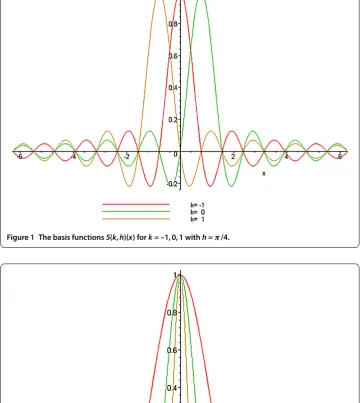
For various values ofk, the sinc basis functionS(k,π/)(x) on the whole real line, –∞<
Figure 1 The basis functionsS(k,h)(x) fork= –1, 0, 1 withh=π/4.
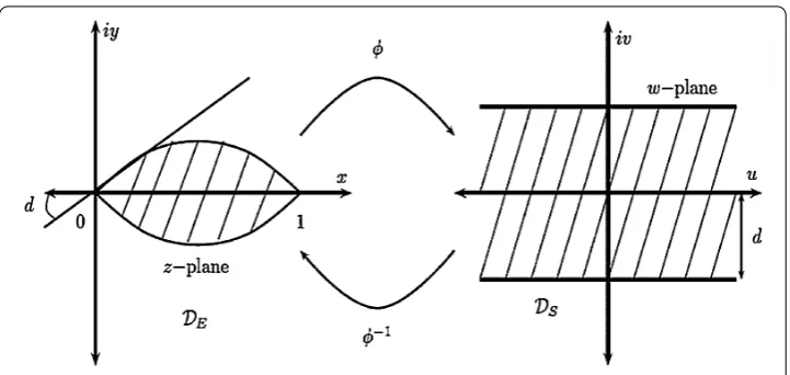
Figure 3 The relationship between the eye-shaped domainDEand the infinite stripDS.
If a functionf(x) is defined over the real line, then forh> the series
C(f,h)(x) =
∞
k=–∞
f(kh)sinc
x–kh h
(.)
is called the Whittaker cardinal expansion off whenever this series converges. The infinite stripDsof the complexwplane, whered> , is given by
Ds≡
w=u+iv:|v|<d≤π
. (.)
In general, approximations can be constructed for infinite, semi-infinite, and finite inter-vals. Define the function
w=φ(z) =ln
z
–z
(.)
which is a conformal mapping fromDE, the eye-shaped domain in thez-plane, onto the
infinite stripDS, where
DE=z=
x+iy:arg
z
–z
<d≤π
. (.)
This is shown in Figure .
For the sinc-Galerkin method, the basis functions are derived from the composite trans-lated sinc functions:
Sh(z) =S(k,h)(z) =sinc
φ(z) –kh h
(.)
forz∈DE. These are shown in Figure for real values ofx. The functionz=φ–(w) = e
w
+ew is an inverse mapping ofw=φ(z). We may define the range ofφ–on the real line as
=φ–(u)∈DE: –∞<u<∞
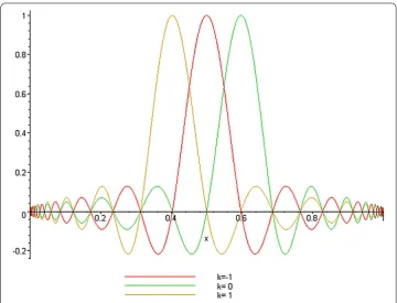
Figure 4 Three adjacent membersS(k,h)◦φ(x) whenk= –1, 0, 1 andh=π8of the mapped sinc basis on the interval (0, 1).
For the evenly spaced nodes{kh}∞k=–∞ on the real line, the image which corresponds to these nodes is denoted by
xk=φ–(kh) = ekh
+ekh. (.)
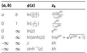
A list of conformal mappings may be found in Table . [].
Definition . LetDEbe a simply connected domain in the complex planeC, and let∂DE
denote the boundary ofDE. Leta,bbe points on∂DEandφbe a conformal mapDEonto DSsuch thatφ(a) = –∞andφ(b) = –∞. If the inverse map ofφis denoted byϕ, define
=φ–(u)∈DE: –∞<u<∞
(.)
andzk=ϕ(kh),k=∓,∓, . . . .
We can use Table to choose convenient conformal map according to boundary condi-tions.
Definition . LetB(DE) be the class of functionsFthat are analytic inDEand satisfy
ψ(L+u)
Table 1 Conformal mappings and nodes for several subintervals ofR
(a,b) φ(z) zk
a b ln(zb––az) a+bekh
1+ekh 0 1 ln(1–zz) ekh
1+ekh 0 ∞ ln(z) ekh
0 ∞ ln(sinh(z)) ln(ekh+√e2kh+ 1)
–∞ ∞ z kh
–∞ ∞ sinh–1(z) kh
where
L=
iy:|y|<d≤π
(.)
and on the boundary ofDEit satisfies
T(F) =
∂DE
F(z)dz<∞. (.)
The proof of following theorems can be found in [].
Theorem . Letbe(, ),F∈B(DE),then for h> sufficiently small,
F(z)dz–h ∞
j=–∞
F(zj)
φ(zj)
= i
∂D
F(z)k(φ,h)(z)
sin(π φ(z)/h) dz≡IF, (.)
where
k(φ,h)z∈∂D=e[iπ φh(z)sgn(Imφ(z))]
z∈∂D=e –πd
h . (.)
For the sinc-Galerkin method, the infinite quadrature rule must be truncated to a finite sum. The following theorem indicates the conditions under which an exponential conver-gence results.
Theorem . If there exist positive constantsα,βand C such that
φF((xx))
≤C
⎧ ⎨ ⎩
e–α|φ(x)|, x∈ψ((–∞,∞)),
e–β|φ(x)|, x∈ψ((,∞)), (.)
then the error bound for the quadrature rule(.)is given by
F(x)dx–h N
j=–N F(xj)
φ(xj)
≤C
e–αNh
α +
e–βNh
β
+|IF|. (.)
The infinite sum in(.)is truncated with the use of(.)to arrive at(.).
Making the selections
h=
πd
N≡
s αN
β +
{
, (.)
whereJ·Kis an integer part of the statement and N is the integer value which specifies the grid size,then
F(x)dx=h N
j=–N F(xj)
φ(xj)
+Oe–(π αdN)/
. (.)
We used Theorems . and . to approximate the integrals that arise in the formulation of the discrete systems corresponding to the second-order boundary value problem.
Theorem . Letφbe a conformal one-to-one map of the simply connected domain DE onto DS.Then
δ()jk =S(j,h)◦φ(x)x=x k=
⎧ ⎨ ⎩
, k=j, , k=j,
(.)
δ()jk =h d dφ
S(j,h)◦φ(x)
x=xk =
⎧ ⎨ ⎩
, k=j,
(–)k–j
(k–j) , k=j,
(.)
δ()jk =h d
dφ
S(j,h)◦φ(x)
x=xk =
⎧ ⎨ ⎩
–π
, k=j, –(–)k–j
(k–j) , k=j.
(.)
3 Convergence analysis
Consider the following problem:
P(x)y+Q(x)y+R(x)NL(y) =F(x) (.)
with Dirichlet-type boundary condition
y(a) = , y(b) = , (.)
whereP,Q,R, andFare analytic onD. We consider sinc approximation by the formula
y(x)≈yN(x) = N
k=–N
ckS(k,h)◦φ(x), (.)
S(k,h) = sin[
π
h(x–kh)] π
h(x–kh)
. (.)
The unknown coefficientsckin Eq. (.) are determined by orthogonalizing the residual
with respect to the sinc basis functions. The Galerkin method enables us to determine the
ckcoefficients by solving the nonlinear system of equations
NLyN–F,S(k,h)◦φ(x)
Letfandfbe analytic functions onD. The inner product in (.) is defined as follows:
f,f=
w(x)f(x)f(x)dx, (.)
wherewis the weight function. For the second-order problems, it is convenient to take []
w(x) =
φ(x). (.)
For Eq. (.), we use the notations (.)-(.) together with the inner product given in (.) [] to get the following approximation formulas:
F(x),S(k,h)◦φ(x)=
w(x)F(x)S(k,h)◦φ(x)dx∼= hwkFk
φk , (.)
R(x)NLy(x),S(k,h)◦φ(x)=
w(x)R(x)NLy(x)S(k,h)◦φ(x)dx
∼=h
wkRk
φk
NL(ck), (.)
Q(x)y(x),S(k,h)◦φ(x)=
w(x)Q(x)y(x)S(k,h)◦φ(x)dx∼=h
wkQk
φk
ck
∼= –hN
j=–N cj
(Qw) j
φj δ
()
kj + (Qw)j
δ()kj
h
, (.)
P(x)y(x),S(k,h)◦φ(x)
=
w(x)P(x)y(x)S(k,h)◦φ(x)dx∼=h
wkPk
φk
ck
∼= –hN
j=–N cj
(Pw) j
φj δ
()
kj +
(Pw)j+(Pw)jφ
j
φj
δ()
kj
h + (Pw)jφ j
δkj()
h
, (.)
where wk =w(xk) etc. The choices h= (πd/αN)/ and w(x) = /φ(x) yield O(N/× e–(πdαN)/) [] accuracy for each of the approximations in (.)-(.).
Using (.), (.)-(.), we obtain a nonlinear system of equations for N+ numbersck.
The nonlinear system with N+ unknowns given in (.) can be expressed by means of matrices. Letm= N+ and letSm,cm,NL(cm) be column vectors defined by
Sm(x) =
⎛ ⎜ ⎜ ⎜ ⎜ ⎝
S–N S–N+
.. . SN ⎞ ⎟ ⎟ ⎟ ⎟
⎠, cm= ⎛ ⎜ ⎜ ⎜ ⎜ ⎝
c–N c–N+
.. . cN ⎞ ⎟ ⎟ ⎟ ⎟
⎠, NL(cm) = ⎛ ⎜ ⎜ ⎜ ⎜ ⎝
NL(c–N) NL(c–N+)
.. .
NL(cN)
LetAm(y) denote a diagonal matrix whose diagonal elements arey(x–N),y(x–N+), . . . ,
y(xN) and non-diagonal elements are zero, and also letIm(),Im()andIm()denote the matrices
Im()=
⎡ ⎢ ⎢ ⎢ ⎢ ⎢ ⎢ ⎢ ⎣ . . . . . . . . . .. . ... ... . .. ... . . . ⎤ ⎥ ⎥ ⎥ ⎥ ⎥ ⎥ ⎥ ⎦ = #
δjk()
$
, (.)
Im()=
⎡ ⎢ ⎢ ⎢ ⎢ ⎢ ⎢ ⎢ ⎣
– . . . N
– . . . –N–
– . . . N–
..
. ... ... . .. ...
–N N– N– . . .
⎤ ⎥ ⎥ ⎥ ⎥ ⎥ ⎥ ⎥ ⎦ = #
δ()jk
$
, (.)
Im()=
⎡ ⎢ ⎢ ⎢ ⎢ ⎢ ⎢ ⎢ ⎣
–π – . . . –(N)
–
π
. . . (N–)
– –
π
. . . –
(N–)
..
. ... ... . .. ...
–(N) (N–) –(N–) . . . –π ⎤ ⎥ ⎥ ⎥ ⎥ ⎥ ⎥ ⎥ ⎦ = #
δjk()
$
. (.)
With these notations, the discrete system in (.) takes the form:
NLyN–F,Sm(k,h)◦φ(x)
=h
Im()Am
(Pw) φ
+
hI
()
mAm
(Pw)+ (Pw)φ/φ+
hI ()
m Am
(Pw)φcm
–h
I()
m Am
(Qw) φ
+
hI
()
mAm(Qw)
cm
+h
I()mAm
Rw
φ
NL(cm)
–hAm Fw
φ. (.)
Theorem . Let c,NL(c)be an m-vector whose jth component is cjand NL(cj)then the system(.)yields the following matrix system whose dimensions are(N+ )×(N+ ):
·c+·NL(c) =Am Fw
φ. (.)
Now we have a nonlinear system with(N+ )equations in the(N+ )unknown coeffi-cients.If we solve(.)with the Newton method(for nonlinear equation systems)by using Maple,we can obtain cjcoefficients for the approximate sinc-Galerkin solution
y(x)≈yN(x) = N
k=–N
4 Examples
In this section, three examples are given to illustrate the performance of the sinc-Galerkin method by solving nonlinear Dirichlet-type boundary value problems. Each of these prob-lems have been chosen to simulate how the solutions change in different zero boundary intervals. In the following examples, the discrete sinc system defined by (.) is used to compute the coefficientscj;j= –N, . . . ,N. The computations are done by the algorithm
which we developed for sinc-Galerkin method by using Maple. The algorithm automati-cally compares the sinc-method to the Newton method. The following examples show that the sinc-Galerkin method is a very efficient and powerful tool for nonlinear Dirichlet-type boundary value problems.
Example . Consider the following nonlinear Dirichlet-type boundary value problem
on the interval [–, ]:
d
dxy(x) +
d
dxy(x) +xy(x)sin
y(x)= –extanx+ x,
y(–) = , y() = .
(.)
We choose the weight function according to [],φ(x) =ln(x–+x),w(x) =φ(x) and by taking
d=π/,h=√
N, xk=
–+ekh
+ekh forN= , , , , the solutions presented in Figure and Table .
Figure 5 The red-colored curve displays the Newton solution and the green one is an approximate solution of Eq. (4.1).
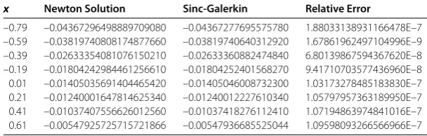
Table 2 The numerical results for the approximate solutions obtained by sinc-Galerkin in comparison with the Newton solutions of Eq. (4.1) forN= 48
x Newton Solution Sinc-Galerkin Relative Error
Figure 6 The red-colored curve displays the Newton solution and the green one is an approximate solution of Eq. (4.2).
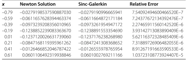
Table 3 The numerical results for the approximate solutions obtained by sinc-Galerkin in comparison with the exact solutions of Eq. (4.2) forN= 32
x Newton Solution Sinc-Galerkin Relative Error
–0.79 –0.0279198537590887030 –0.0279190996665941 7.54092494600466520E–7 –0.59 –0.0611657628394463374 –0.0611664872171184 7.24377672134392476E–7 –0.39 –0.0973239208356010965 –0.0973261954947172 2.27465911560142520E–6 –0.19 –0.1238852239083363670 –0.1238891553354690 3.93142713083890409E–6 0.01 –0.1237120026631739060 –0.1237176238268980 5.62116372328485409E–6 0.21 –0.0847168119395961262 –0.0847241308368652 7.31889726906482055E–6 0.41 –0.0126466852046787422 –0.0126555978765954 8.91267191663590533E–6 0.61 0.0601106492319938846 0.0601002769211166 1.03723108773924407E–5
Example . Let us have the following form of nonlinear Dirichlet-type boundary value problem on the interval [–, ]:
e–x d
dxy(x) +x
d dxy(x) +x
e–y(x)=cos(πx),
y(–) = , y() = ,
(.)
where φ(x) =ln(x–+x), w(x) = φ(x) and by taking d=π/, h= √N, xk = –+e
kh
+ekh forN = , , , we get the solutions presented in Figure and Table .
Example . In this case, we take the problem to be given on the interval [, ]
d dxy(x) +
d dxy(x) –
e–sin(y(x))(y(x)) +y(x) =cos
πxx,
y() = , y() = ,
(.)
where we choseφ(x) =ln(x––x),w(x) =φ(x) and by takingd=π/,h=√N ,xk=+e
kh
+ekh for
N= , , , we get the results presented in Figure and Table .
5 Discussion
Figure 7 The red-colored curve displays the Newton solution and the green one is an approximate solution of Eq. (4.3).
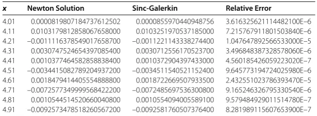
Table 4 The numerical results for the approximate solutions obtained by sinc-Galerkin in comparison with the Newton solutions of Eq. (4.3) forN= 48
x Newton Solution Sinc-Galerkin Relative Error
4.01 0.0000819807184737612502 0.0000855970440948756 3.616325621114482100E–6 4.11 0.0103179812858067658000 0.0103251970537185000 7.215767911801503840E–6 4.21 –0.0011116378549017658700 –0.0011221143338274400 1.047647892566533000E–5 4.31 0.0030747524654397085400 0.0030712556170523700 3.496848387328578060E–6 4.41 0.0010377464582858838400 0.0010372904397433000 4.560185426059223020E–7 4.51 –0.0034415082789204937200 –0.0034511540521152400 9.645773194724025980E–6 4.61 0.0018479414405554888800 0.0018722669507933500 2.432551023786393470E–5 4.71 –0.0072577349999568422200 –0.0072485697536300800 9.165246326795330540E–6 4.81 0.0010544514520660040800 0.0010554094005589100 9.579484929011514780E–7 4.91 –0.0092573478518260567200 –0.0092581760507376400 8.281989115607653900E–7
valid for Dirichlet-type boundary conditions. The order of accuracy used in this paper is
O(N/e–(πdαN)/
). We have used differentNnode points for all figures presented in this paper. Even though the numerical solution looks complex for evenN> node points, Maple handles it very well. In the Appendix, a useful Maple program is given to explain the technique and to show how the same solution can be used for different boundary con-ditions. By using the same program, substitutingNand other parameters (like equations, boundaries), different solutions and graphics can be produced. The total time taken on a . GHz Pentium I processor with Core and GB RAM for producing figures and numerical results is less than seconds.
6 Conclusion
System. Several nonlinear BVPs have been solved by using our technique in less than seconds. All computations and graphical representations have been prepared automati-cally by our algorithm.
Appendix: A computer application of numeric solutions for nonlinear boundary value problems (NBVPs)
We demonstrate below how to solve and simulate for a nonlinear BVP. For example, the following Maple code computes and simulates Example ..
Set all parameters as default values > restart:
For drawing approximation graphics, we must type the following line > with(plots):
A user has to specify with (linalg) for linear algebra operations in Maple > with(linalg):
A user can define the grid point sizeNfor sinc-Galerkin approximation > N:=:
The boundary conditions are given as Eq. (.). > a:=:
> b:=:
> Boundaries:=y(a)=,y(b)=;
Boundaries:=y(a) = ,y(b) = .
P,QandRare the variable coefficients of Eq. (.). In Maple for Eq. (.) they are defined as follows:
> P(x):=;
P(x) := .
> Q(x):=;
Q(x) := .
> R(x):=;
R(x) := .
Fis right side of Eq. (.) > F(x):=cos(Pi*x^)*x;
F(x) :=cosπxx.
> NLPart:=-exp(-sin(y(x)))*y(x)^/(+y(x));
NLy(x)=NLPart:= –e
–sin(y(x))(y(x))
+y(x) .
The main form of Eq. (.)
> Equation:=P(x)*diff(y(x),x$)+Q(x)*diff(y(x),x$)+R(x)*NLPart=F(x);
d
dxy(x) +
d dxy(x) –
e–sin(y(x))(y(x))
+y(x) =cos
πxx.
If the user needs, the main equation can be written in the latex format > latex(Equation);
{\frac {d^{}}{d{x}^{}}}y \left( x \right) +{\frac {d}{dx}}y \left( x \right) -{\frac {{{\rm e}^{-\sin \left( y \left( x \right) \right) }
} \left( y \left( x \right) \right) ^{}}{+y \left( x \right) }}= \cos \left( \pi \,{x}^{} \right) x
In order to compare our method with the Newton interpolation (for nonlinear ODE) method, we first solve Eq. (.) numerically as follows:
> NewtonSolution:=dsolve({Equation,Boundaries},y(x), type=numeric,method=bvp); Prepare the plot of the Newton solution
> PlotNewtonSolution:=odeplot(NewtonSolution,a....b): To defineIm()= [δ()jk ],I
()
m = [δjk()] andI
()
m = [δ()jk ] matrices given in Eqs. (.)-(.), we use
piecewise functions in Maple in the following way: > delta[]:=unapply(piecewise(j=k,,j<>k,),j,k):
> delta[]:=unapply(piecewise(j=k,,j<>k,((-)^(k-j))/(k-j)),j,k):
> delta[]:=unapply(piecewise(j=k,(-Pi^)/,j<>k,-*(-)^(k-j)/(k-j)^),j,k): The parameters for sinc-approximation given []
> d:=Pi/:
> h:=/sqrt(N):
The evenly spaced nodes given (.) and Table are defined as follows: > xk:=unapply((a+b*exp(k*h))/(+exp(k*h)),k);
xk:=k→
+ ekh
+ ekh .
The conformal map in Table for sinc-Galerkin method and its derivatives is computed as follows:
> phi:=unapply(log((x-a)/(b-x)),x);
φ(x) :=x→ln
x– –x
.
> Dphi:=unapply(simplify(diff(phi(x),x)),x): > Dphi:=unapply(simplify(diff(phi(x),x$)),x):
> w:=unapply(/Dphi(x),x):
> Dw:=unapply(simplify(diff(w(x),x$)),x):
> Dw:=unapply(simplify(diff(w(x),x$)),x):
By using sinc-discretization in (.), the matrix system with (N+ )×(N+ ) dimen-sions defined in (.) is obtained by the following iteration:
> MatrixSystem:=[]: for p from -N to N
do
MatrixSystem:=[op(sys), h*(
sum(c[j]*( (/h^)*delta[](p,j)*(
Dphi(xk(j))*subs(x=xk(j),P(x)*w(x)))+ (/h^)*delta[](p,j)*(
(Dphi(xk(j))/Dphi(xk(j)))*subs(x=xk(j),P(x)*w(x))+*subs(x=xk(j), diff(P(x)*w(x),x))) + (/h^)*delta[](p,j)*((subs(x=xk(j),
diff(P(x)*w(x),x$))/Dphi(xk(j))))),j=-N..N)
-sum(c[j]*( (/h^)*delta[](p,j)*(subs(x=xk(j),Q(x)*w(x)))+
(/h^)*delta[](p,j)*(subs(x=xk(j),diff(Q(x)*w(x),x))) /Dphi(xk(j)) ),j=-N..N)
+subs(y(x)=c[p],NLPart)*subs(x=xk(p),w(x)*R(x))/Dphi(xk(p)) -subs(x=xk(p),w(x)*F(x))/Dphi(xk(p)))=]:
od:
If we want to obtain solutions of linear BVPs, we can use the following lines. They can reduce time complexity. Here, the linear solution is given as a comment (“#”).
> #for Linear system > #vars:=seq(c[i],i=-N..N):
> #A,b:=LinearAlgebra[GenerateMatrix](evalf(MatrixSystem),[vars]): > #c:=linsolve(A,b);
In this paper, we want to solve nonlinear problems. Then we usefsolvefunction given by Maple to find unknowncjcoefficients (.)-(.) from nonlinear matrix systems. This
function can solve any nonlinear systems by using the Newton method (for nonlinear equation systems).
> c:=fsolve(evalf(MatrixSystem)):
Finally, we have unknowncjcoefficients for the approximate sinc-Galerkin solution (.)
>ApproximateSol:=unapply(sum(’rhs’(c[j+N+])*sin(Pi*(phi(x)-j*h)/h)/(Pi*(phi(x)-j*h)/h),j=-N..N),x): We define plot of Eq. (.) obtained by the sinc-Galerkin solution
> Sinc-GalerkinPlot:=plot({ApproximateSol(x)},x=a..b,color=green,thickness=): Simulation: Figure , Figure , and Figure are obtained as
> display({Sinc-GalerkinPlot, PlotNewtonSolution }, title =
"Sinc-GalerkinApproximation", labels=["x","y"]);
Enter the number of digits here > Digits := :
Tables , , and are obtained by the following code: > Exact:=[]:Apprx:=[]:Err:=[]:XPoint:=[]:
do
XPoints:=[op(XPoints),s]:
NewtonOutputArray:=[op(Exact),rhs(NewtonSolution (s)[])]: ApprxmOutputArray:=[op(Apprx),evalf(ApproximateSol(s))]:
ErrOutputArray:=[op(Err),evalf(abs(ApproximateSol(s)-rhs(NewtonSolution(s)[])))]: od:
> latex(XPoints);
[., ., ., ., ., ., ., ., ., .]
> latex(NewtonOutputArray);
[., ., –., ., ., –., ., –.,
., –.]
> latex(ApprxmOutputArray);
[., ., –., ., ., –., ., –.,
., –.]
> latex(ErrOutputArray);
[., ., ., ., ., .,
., ., ., .]
Competing interests
The authors declare that they have no competing interests.
Authors’ contributions
AS proposed main idea of the solution schema by using Sinc Method. He developed computer algorithm and worked on theoretical aspect of problem. MK searched the materials about study and compared with other techniques. MAA contributed us with his experience on Nonlinear Approximation methods. MB contributed us with his experience on Nonlinear Approximation methods, suggested us some valuable techniques.
Author details
1Department of Mathematical Engineering, Faculty of Chemical and Metallurgical Engineering, Yildiz Technical University, Davutpasa, ˙Istanbul, 34210, Turkey. 2Department of Mathematics, Faculty of Art and Sciences, Yildiz Technical University, Davutpasa, ˙Istanbul, 34210, Turkey. 3Department of Mathematics, Bilecik University, Bilecik, 11210, Turkey.
Received: 3 August 2012 Accepted: 2 October 2012 Published: 24 October 2012 References
1. Stenger, F: A sinc-Galerkin method of solution of boundary value problems. Math. Comput.33, 85-109 (1979) 2. Stenger, F: Approximations via Whittaker’s cardinal function. J. Approx. Theory17, 222-240 (1976)
3. Whittaker, ET: On the functions which are represented by the expansions of the interpolation theory. Proc. R. Soc. Edinb.35, 181-194 (1915)
4. Whittaker, JM: Interpolation Function Theory. Cambridge Tracts in Mathematics and Mathematical Physics, vol. 33. Cambridge University Press, London (1935)
5. Lund, J: Symmetrization of the sinc-Galerkin method for boundary value problems. Math. Comput.47, 571-588 (1986)
6. Lund, J, Bowers, KL: Sinc Methods for Quadrature and Differential Equations. SIAM, Philadelphia (1992)
7. Lewis, DL, Lund, J, Bowers, KL: The space-time sinc-Galerkin method for parabolic problems. Int. J. Numer. Methods Eng.24, 1629-1644 (1987)
8. McArthur, KM, Bowers, KL, Lund, J: Numerical implementation of the sinc-Galerkin method for second-order hyperbolic equations. Numer. Methods Partial Differ. Equ.3, 169-185 (1987)
9. Bowers, KL, Lund, J: Numerical solution of singular Poisson problems via the sinc-Galerkin method. SIAM J. Numer. Anal.24(1), 36-51 (1987)
10. Lund, J, Bowers, KL, McArthur, KM: Symmetrization of the sinc-Galerkin method with block techniques for elliptic equations. IMA J. Numer. Anal.9, 29-46 (1989)
12. Lybeck, NJ, Bowers, KL: Domain decomposition in conjunction with sinc methods for Poisson’s equation. Numer. Methods Partial Differ. Equ.12, 461-487 (1996)
13. Morlet, AC, Lybeck, NJ, Bowers, KL: The Schwarz alternating sinc domain decomposition method. Appl. Numer. Math. 25, 461-483 (1997)
14. Morlet, AC, Lybeck, NJ, Bowers, KL: Convergence of the sinc overlapping domain decomposition method. Appl. Math. Comput.98, 209-227 (1999)
15. Alonso, N, Bowers, KL: An alternating-direction sinc-Galerkin method for elliptic problems. J. Complex.25, 237-252 (2009)
16. Ng, M: Fast iterative methods for symmetric sinc-Galerkin systems. IMA J. Numer. Anal.19, 357-373 (1999)
17. Ng, M, Bai, Z: A hybrid preconditioner of banded matrix approximation and alternating-direction implicit iteration for symmetric sinc-Galerkin linear systems. Linear Algebra Appl.366, 317-335 (2003)
18. Stenger, F: Numerical Methods Based on Sinc and Analytic Functions. Springer, New York (1993)
19. Koonprasert, S: The sinc-Galerkin method for problems in oceanography. PhD thesis, Montana State University, Bozeman (2003)
20. McArthur, KM, Bowers, KL, Lund, J: The sinc method in multiple space dimensions: model problems. Numer. Math.56, 789-816 (1990)
21. Stenger, F: Numerical methods based on Whittaker cardinal, or sinc functions. SIAM Rev.23, 165-224 (1981) 22. Stenger, F: Summary of sinc numerical methods. J. Comput. Appl. Math.121, 379-420 (2000)
23. Stenger, F, O’Reilly, MJ: Computing solutions to medical problems via sinc convolution. IEEE Trans. Autom. Control43, 843 (1998)
24. Narasimhan, S, Majdalani, J, Stenger, F: A first step in applying the sinc collocation method to the nonlinear Navier Stokes equations. Numer. Heat Transf., Part B, Fundam.41, 447-462 (2002)
25. Mueller, JL, Shores, TS: A new sinc-Galerkin method for convection-diffusion equations with mixed boundary conditions. Comput. Math. Appl.47, 803-822 (2004)
26. El-Gamel, M, Behiry, SH, Hashish, H: Numerical method for the solution of special nonlinear fourth-order boundary value problems. Appl. Math. Comput.145, 717-734 (2003)
27. Lybeck, NJ, Bowers, KL: Sinc methods for domain decomposition. Appl. Math. Comput.75, 4-13 (1996) 28. Zarebnia, M, Sajjadian, M: The sinc-Galerkin method for solving Troesch’s problem. Math. Comput. Model. (2011).
doi:10.1016/j.mcm.2011.11.071
doi:10.1186/1687-2770-2012-117