Numerical investigation of upward air-water annular, slug and bubbly flow regimes

331 *_{Corresponding author}

Email address: kouhikamali@guilan.ac.ir

Numerical investigation of upward air-water annular, slug and bubbly

flow regimes

M. Hassani, M. Bagheri Motlagh, R. Kouhikamali *

Faculty of Mechanical Engineering, University of Guilan, Rasht, Iran

Article info:

Type: Research

Abstract

In this paper, numerical investigation of upward two phase flow of air-water has been studied. Different conditions of flow regimes including annular, wispy annular, slug, churn and bubbly are simulated based on Hewitt and Roberts map, and a good agreement between the experimental data of the map and the numerical simulation has been observed. Accordingly, a proper CFD model in CFD software of Fluent with the required User Defined Function (UDF) has been obtained to simulate two phase flows of fluids with large density ratio in vertical tubes. The simulation is carried out with the volume of fluid (VOF) method and piecewise interface calculation (PLIC) algorithm for tracking the interface for the annular, wispy annular, churn and slug flow regimes and drift flux model for bubbly with proper selection of computational cell and time step sizes. Furthermore, water and air momentum fluxes have been changed and the changes to the flow patterns are studied.

Received: 18/07/2018 Revised: 08/02/2019 Accepted: 15/02/2019 Online: 20/02/2019

Keywords:

Numerical simulation, Two phase flow regimes, Volume of fluid method, Annular,

Slug, Bubbly.

1. Introduction

Many industrial phenomena have been opposed with two phase flow matter. These two phase flows consisting of different regimes can occur in nuclear power generation, refrigeration and oil and gas industry.

Due to the abstruse interaction between phases, phases different density and viscosity, extra turbulence and resulting effective forces, two phase flows have complex dynamics and this issue can direct the phases to have some different configuration and flow patterns. Therefore, different ranges of operating conditions cause the multiphase flows to behave in different ways. The most and reliable research carried out in the

332

also considered that different axial location and different inlet type change the flow patterns. Yang and Shieh [7] found out that beside buoyant force and turbulent fluctuations, the surface tension force also affects the flow regime determination in small tubes. Therefore, the bubble flow and slug to annular flow transitions can happen earlier or later for different fluids with different values of surface tension. Kozulin and Kuznetsov [8] studied the flow regimes and statistical characteristics of two-phase flow of liquid gas in a vertical micro-channel experimentally. Milan et al. [9] investigated the effects of inlet device, flow history and development length on the downward flow regimes of vertical tubes experimentally. They resulted in the dependence of mentioned conditions on the pattern and boundary transitions. Talley et al. [10] also worked on the flow visualization of air-water in horizontal pipes and characterized 27 flow conditions of bubbly, plug, slug, stratified, wavy and annular flow regimes. Chen et al. [11] visualized dispersed bubble, bubbly, confined bubble, slug, churn, annular and mist flow patterns of R134a in a vertical upward tube. They studied the effect of tube diameter on the transition boundaries of flow patterns. Zhang et al. [12] investigated the transition mechanism and criterion of bubbly flow to slug flow. They found out that the transition happens when the velocity ratio reaches its minimum value. Li et al. [13] developed new transition criteria between churn-turbulent and annular flow for downward flow regimes of air-water in large diameter pipes. As one of the industrial applications and importance of two phase flow regimes, Hanifzadeh et al. [14] investigated the effect of air-water flow patterns on the upriser pipe of airlift pump. The regimes they observed were slug, churn and annular, but the best performance of airlift pump was reported in the slug flow regime.

Testing conditions and determinate ranges of important parameters are the biggest disadvantages of the experimental work. Besides, it is sometimes difficult and costly to conduct experiments which probe all relevant phenomena. Therefore, an alternative way is required. With the progressive growth of CFD simulation in recent decades, the deficiencies of

forepassed method can be resolved. Taha and Cui [15] used Volume of Fluid (VOF) multiphase model and simulated slug flow regime. The slugs shape, velocity and distribution of velocity and wall shear stress were also studied. Schepper et al [16], based on Baker chart [1], simulated the gas-liquid and vapor-liquid flow regimes with the use of VOF multiphase model and confirmed that a CFD code can correctly compute the variables of horizontal tube two phase flow. Frank et al. [17] considered interphase momentum transfer due to governing drag and non-drag forces and developed new multiphase flow models for mono- and poly-disperse bubbly flows by Ansys-CFX. The effect of inlet conditions on the bubble formation of air with three liquids of water, octane and semi-octane was studied by CFD [18]. The influences of gas and liquid velocities and inlet gas nozzle size and thickness on the bubble size were also studied. It was concluded that surface tension has a strong effect rather than viscosity and density. Wei et al. [19] used CFD modeling for studying shear stress in a flat sheet membrane bioreactor. For this purpose, they used volume of fluid model. Rahimi et al. [20] investigated air-water slug flow characteristics like its length and pressure drop in the horizontal tube and studied the differences with the flow in inclined pipelines. The impact of inlet conditions on bubble to slug flow transition of air-water flow was studied experimentally and numerically by Gregorc and Zune [21]. Their numerical simulation was in a good agreement with their experimental tests. Pouraria et al. [22] investigated the distribution of phase fraction of water-oil flow in subsea horizontal pipelines and discovered flow patterns for different operating conditions by using the Eulerian-Eulerian approach of CFD simulation.

333 VOF method has been employed for slug, churn,

wispy annular and annular flow regimes, but it is needed to consider drag force for detecting bubbles of the bubbly flow regime. Besides, suitable parameterization of numerical simulation of these regimes has been attained. Accordingly, the influences of changing the inlet conditions on slug, wispy annular and bubbly flow regimes and their pressure drop have been investigated.

2. Mathematical model

Different hydrodynamic conditions of phases can cause them to shape differently beside each other and make various flow patterns. Numerical modeling of these regimes needs to solve the governing equations with a proper numerical approach. In this paper, the volume of fluid (VOF) method of Eulerian-Eulerian approach is employed to model the two phase flow regimes of annular, wispy annular, churn and slug. A model with proper drag force is used to model bubbly flow. These models solve one set of conservation equations and track the interface of moving phases to obtain their volume fractions of each computational cell.

For every phase that is considered, one additional equation is added to compute its volume fraction at computational cells. The quantity of the dispersed phases is solved by the volume fraction equation and the continuous phase volume fraction is obtained from the fact that the cell is occupied by phases with volume fractions sum to unity.

∑ 𝛼𝑞= 1 𝑛

𝑞=1

(1)

where 𝛼𝑞 is the qth volume fraction and n determines the number of phases.

Conservations of mass and momentum are considered as follows, respectively:

𝐷𝜌

𝐷𝑡+ 𝜌∇

⋅

𝑉⃗ = 0 (2) 𝜕

𝜕𝑡(𝜌𝑉⃗ ) + ∇

⋅

(𝜌𝑉⃗ 𝑉⃗ )

= −∇𝑃 + ∇

⋅

[𝜇(∇𝑉⃗ + ∇𝑉⃗ 𝑇)] + 𝜌𝑔

+ 𝐹 (3)

In these equations, V and P are velocity and pressure, respectively. 𝜌 (density) and 𝜇

(dynamic viscosity) are calculated based on the volume fractions of phases in the computational cell. In other words, these governing equations are solved for the mixture fluid by using the following mixture rule:

𝜙 = ∑ 𝛼𝑞𝜙𝑞,

𝑛

𝑞=1

𝜙 = 𝜌 𝑎𝑛𝑑 𝜇 (4)

F is the volumetric force due to surface tension at the interface and is calculated via continuum surface force (CSF) of Brackbill et al. [23]

𝐹 = ∑ 𝜎𝑖𝑗

𝑖,𝑗

𝛼𝑖𝜌𝑖𝜅𝑖∇𝛼𝑖+ 𝛼𝑗𝜌𝑗𝜅𝑗∇𝛼𝑗

0.5(𝜌𝑖+ 𝜌𝑗)

(5)

In which, 𝜅 is the interface curvature calculated as the following:

𝜅𝑞 =

∇𝛼𝑞

|∇𝛼𝑞|

(6)

The extra unknown variable of multiphase flow (volume fraction) and its change along the cells are computed with volume fraction equation:

𝜕𝛼𝑞

𝜕𝑡 + (𝑉𝑞

⋅

∇)𝛼𝑞= 0 (7)

For the bubbly flow regime, the VOF method which considers the phases with the same velocity, causes them to gather and form slugs. Therefore, it is needed to consider the relative velocity and add the relevant terms to the equations. ∇

⋅

(∑ 𝛼𝑞𝜌𝑞𝑉𝑑𝑟,𝑞𝑉𝑑𝑟,𝑞) is added to the right hand side of the momentum equation to designate the relative velocities (𝑉𝑝𝑞) of phases [24].

𝑉𝑑𝑟,𝑞= 𝑉𝑝𝑞− ∑

𝛼𝑘𝜌𝑘

𝜌

𝑝ℎ𝑎𝑠𝑒𝑠𝑛𝑢𝑚𝑏𝑒𝑟

𝑘=1

𝑉𝑞,𝑘 (8)

334

Now, it is needed to capture the position of the interface of the phases. There are different models for interface tracking [25-28]. Among them, the VOF method, due to better mass conservation, simpler use in 3-D geometries and unstructured grid, is attended more. Piecewise linear interface calculation (PLIC) algorithm [29] in VOF model is an accurate technique which models the interface by three steps. In the first step with the help of the amount of phase volume fraction in the main and neighboring cells, the slope of the interface of the phases is determined. The second step consists of modeling interface change caused by the velocity field and inlet mass flux through the face. In the last step, based on the balance of fluxes of the last step, phase volume fraction is computed.

For simulating the turbulences of the problem, the k-ɛ Realizable turbulence model [30] with the enhanced wall function formulation is used. In the current numerical simulation, the commercial CFD software of Fluent 6.3 with the required User Defined Function (UDF) has been used. The pressure implicit with splitting of operators (PISO) is implemented as the pressure-velocity coupling scheme. The PRESTO! scheme interpolates pressure with the discretization method used for momentum equation and turbulent variables is the second-order upwind. The problems are solved with adaptive time step based on constant courant number and average time step size of ∆𝑡 = 5𝑒 − 5𝑠 for slug, ∆𝑡 = 𝑙𝑒 − 6𝑠 for bubbly, churn and annular and ∆𝑡 = 𝑙𝑒 − 7𝑠 for wispy annular flow regime.

The under relaxation factors for solving pressure, density, body force, momentum, turbulent kinetic energy, turbulent specific dissipation rate and turbulent viscosity are considered 0.3, 0.7, 0.7, 0.7, 0.8, 0.8, and 0.8 respectively.

3. Geometrical configuration and operating conditions

A two-dimensional simulation of air-water upward flow is carried out by the VOF method (for annular, wispy annular, churn and slug) and drift flux model (for bubbly flow regime) of

Eulerian-Eulerian approach. The slug, annular, wispy annular, bubbly and churn flow regimes are captured based on Hewitt and Roberts map [3]. This map is created based on low pressure air-water flow and high pressure steam-water in vertical tubes with diameters 1-3 cm with superficial gas and liquid momentum fluxes as vertical and horizontal axes.

Accordingly, a tube with 25.4 mm diameter has been considered. Air and water with special mass fluxes, from distinct inlets, according to the desirable flow regime, at atmospheric pressure and room temperature enter the tube. No slip condition is considered for the wall and with the use of the axis boundary, one half of the tube is modeled in 2-D. Inlet conditions of air and water for considered flow regimes are presented in Table 1.

Table 1. Inlet conditions of air and water for considered flow regimes at the current study.

Flow regime _name Case

Water mass flux (kg/m2_.s)

Air mass flux (kg/m2_.s)

Slug

sa 315.9 1.1

sb 706.5 1.1

sc 999.1 1.1

sd 706.5 0.14

Churn c 315.9 5

Bubbly

ba 29267.2 3.5

bb 91834.4 3.5

bc 91834.4 1.9

bd 91834.4 6.1

Annular aa 315.9 95.1

Wispy annular

waa 9183.4 95.1

wab 29267.2 95.1

wac 91834.4 95.1

wad 91834.4 228.5

335 accurate and places every phase (air volume

fraction of 1 or 0) in every cell.

4. Results and discussion

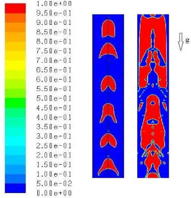
In order to investigate the validity of the numerical procedure for capturing the flow regimes, the bubbly and slug flow regimes of experimental work of Ansari and Azadi [6] have been numerically modeled and shown in Fig. 1.

Fig. 1. Comparison of volume fraction contours of experimental [6] and numerical bubbly (a) and slug (b) flow regimes.

As shown in Fig. 1a, the bubbly flow regime of numerical simulation and the experiment [6] has been compared. Due to transient behavior of the flow, the bubbles in the numerical simulation do not have the same place as the experimental work. But the size of the bubbles seems the same; somewhere with fairly large diameter and somewhere with small one. The volume of the total air bubbles seems the same too. To simulate bubbly flow regime, it is needed to consider the relative velocity between phases. Using the VOF flow regime causes the bubbles to adhere and small slugs to form. As the relative velocity is considered, the slugs are separated. But the commercial CFD codes do not support the two phase flow with surface tension. Therefore, it is

needed to add proper terms of surface tension term to the governing equations of drift flux two phase model.

As in Fig. 1b, the experimental vapor slug inclined a little to the right part of the tube has a circular nose and there are a lot of bubbles in the tail of the slug. While the 2-D symmetrically simulated slug is a little smaller but its form and nose are coincident. The tailing bubbles are adhered and next to each other. This issue can be caused by disability of turbulent model in simulating the turbulence and vortexes of the tail of the air slug. The bubbles in the flow are detected in the numerical visualization but the numbers are lower. Totally, the numerical slug and the two phase flow agree with the experimental work but as explained, there are some defections.

The pressure drop of the bubbly and slug flow regime of the numerical results of Fig. 1 has been computed and is compared with the separated flow model pressure drop [31].

− (𝑑𝑃

𝑑𝑧) = − (

𝑑𝑃 𝑑𝑧)_𝐹+ 𝐺

2 𝑑 𝑑𝑧(

𝑥2𝜈𝑔

𝛼 +

(1−𝑥)2_𝜈 𝑓

1−𝛼 ) +

𝑔𝑠𝑖𝑛θ(𝛼𝜌𝑔+ (1 − 𝛼)𝜌𝑓) (9)

The frictional pressure gradient is obtained from the following relation:

− (𝑑𝑃

𝑑𝑧)_𝐹= − (

𝑑𝑃

𝑑𝑧)_𝑓𝑜𝜙𝑓𝑜

2 ₌

(2𝑓𝑓𝑜_𝐷𝐺2𝜈𝑓) 𝜙𝑓𝑜2 (10)

The two phase frictional multiplier 𝜙𝑓𝑜2 , is calculated based on the Friedel correlation [31].

𝜙𝑓𝑜2 = 𝐴1+

3.24𝐴2𝐴3

𝐹𝑟0.045_𝑊𝑒0.035 (11) where

𝐴1= (1 − 𝑥)2+ 𝑥2

𝜌𝑓𝑓𝑔𝑜

𝜌𝑔𝑓𝑓𝑜

(12)

𝐴2= 𝑥0.78(1 − 𝑥)0.224 (13)

𝐴3= (

𝜌𝑓

𝜌𝑔

)

0.91

(𝜇𝑔

𝜇𝑓

)

0.19

(1 −𝜇𝑔

𝜇𝑓

)

0.7

(14)

𝐹𝑟 = 𝐺

2

𝑔𝐷𝜌2 (15)

𝑊𝑒 =𝐺

2_𝐷

𝜌𝜎 (16)

(a)

336

where x is the gas quality, ffo and fgo are friction

factor based on total flow assumed liquid and gas, respectively, G is the mass velocity and D is the diameter. The second right term of the Eq. (9) is the accelerational pressure gradient which is zero here due to not changing the quality. The third right term of Eq. (9) is the gravitational pressure gradient with θ equals to 90 degrees for vertical tubes.

Table 2 shows the comparison between the calculated pressure drop of the flows [31] with the current numerical results.

Table 2. Comparison of the pressure drop of the flows based on Eq.(9) [31] and the current study.

Pressure drop (Pa) Bubbly flow _{(Fig. 1(a))} Slug flow (Fig. _1(b))

Based on Eq. (9) 1378 725

Present numerical

results 1720 850

4.1. Slug and churn flow regimes

The slug flow regime contains large bubbles with the diameter nearly equal to the tube diameter. They have spherical nose and a flat or protracted tail. Fig. 2 shows four cases related to the slug flow regime, introduced in Table 1. To simulate this regime, air enters from the middle with 7.5 mm length for cases sa, sb and sc and 9 mm for the case sd. Smaller inlet length causes the air to have more speed and tends the regime to have bubbles between slugs or be bubbly slug. It is needed to consider time step size of 5e-5 seconds.

Fig. 2 ) a ( is the case with the lowest amount of water mass flow rate (case sa). As can be seen, the slugs' shape differs slightly, all of them have spherical nose but with different tails.

The lengths of liquid slugs (the length between two air slugs) are approximately equal except for the two last ones. Despite different shapes of slugs' tails, the size of the slugs seems equal. This can be explained with the size of the back liquid slugs which is in the relation with their velocity.

Fig. 2. Slug flow regime for water and air mass flux of 315.9 and 1.1 kg/m2_{.s (a), water and air mass flux}

of 706.5 and 1.1 kg/m2_{.s (b), water and air mass flux}

of 999.1 and 1.1 kg/m2_{.s (c) and water and air mass}

flux of 706.5 and 0.14 kg/m2_{.s (d)}

With increasing water velocity in Fig. 2)b( (case sb), the volume of the slugs has got smaller in comparison with Fig. 2)a(, their shapes are more uniform and their tails are approximately flat. In addition, the total pressure drop of the flow has increased according to Table 3. In sc case (Fig. 2)c(), water velocity is the highest while air mass flow rate is like case sb. It can be observed that not only the sizes of the slugs sizes are smaller but also their numbers have decreased in a special length of the tube. On the other hand, the produced slugs, under the influence of higher water velocity, do not have a continuous shape and there can be seen some water bubbles in among. As Table 3, the increase of the pressure drop is observed with water mass flux increasing. In sd case (Fig. 2)d(), the mass flow rate of water is equal to the case sb, but the air mass flow rate is lower. The decrease in the air mass flow rate causes the slugs to become bigger. Formation of bigger slugs with higher velocity leads to lower numbers in the length and a sharp increase in pressure drop of the flow. In Fig. 1)b(, the slug flow regime of the experimental work in comparison with the current simulation reveals the turbulence defection in capturing the bubbles at the bottom of the slug tail. But in the slugs of Fig. 2, there is no vapor flow below each slug and it seems that in the flow regime with only slugs (not the slugs with bubbles), the turbulence model does not have effective influence.

337

Table 3. Pressure drop of flows of cases sa to sd. Case Water mass flux

(kg/m2_.s)

Air mass flux (kg/m2_.s)

Pressure drop (Pa)

sa 315.9 1.1 310

sb 706.5 1.1 520

sc 999.1 1.1 645

sd 706.5 0.14 1100

In Fig. 3, the resultant changes of increasing air momentum flux to churn part of the map are compared with sa case with the same water momentum flux. The size of the slugs along the cross section and length is sensibly bigger with irregular shape and water in among. The diameters of the slugs are increasing to near the wall and their lengths are extended as a transition between slug and annular flow regimes. In spite of the irregular shape of the churn flow regime, the increase of the air mass flux has reduced the total flow density and decreased the pressure drop to 100 Pa.

4.2. Bubbly flow regime

The bubbly flow regime includes small bubbles dispersed in continuous liquid phase. As shown in Fig. 4, four cases of bubbly flow have been considered. This regime must be solved with small time step near to le-6 seconds. Besides, to capture the bubbles, the quadrilateral cells with 0.25 mm width and length are generated. Otherwise, the convergences would not be obtained.

The bubbly flow regime has to be simulated based on the drift flux two phase flow by which the relative velocity of phases is considered. Besides, the force due to surface tension has to be included in the momentum equation. Without the relative velocity, the bubbles gather and slugs are formed while surface tension prevents the elongated air instead of bubble shape. In the first case (Fig. 4(a)) there seem bubbles of air with different sizes and shapes. Most of the bubbles are elongated. By increasing water momentum flux in case bb, the bubbles get more spherical and their shapes are more uniform. Decrease and increase in air momentum flux in comparison with case bb are shown in Figs. 4c and 4d. Decreasing and increasing the bubble number and size are the respective results. Table

4 compares the pressure drop of the bubbly flow regime.

Fig. 3. Comparison between slug flow regime with water and air mass flux of 315.9 and 1.1 kg/m2_{.s (case}

sa) and churn flow regime with water and air mass flux of 315.9 and 5 kg/m2_.s

Fig. 4. Bubbly flow regime for water and air mass flux of 29267.2 and 3.5 kg/m2_{.s (a), water and air}

mass flux of 91834.4 and 3.5 kg/m2_{.s (b), water and}

air mass flux of 91834.4 and 1.9 kg/m2_{.s (c) and water}

and air mass flux of 91834.4 and 6.1 kg/m2_{.s (d)}

Table 4. Pressure drop of flows of cases ba to bd. Case Water mass flux

(kg/m2_.s)

Air mass flux (kg/m2_.s)

Pressure drop (Pa)

ba 29267.2 3.5 1210

bb 91834.4 3.5 1400

bc 91834.4 1.9 1460

bd 91834.4 6.1 1370

338

According to Table 4, as the gas volume increased in the domain, the less the pressure dropped. More water mass flux in comparison with the slug flow regime has caused more pressure drop in the flow.

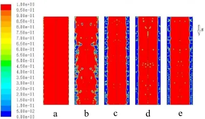
4.3. Annular and wispy-annular flow regimes

In annular flow regime, a liquid film forms on the wall of the tube. The surface of this film can be wavy, but the liquid and gas are completely distinct. In other words, there are no liquid droplets in the core of the flow. But, the wispy annular regime consists of a thick liquid film on the wall which can be full of gas bubbles. On the other hand, the core of the flow can include liquid droplets.

To obtain the annular and wispy annular regimes, the water inlet is placed along the wall and a mean time step value of le-6 and le-7 seconds is used for annular and wispy-annular regimes, respectively.

As can be seen in Fig. 5a, there is a wavy liquid film on the wall. This film is quietly thin and the boundary between liquid and gas is completely distinguishable. Due to high velocity of gas flow, all the annular flows simulated in the current study had the form like Fig. 5a and is not presented. With moving toward the wispy annular part of the map which is caused by increasing liquid velocity, the film on the wall got thicker. Therefore, the pressure drops more from nearly 10 to 140 Pa from case aa to waa. In Fig. 5b (case waa), a completely wavy liquid film can be seen. Big droplets of liquid are separating and there are gas bubbles trapped in the middle of the liquid film. With increasing liquid velocity in the wispy annular flow part (Fig. 5c (case wab)), the waviness of the liquid layer diminishes. The gas bubbles exist in the liquid film consistently and there can be seen more gas bubbles in the core of the flow. Like the changes in Fig. 5c, increases in water velocity cause the surface of the liquid layer more flat. The amount of gas bubbles in the film has got lower but there is a sensible addition in the numbers of the water droplets in the middle of the tube. In Fig. 5e (case wad), mass flow rate of air has increased in comparison with the case 5-wac (Fig. 5d), but the mass flow rate of water

is the same. It can be seen that liquid droplets have decreased but gas bubbles in the film increased. The extra amount of air causes the liquid layer to get wavier too. The pressure drop for Fig. 5c, 5d and 5e is obtained 375, 900 and 800 Pa, respectively.

Fig. 5. Annular flow regime for water and air mass flux of 315.9 and 95.1 kg/m2_{.s (a), wispy annular flow}

regime for water and air mass flux of 9183.4 and 95.1 kg/m2_{.s (b), water and air mass flux of 29267.2 and}

95.1 kg/m2_{.s (c), water and air mass flux of 91834.4}

and 95.1 kg/m2_{.s (d) and water and air mass flux of}

91834.4 and 228.5 kg/m2_{.s (e)}

5. Conclusions

In this study, different flow regimes of air-water (annular, wispy annular, slug, bubbly and churn) based on Hewitt and Roberts map [3] have been investigated in a vertical tube of 25.4 mm diameter. The major purpose of this work is the CFD method which can predict the flow regimes. Therefore, the PLIC algorithm of VOF two phase flow is used to simulate the regimes and tracking the interfaces with proper selection of computational cell and time step sizes, 2-D symmetrical model blinks some asymmetries. It was observed that although the 𝑘 − 𝜀 realizable turbulence model can help predict the total flow, it is weak to simulate the vortexes caused at the tail of the vapor slugs. Besides, for simulating the bubbly flow regime, it is needed to consider the relative velocity of two phases.

By comparing the results with the map of flow in the vertical tube, a good agreement is observed. Also, different conditions of each part in the map are considered.

Changing water and air momentum fluxes cause different results.

339

 In slug flow regime by increasing water velocity, air slugs size gets smaller. Their sizes are approximately equal and increasing water momentum flux decreases their numbers rather than making them smaller to bubble sizes. Increasing the water mass flow rate from 315.9 kg/m2_{.s to 999.1 kg/m}2_{.s with constant air mass}

flux of 1.1 kg/m2_{.s has increased the pressure}

drop more than 50% from 310 to 645 Pa in 0.1 m length. Decreasing the air mass flux of 1.1 kg/m2_{.s to 0.14 kg/m}2_{.s at water mass flux of}

706.5 kg/m2_{.s has also increased the pressure}

drop nearly 50%.

 Wispy annular regime has thicker water layer near the wall. With increasing liquid velocity, the waves of liquid layer decreases and the amounts of liquid droplets in the core flow increase. Increasing gas velocity leads to more waves of the liquid surface and less amounts of liquid droplets.

 Bubble number and size increases with increasing air momentum flux and decreasing water momentum flux values. The pressure drop for 1.9 kg/m2_{.s to 6.1 kg/m}2_{.s air mass flux with}

91834.4 kg/m2_{.s water mass flux has changed}

few from 1460 to 1370 Pa, respectively. While decreasing water mass flux from 91834.3 to 29267.2 kg/m2_{.s decreases the pressure drop}

from 1400 to 1210 Pa.

References

[1] O. Baker, “Simultaneous flow of oil and gas”, oil Gas J., Vol. 53, pp.185-195, (1954).

[2] A. W. Bennett, A. W. Hewitt, H. A. Kearsey, R. K. F. Keeys, P. M. C. Lacey, “Flow visualization studies of boiling at high pressure”, P. I. Mech. Eng., Vol. 180, No. 3, pp. 260-283, (1965).

[3] G. F. Hewitt and D. N. Roberts, “Studies of two-phase flow patterns by simultaneous X-ray and flash photography”, UKAEA Report AERE

M2159, United Kingdom, (1969).

[4] P. J. Waltrich, G. Falcone, J. R. Barbosa, “Axial development of annular, churn and slug flows in a long vertical tube”, Int. J.

Multiphase Flow, Vol. 57, pp.38-48,

(2013).

[5] H. Shaban and S. Tavoularis, “Identification of flow regime in vertical upward air water pipe flow using differential pressure signals and elastic maps”, Int. J. Multiphase Flow, Vol. 61, pp.62-72, (2014).

[6] M. R. Ansari and R. Azadi, “Effect of diameter and axial location on upward gas liquid two-phase flow patterns in intermediate-scale vertical tubes”, Ann. Nucl. Energy, Vol. 94, pp. 530-540, (2016).

[7] C. Y. Yang and C. C. Shieh, “Flow pattern of air–water and two-phase R-134a in small circular tubes”, Int. J. Multiphase Flow, Vol. 27, No. 7, pp. 1163-1177, (2001).

[8] L. A. Kozulin and V. V. Kuznetsov, “Statistical Characteristics of two-phase gas liquid flow in a vertical microchannel”, Journal of Applied Mechanics and Technical Physics, Vol. 52, No. 6, pp. 956-964, (2011).

[9] M. Milan, N. Borhani, J. R., Thome, “Adiabatic vertical downward air-water flow pattem map: Influence of inlet device, flow development length and hysteresis effects”, Int. J. Multiphase Flow, Vol. 56, pp. 126-137, (2013). [10] J. D. Talley, T. Worosz, S. Kim, J. R.

Buchanan, “Characterization of horizontal air-water two-phase flow in a round pipe part I: Flow visualization”, Int. J. Multiphase Flow, Vol. 76, pp. 212-222, (2015).

[11] L. Chen, Y. S. Tian, T. G. Karayiannis, “The effect of tube diameter on vertical two-phase flow regimes in small tubes”,

Int. J. Heat Mass Tran., Vol. 49, No. 21-22, pp.4220-4230, (2006).

[12] M. Zhang, L. m. Pan, P. Ju, X. Yang, M. Ishii, “The mechanism of bubbly to slug flow regime transition in air-water two phase flow: A new transition criterion”,

Int. J. Heat Mass Tran., Vol. 108, Part B, pp.1579-1590, (2017).

340

in large diameter pipes”, Int. J. Heat Mass Tran., Vol. 118, pp. 812-822, (2018). [14] P. Hanafizadeh, S. Ghanbarzadeh, M. H.

Saidi, “Visual technique for detection of gas–liquid two-phase flow regime in the airlift pump”, J. Petrol. Sci. Eng., Vol. 75, No. 3-4, pp. 327-335, (2011).

[15] T. Taha, Z. F. Cui, “CFD modelling of slug flow in vertical tubes”, Chemical Engineering Science, Vol. 61, No. 2, pp. 676-687, (2006).

[16] C. K. De Schepper, G. J. Heynderickx, G. B. Marin, “CFD modeling of all gas– liquid and vapor–liquid flow regimes predicted by the Baker chart”, Chem. Eng. J., Vol. 138, No. 1-3, pp. 349-357, (2008). [17] Th. Frank, P. J. Zwart, E. Krepper, H. M. Prasser, D. Lucas, “Validation of CFD models for mono- and polydisperse air-water two-phase flows in pipes”, Nuclear Engineering and Design, Vol. 238, No. 3, pp. 647-659, (2008).

[18] N. Shao, W. Salman, A. Gavriilidis, P. Angeli, “CFD simulations of the effect of inlet conditions on Taylor flow formation”, International Journal of Heat and Fluid Flow, Vol. 29, No. 6, pp. 1603-1611, (2008).

[19] P. Wei, K. Zhang, W. Gao, L. Kong, R. Field, “CFD modeling of hydrodynamic characteristics of slug bubble flow in a flat sheet membrane bioreactor”, Journal of Membrane Science, Vol. 445, pp. 15-24, (2013).

[20] R. Rahimi, E. Bahrarni far, M. Mazarei Sotoodeh, “The indication of two phase flow pattern and slug characteristics in a pipeline using CFD method”, Gas Processing Journal, Vol. 1, No. 1, pp. 70-87, (2013).

[21] J. Gregorc and I. Žun, “Inlet conditions effect on bubble to slug flow transition in mini-channels”, Chem. Eng. Sci., Vol. 102, pp. 106-120, (2013).

[22] H. Pouraria, J. K. Seo, J. K. Paik, “Numerical modeling of two–phase oil-

water slow patterns in a subsea pipeline”,

Ocean Eng., Vol. 115, pp. 135-148,

(2016).

[23] J. U. Brackbill, D. B. Kothe, C. Zemach, “A Continuum Method for Modeling Surface Tension”, J. Comput. Phys., Vol. 100, No. 2, pp.335-354, (1992).

[24] M. Manninen, V. Taivassalo, S. Kallio,

On the mixture model for multiphase flow, VTT Publications 288, Technical Research Centre of Finland, (1996). [25] G. Tryggvason, B. Bunner, A. Esmaeeli,

D. Juric, N. Al-Rawahi, W. Tauber, J. Han, S. Nas, Y. J. jan, “A Front Tracking Method for the Computations of Multiphase Flow”, J. Comput. Phys., Vol. 169, No. 2, pp.708-759, (2001).

[26] M. Sussman, P. Smereka, S. Osher, “A Level Set Approach for Computing Solutions to Incompressible Two-Phase Flow”, J. Comput. Phys., Vol. 114, No. 1, pp. 146-159, (1994).

[27] D. Jacqmin, “Calculation of Two-Phase Navier–Stokes Flows Using Phase Field Modeling”, J. Comput. Phys., Vol. 155, No. 1, pp. 96-127, (1999).

[28] L. D. Youngs, Time-dependent multi-material flow with large fluid distortion,

in Numerical Methods for Fluid

Dynamics, Academic Press, New York., pp. 273-285, (1982).

[29] J. Li, “Calcul d’interface affin'e par morceaux (piecewise linear interface calculation)”, C.R. Acad. Sci. Paris S’erie

IIb: Paris, Vol. 320, pp. 391-396, (1995). [30] T. H. Shih, W. W. Liou, A. Shabbir, Z.

Yang, J. Zhu, “A new k-epsilon eddy viscosity model for high Reynolds number turbulent Flows - model development and validation”, COMPUT FLUIDS, Vol. 24, No. 3, pp. 227-238, (1995).

[31] J. G. Collier, J. R. Thome, Convective boiling and condensation, 3rd _ed.,

341

How to cite this paper:

M. Hassani, M. Bagheri Motlagh, R. Kouhikamali, “Numerical investigation of upward air-water annular, slug and bubbly flow regimes”, Journal of Computational and Applied Research in Mechanical Engineering, Vol. 9, No. 2, pp. 331-341, (2019).

DOI:

10.22061/jcarme.2019.3893.1453