Temporal stability of electrical conductivity in a sandy soil

Temporal stability of electrical conductivity in a sandy soil**

1_{IFAPA, Las Torres-Tomejil Center, Sevilla-Cazalla km 12.2, 41200 Alcalá del Río, Sevilla, Spain} 2_{Department of Natural Sciences, 291 Campus Drive, Dickinson State University, Dickinson ND 58601, USA} 3_{Department of Agronomy, University of Cordoba, Rabanales Campus, Building L. da Vinci, Madrid Road km 396,}

14071 Córdoba, Spain

4_{Institute for Sustainable Agriculture, CSIC, Avda, Menéndez Pidal s/n, 14080 Córdoba, Spain}

Received January 25, 2016; accepted June 10, 2016

*Corresponding author e-mail: [email protected] **Funding for this work came from the Spanish Ministry of Economy and Competitiveness and FEDER (Grants AGL2012-40128-C03-03 and AGL2015-65036-C3-3-R, MINECO/FEDER, UE)), and from the Junta de Andalucía (P11-AGR-7431). Also support through Ph.D. grant No. 8 (Res. 15/04/2010) by IFAPA is acknowledged).

A b s t r a c t. Understanding of soil spatial variability is needed to delimit areas for precision agriculture. Electromagnetic induction sensors which measure the soil apparent electrical con-ductivity reflect soil spatial variability. The objectives of this work were to see if a temporally stable component could be found in electrical conductivity, and to see if temporal stability informa-tion acquired from several electrical conductivity surveys could be used to better interpret the results of concurrent surveys of electrical conductivity and soil water content. The experimen-tal work was performed in a commercial rainfed olive grove of 6.7 ha in the ‘La Manga’ catchment in SW Spain. Several soil surveys provided gravimetric soil water content and electrical conductivity data. Soil electrical conductivity values were used to spatially delimit three areas in the grove, based on the first principal component, which represented the time-stable domi-nant spatial electrical conductivity pattern and explained 86% of the total electrical conductivity variance. Significant differences in clay, stone and soil water contents were detected between the three areas. Relationships between electrical conductivity and soil water content were modelled with an exponential model. Parameters from the model showed a strong effect of the first prin-cipal component on the relationship between soil water content and electrical conductivity. Overall temporal stability of electrical conductivity reflects soil properties and manifests itself in spatial patterns of soil water content.

K e y w o r d s:apparent electrical conductivity, soil texture, soil water content, spatial variability, temporal stability

© 2016 Institute of Agrophysics, Polish Academy of Sciences INTRODUCTION

Soils are inherently variable in space and time (Brevik

et al., 2016). Knowing this variability helps to establish

proper soil and crop management and to ensure better use of available resources. Recent developments in sensing have led to an increase in surveys of spatial density of soil, and therefore better information regarding soil spatial and temporal variability (Doolittle and Brevik, 2014).

Measurements of apparent electrical conductivity (ECa) provide high spatial data density and allow mapping in great detail. The ECa values reflect various soil properties such as water content, salinity and/or sodicity, clay content, organic matter content, depth to contrasting soil layers, soil compaction, and organic carbon content (Heilig et al.,

2011; Martinez et al., 2009; Saey et al., 2008).

Generally speaking, the more ECa surveys that are carried out in a given area the more information that is col-lected about the spatial variation of soil properties. Several approaches have been proposed to make information from several surveys usable for management decisions. Martinez

et al. (2012) combined multiple electromagnetic induction

Under this assumption, Hedley et al. (2009) delimited three management zones based on a high resolution ECa

survey. Peralta et al. (2013), Pedrera-Parrilla et al. (2014), and Bonfante et al. (2015) have also used EMI to establish management zones. The delineation of management zones within a given field is one of the most common uses of EMI data (Vaudour et al., 2015).

Information from several surveys is also of importance to check whether a variable shows a stable temporal pattern. Temporal stability in ECa data has been demonstrated using Spearman rank correlation (De Caires et al., 2015), correla-tion coefficient between ECa in dry and wet soil conditions (Farahani et al., 2004; Pedrera-Parrilla et al., 2016; Serrano

et al., 2013), and map comparisons (Li et al., 2007). One

effective method of studying temporal stability of spatially and temporally variable soil properties consists in using principal component analysis (PCA) (Vanderlinden et al.,

2012). PCA works by determining principal components (also called empirical orthogonal functions, EOFs) that are dependent only on spatial variables and can be added with temporally dependent coefficients to reproduce the original spatio-temporal data. In cases of well expressed temporal stability, a few principal components explain most of the data variability. Perry and Niemann (2007) used PCs to de- monstrate temporal stability in the Tarrawarra soil mois-ture data set (Australia), and to reconstruct observed soil moisture patterns. Korres et al. (2010) found PCs in spatio- temporal data on surface soil moisture in Cambisol-Stagnosol soils in Germany, where PC patterns were significantly correlated with patterns in soil properties. We are not aware of any applications of PCA to spatio-tempo-ral datasets on soil ECa.

The first objective of this work was to apply PCA to check whether a temporally stable component could be found for ECa in sandy soils in a Mediterranean watershed, where soils are very dry for substantial periods of time during the year. The second objective was to determine if temporal stability information acquired from several ECa

surveys could be used to better interpret results from a sin-gle survey in terms of relationships between ECa and soil water content.

MATERIAL AND METHODS

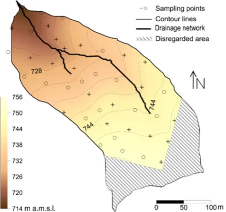
The experimental catchment, ‘La Manga’ (36° 52’ 21” N, 5° 7’ 44”W), is located in Setenil de las Bodegas, SW Spain, and covers 6.7 ha of a rainfed olive grove. The trees were planted in 1995 on a 7 × 7 m grid, with an average tree density of about 200 trees ha-1_{. The mean elevation is 740 m} a.s.l. and the landscape is hilly with a mean slope near 10% (Fig. 1). The soil subgroup is an intergrade between Lithic and Typic Rhodoxeralfs (García del Barrio et al., 1971; Soil Survey Staff, 1999), with a loamy sand texture and a maxi-mum depth of 1.2 m to the calcarenite bedrock. In areas with weakly developed soils, such as the Setenil region, the

rugged relief often leads to partial loss of the topsoil layer (Ibañez et al., 2015; Symeonakis et al., 2014). This is a na- tural process aggravated by certain agricultural practices (eg

tillage) (Gómez et al., 2009; Keesstra et al., 2016; Taguas and Gómez, 2015; Vanwalleghem et al., 2011), leading to outcropping of the bedrock and to the appearance of loca- lised zones where the humus-rich horizon rarely exceeds 0.1 m. The climate is Mediterranean, with a mean annual precipitation of 700 mm, where 75% of the rainfall occurs from October to May. The grove is under minimum til- lage and weeds are controlled with chemical herbicides. The field was tilled in January 2011 and in March 2012. A gully draining the catchment from the SE towards the catchment outlet in the NW separates the two main sub- areas with different slopes and aspects.

Soil profile samples were collected in March 2011 at 41 locations on a pseudo-regular grid (Fig. 1), using a 0.093 m diameter steel cylinder with a percussion drill. Soil samples were taken at intervals of 0.1 m from the surface down to 1.2 m, where possible. The samples were analysed in the laboratory for soil texture, stone content and bulk density (ρ_b). As a result of the shallow soil depth, samples were only available for the first two and three depth intervals at 90 and 52% of the locations, respectively. In order to obtain a spatially consistent soil data set for a homogeneous depth interval, the corresponding values of the first two intervals (0-0.2 m) were averaged. Texture was determined with the hydrometer method (Gee and Or, 2002), stone content by conventional methods (Grossman and Reinsch, 2002), and

ρ_b using the core method (Blake and Hartge, 1986) from

undisturbed samples taken with 250 cm3 _{stainless steel} rings at 21 locations, evenly distributed over the catchment, at depths of 0.05 and 0.15 m, and averaged to obtain ρ_b

for the 0-0.2 m interval. The catchment was sampled on 18 occasions for gravimetric SWC (Fig. 2) at the 0-0.1 and 0.1-0.2 m depth intervals, at the same 41 locations, during two hydrological years (February 2011 – November 2012), using a 0.05 m diameter Edelman auger, and the corre-sponding values of the first two intervals (0-0.2 m) were averaged.

At the same 41 locations where soil properties were cha- racterised, ECa was measured on nine occasions (surveys 9, 10, 11, 12, 14, 15, 16, 17 and 18) using a DUALEM-21S EMI sensor (DUALEM, Milton, Canada). In addition, seven field-wide ECa surveys were conducted (surveys 10, 12, 13, 15, 16, 17 and 18). All the available ECa data were included in the analyses. The DUALEM-21S works at a frequency of 9 kHz and is composed of four receiver coils located at distances of 1, 1.1, 2 and 2.1 m from the transmitter coil and arranged in horizontal-coplanar (H) and perpendicular (P) configurations (Dualem Inc. 2007), allowing simultaneous ECa measurements of four dif-ferent soil volumes with difdif-ferent depths of exploration (DOE). DOE is defined as the depth at which 70% of the

ECa response is obtained from the soil volume above that depth (McNeill, 1980; Callegary et al., 2007). These values are approximately 1.5, 0.5, 3 and 1 m, respectively, for the above mentioned receiver coils.

The EMI soil sensor was placed in a non-metallic sled and pulled by an all-terrain vehicle (ATV) at a speed of 5-10 km h-1_{. The DUALEM-21S was positioned inside}

the sled at a height of 0.075 m above the soil surface as a result of a wear-and-tear plate made of PVC which was mounted underneath the sled to protect it from abrasion by dry soil and stones. The ATV was equipped with a real time kinematic-differential GPS receiver (Trimble, Sunnyvale, CA) and a rugged Allegro-TK6000 field computer (Juniper Systems, Logan, UT) to simultaneously log ECa measure-ments, coordinates and terrain elevation once per second.

The average soil temperature, measured by a 5TE (Decagon Devices, Pullman, WA) sensor network (Espejo

et al., 2014), was used to standardise the ECa values to

a reference temperature of 25ºC (Sheets and Hendrickx, 1995). Because slightly negative ECa values were record-ed in some instances, due to the low values measurrecord-ed and their narrow range in this field, ECa data were referenced to zero, after temperature correction, by subtracting the minimum ECa value from every ECa value. GPS coor-dinates were registered in WGS84 and transformed to the UTM projection ETRS89 datum 30N, with the software Utm9e-200803 (Núñez-Maderal, 2008). The ECa data were filtered to remove possible outliers using the approach pro-posed by Simpson (2009), and interpolated using ordinary point kriging (Goovaerts, 1997) to create maps for the ECa

signal with a DOE of approximately 1.5 m. The interpo-lated maps (1 × 1 m) for the 7 ECa catchment-wide surveys were computed using the Vesper software package (Whelan

et al., 2002). All the variables were interpolated using

ordinary kriging.

The spatial representativeness of each individual ECa

map was characterised by quartiles. First (Q1) and third (Q3) quartiles were calculated in order to delineate three zones (Z1, Z2 and Z3) in the field and to group the 41 sampling locations according to this classification: Z1, locations with ECa < Q1; Z2, locations with ECa > Q3; and Z3, locations with ECa outside the data range for Z1 and Z2. Therefore, for each individual ECa map the field was classified based on quartiles (Z1, Z2 and Z3). An analysis of variance (ANOVA) was performed to check whether differences in measured soil data among the dif-ferent zones were significant. Next a PCA was performed using Matlab (version R2009b, The Mathworks Inc., USA). This transformation consists of inferring independent linear combinations of the analysed variables (here ECa measured on different dates) which are called principle components (PC). The first PC explains the largest proportion of the total variance in the data and represents, in this case, the dominant spatial ECa pattern (Malinowski, 1991). A PCA for the 7 ECa maps was calculated to obtain the dominant spatial pattern of ECa. Based on the spatial distribution of the first PC, the 41 sampling locations were then grouped into three new classes (C1, C2 and C3) based on the first PC

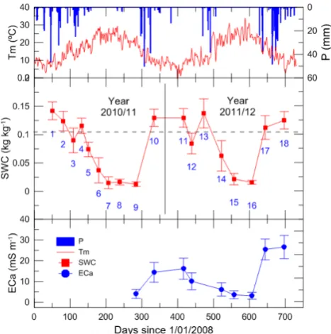
Fig. 2. Temporal evolution of temperature (T, Cº), precipitation (P, mm), mean soil water content (SWC, kg kg-1_{) and mean}

appar-ent electrical conductivity (ECa, mS m-1_{) for hydrological years}

quartiles. After that the stability of the quartile based classi-fication was evaluated. The spatial classiclassi-fications obtained from individual ECa maps were compared with the spatial classification based on the first PC.

An exponential model was fitted to the relationship between the nine ECa and SWC surveys for each sampling location i:

,) (

exp i

i=a bSWC

ECa where: a and b are fitting parameters, the subindex i (i=1,

2, 3…41) represents the soil sampling location, SWC is the soil water content in kg kg-1 _{and ECa is the apparent} electri-cal conductivity in mS m-1_{. To quantify the precision of the} fit, the coefficient of determination (R2_{) and the root mean} squared error (RMSE) between measured (ECa_m) and esti-mated (ECa_e) values were used.

The values of the fitting parameters were checked for significant differences between the three classified areas (C1, C2 and C3) and related to the first PC in order to fit a simple model to interpret the SWC distribution through the time-stable dominant spatial ECa pattern.

RESULTS

Soil texture at the site was dominated by a high and spa-tially uniform (CV = 5%) sand content. Averaged values for clay and stone content were 18 and 7%, with a standard de- viation of 2.5 and 6%, respectively. The average ρ_b value was 1.76 Mg m-3_{, and standard deviation for the field was} 0.10 Mg m-3_{; ρ}

b variations of this level are unlikely to signi-

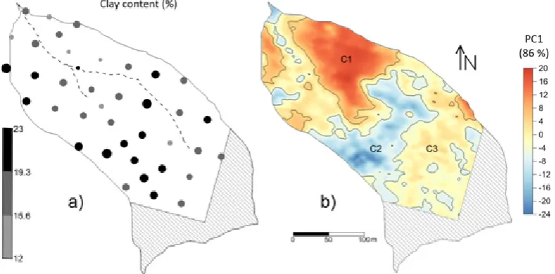
ficantly influence the ECa readings (Brevik and Fenton, 2004). Stone content showed great spatial variability across the catchment, with higher stone contents occurring mainly on the south facing slopes, in the northern part of the catch-ment (Fig. 1). The spatial distribution of averaged clay

content is given as a location map (Fig. 3a). The lowest clay content was found in the N part of the catchment, while in the SE part an area with higher clay content can be seen, as well as in a N-S fringe in the central part of the catch-ment. In the south facing area, the combined occurrence of the highest stone and the lowest clay contents is indica-tive of the great intensity of soil erosive processes in this area (Fig. 1).

Point measurements generated distinctly different ranges of SWCs during dry and wet periods (Fig. 2). Mean topsoil SWCs near or below 0.02 kg kg-1 _were common-ly found during summer (surveys 9, 15 and 16) and were overall associated with the highest CV, ranging from 31 to 50%. Mean SWCs over 0.11 kg kg-1 _{were observed during} wet periods (surveys 10, 11, 13, 17 and 18) and correspond-ed with the smallest CVs, ranging from 11 to 19%. Surveys 12 and 14 showed intermediate mean SWC values and CVs. Descriptive statistics of the nine ECa surveys revealed that surveys 17 and 18 had the highest mean ECa (Fig. 2) and the lowest CV (20%). An intermediate mean ECa and

CV was found for surveys 10, 11 and 12, while surveys 9, 14, 15 and 16 presented the lowest mean ECa and the high-est CV (50%), corresponding to dry soil conditions. The relationships between ECa and SWC data for each sam-pling location showed strong and statistically significant (p<0.005) correlations, with R2 _{values ranging from 0.45 to} 0.94 and a maximum RMSE of 11.5.

Descriptive statistics for the seven ECa maps also showed that surveys 17 and 18 had the highest mean ECa

and the lowest CV, surveys 10, 12 and 13 had an inter- mediate mean ECa and CV, while surveys 15 and 16 pre-sented the lowest mean ECa, corresponding to dry soil conditions. Results from the spatial representativeness analysis of each individual ECa map (Table 1) indicated

significant differences between the zones for clay and stone content, while no significant differences were found for ρ_b. Clay content had significantly lower average values in Z1 as compared to Z2 and Z3 in five surveys, and significantly lower clay contents in Z1 as compared to Z2 in surveys 15 and 16. Average stone content values were significant-ly higher in Z1 as compared to Z2 in surveys 12 and 15. Nevertheless, average SWCs were only lower in Z1 than in Z2 and Z3 in survey 12. Surveys 15 and 16 were char-acterised by low SWCs, while survey 12 had intermediate to high SWCs. Therefore, when the SWC does not hamper the straightforward interpretation of clay and stone con-tent, ECa is a tool to spatially classify these soil properties. Intermediate SWCs are required in this eroded and stony soil to distinguish significantly different zones.

Results from the PCA showed that the first PC accounted for 86% of the total variance of spatial soil ECa. Therefore, the first PC was considered as the time-stable dominant spatial pattern of ECa(Fig. 3b). The first and third quar-tiles, -5.2 and 4.5 respectively, were used to group the 41 sampling locations in the following classes: C1, locations with PC1 < -5.2; C3, locations with PC1 > 4.5; and C2, locations with PC1 outside the data range for C1 and C2.

Evaluation of the quartile based spatial classifications for the 7 ECa maps (Table 2) indicated that classifications of Z1 and Z3 obtained from those single surveys were close to the spatial classification based on the first PC at field averaged SWCs > 0.11 kg kg-1_{. Spatial classifications of Z2} differed from C2 for the 7 individual ECa maps, as com-pared to Z1 and Z2. Spatial classification (Z1, Z2 and Z3) of survey 10 showed the best overlap with spatial classifi-cation based on the first PC (C1, C2 and C3). The soil was surveyed in October, once the first rainfalls were recorded after the characteristic dry Mediterranean summer (Fig. 2). Overall, the percentage of locations included in Z1 for the corresponding C1 was 87%, the percentage of Z2 in C2 was 69%, and the percentage of Z3 included in C3 was 81%. Percentages of locations for Z1 and Z3 in C2, and for Z2 in C1 were all lower than 13%. Although, the percentage of locations for Z3 included in C2 was 31%, indicating that this area is more variable in time, probably as a result of the higher clay contents.

Soil properties were substantially different among the quartile base classification of the first PC (C1, C2 and C3). The ANOVA test indicated significant differences (p<0.05) for clay and stone content, and no differences for

T a b l e 1. Mean and standard deviation for clay and stone contents (%) and soil water content (SWC, kg kg-1_{) for the delimited zones}

(Z1, Z2 and Z3)

Soil property

Survey

10 12 13 15 16 17 18

Clay Z1 15.54±2.38(b) 15.54±2.38(b) 15.54±2.38(c) 15.54±2.38(b) 16.45±2.45(b) 15.56±1.98(b) 15.75±2.34(b) Z2 19.50±1.96(a) 19.66±2.11(a) 19.85±1.75(b) 19.85±1.75(ab) 19.20±2.41(ab) 19.79±1.70(a) 19.14±1.57(a) Z3 17.76±1.80(a) 17.84±1.97(a) 17.82±1.84(a) 17.82±1.85(a) 17.84±2.03(a) 18.15±1.80(a) 18.25±2.28(a) Stone Z1 10.34±6.23(a) 10.34±6.23(a) 10.34±6.23(a) 10.00±5.63(a) 9.43±5.93(a) 9.57±5.88(a) 10.75±6.01(a) Z2 4.69±5.59(a) 3.61±4.65(ab) 4.48±5.77(a) 3.48±4.17(ab) 7.16±7.01(a) 5.28±5.83(a) 4.74±6.29(a) Z3 8.01±6.17(a) 8.34±6.22(b) 7.62±6.05(a) 8.14±6.72(b) 6.19±5.86(a) 7.28±6.57(a) 7.11±5.77(a) SWC Z1 0.12±0.01 (a) 0.07±0.02 (b) 0.13±0.03 (a) 0.02±0.01 (a) 0.013± 0(a) 0.11±0.03(a) 0.12±0.01(a) Z2 0.13±0.02 (a) 0.09±0.02 (a) 0.14±0.02 (a) 0.02±0.01 (a) 0.017± 0(a) 0.12±0.01(a) 0.13±0.01(a) Z3 0.12±0.01 (a) 0.09± 0(a) 0.13±0.02 (a) 0.02±0.01 (a) 0.016± 0(a) 0.11± 0(a) 0.12±0.01(a) Different letters indicate significant differences (p<0.05) between means of delimited zones.

T a b l e 2. Representativeness of the quartile based classification for the delimited zones (Z1, Z2 and Z3) of every survey and the delimited classes (C1, C2 and C3). Cells represent the number of locations of each zone included in each class, for every survey

Classes Survey

10 12 13 15 16 17 18

C1 9/10 9/10 9/10 8/10 8/10 8/10 10/10

C2 14/15 10/15 11/15 7/15 8/15 12/15 10/15

ρ_b among the classes (Table 1). Class C2 showed significant-ly higher clay contents (19.33 ± 2%), causing significantsignificant-ly higher ECa values in this class as compared to C1 and C3. Stone content was significantly higher in C1 (10.75 ± 6%), where the lowest ECa values were found. Significant dif-ferences for SWC among the classes were only detected for survey 16, C2 showed significantly higher SWCs (0.018 ± 0.004 kg kg-1_{). This may be, however, the result of a small} magnitude of SWC variation.

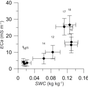
Based on the results from the averaged relationships between SWC and ECa (Fig. 4), an exponential model was fitted for each sampling location using the data from the nine different surveys. Descriptive statistics for the fitting parameters a and b showed averaged values of 3.8 and 14.2, respectively. Parameter a doubled the CV and showed half the range of parameter b. The ANOVA test indicated that parameter a was significantly smaller in C1 as compared to C2 and C3. For parameter b no significant differences were found between the classes. Therfore, parameter a might be related to the soil properties that control the first PC pattern and classification, which is mainly the ECa. Parameter a

showed lower values in the northern part of the catchment, in the area with low clay and high stone contents. Although

the explored soil volumes for the ECa and topsoil mea- surements differed by several orders of magnitude and no strong correlations were expected, the relationship between the ECa and SWC data for each sampling location showed a maximum RMSE of 11.5 and a range of 0.45-0.94 for R2_. These results showed clearly that these topsoil properties influence the SWC and ECa relationships; as significant dif-ferences between the classes were found for the studied soil properties and for the adjusted parameters.

The relationship between the first PC and parameter a

was further analysed to interpret the link between the first PC and the exponential SWC – ECa relationships (Fig. 5). As expected, an inverse relationship was obtained between parameters a and b. An inverse linear relationship was found between a and PC1 (R2 _{= 0.62), indicating that the} lower PC1 was, the smaller the ECa value when the SWC

reached its maximum. The particular established relation-ship could be used to interpret SWC distributions through

ECa measurements.

DISCUSSION

The ECa exhibited a strong temporal stability in this work. A single first PC was able to explain 86% of the spa-tial variability. This percentage of explained variability was larger than analogous values obtained in applications of PCA to soil water contents in previous studies. Korres et al.

(2010) reported that their analysis resulted in one signifi-cant spatial structure (first PC) which explained 57.5% of the spatial variability connected to soil properties and topo- graphy. Similarly, Perry and Niemann (2007) found that the first PC explained about 55% of the spatial variance in soil water contents. One possible reason for this is that the variability of ECa during dry spells is mostly controlled by clay content which is obviously a spatially stable soil pro- perty. The high percentage of explained variability makes the first PC a promising variable to define management zones and predict spatial distribution of soil and crop pro- perties, such as soil water content or yield. Other metrics of temporal stability also have high values. In particular, computation of correlations between ECa measured at the

Fig. 4. Relationship between spatially averaged soil water content (SWC, kg kg-1_{) and apparent electrical conductivity (ECa, mS m}-1_). Error bars represent standard deviations.

Fig. 5. a) Relationship between parameters a and b, and b) relationship between parameter a and first principal component (PC1) for classes C1, C2 and C3. The result of a joint linear regression for the three classes is shown.

SWC (kg kg-1₎

ECa

(

mS m

same location in two different surveys, as suggested by de Caires et al. (2015) and Serrano et al. (2013), provided values of the correlation coefficient (R) from 0.75 to 0.97 in this work (data not shown).

Spatial scales of ECa and SWC measurements differed by orders of magnitude. Besides, the DOE of the ECa

measurements was larger than the soil depth for which water content was measured. Nevertheless, strong correla-tions were observed between ECa and SWC. One possible reason may be the correlative relationships between ECa

measured with different coil configurations. For example, R between the different ECa signals and the selected one (1.5 m DOE) ranged from 0.75 to 0.95, indicating strong and significant (p<0.05) relationships for all survey dates (data not shown).

Relationships between averaged ECa and SWC values followed the exponential model; this type of relation-ship was observed in earlier works (Celano et al., 2011; McCutcheon et al., 2006; Mishra et al., 2014). This expo-nential relationship held at SWCs below 0.11 kg kg-1_, but was not applicable at higher water contents, possibly because of the presence of complex vertical distributions of soil water content in the wet soil. The coefficients in the exponential relationship between ECa and water content at each sampling location varied with the first PC value. These findings indicate that no unique relationship existed between ECa and SWC for the entire study field, as noted by Islam et al. (2011), Pedrera-Parrilla et al. (2014), and Robinson et al. (2009).

The spatial pattern of ECa, represented by the first PC, was significantly related with soil properties in this work. In previous studies, Jawson et al. (2007) demonstrated a relationship between soil texture and the spatial and tem-poral variation in large-scale soil moisture patterns using PCA. Qiu et al. (2014) analysed the soil moisture variabili-ty of various spatial scales based on PCs, and connected the spatial patterns to topography and soil texture at the studied spatial scales. Our study indicated that the spatial pattern of

ECa was related to clay, stone and soil water content. The lowest clay contents and SWCs, as well as the highest stone content, were located in the area that corresponded to C1. This particular spatial distribution of soil properties led to the lowest ECa values in this area.

Three distinct zones were established in this study. Literature shows that three is the most likely selected num-ber of classes to represent soil spatial variability (Hedley

et al., 2009; Jiang et al., 2012; Li et al., 2013), while other authors defined only two zones (Bonfante et al., 2015, De Caires et al., 2015).

CONCLUSIONS

Temporal stability of electrical conductivity was deter-mined using principal component analysis based on seven electrical conductivity surveys. The first principal

compo-nent, which represented the time-stable dominant spatial electrical conductivity pattern in a sandy soil, was used to delimit three areas (C1, C2 and C3) with similar soil conditions.

1. Clay and stone contents were found to be spatially and significantly different among the classes, while soil water content was only spatially different for surveys at interme-diate soil water contents. Clay content, soil water content and electrical conductivity showed the lowest values in C1, while stone content showed the highest values. No spatial differences were found for bulk density. Overall results indicated strong interactions among the analysed soil pro- perties in this eroded and heterogeneous olive grove.

2. Relationships between averaged soil water content and electrical conductivity values were also explored. A clear exponential relationship between spatially averaged soil water content and electrical conductivity was found, although the relationship became indeterminate for water contents above 0.11 kg kg-1_{. The exponential curve also}

modelled the above mentioned relationship at each sam-pling location.

3. The fitted parameter a showed a strong inverse rela-tionship with the first principal component. Therefore, the fitted inverse relationship between parameter a and the first principal component can be used as a simple model to inter-pret SWC distribution through the time-stable dominant spatial electrical conductivity pattern.

4. These findings show that more than a single valid relationship is needed to fully characterise the entire field, and that physical topsoil properties influence the SWC and ECa relationships.

Conflict of interest: The Authors do not declare con-flict of interest.

REFERENCES

Blake G.R. and Hartge K.H., 1986. Bulk density In: Methods of Soil Analysis: Part 1. Physical and mineralogical methods (Ed. A. Klute). Agronomy SSSA Book Ser. 9. SSSA, Madison, WI, USA.

Bonfante A., Agrillo A., Albrizio R., Basile A., Buonomo R., de Mascellis R., Gambuti A., Giorio P., Guida G., Langella G., Manna P., Minieri L., Moio L., Siani T., and Terribile F., 2015. Functional homogeneous zones (fHZs) in viticultural zoning procedure: an Italian case study on Aglianico vine. Soil, 1, 427-441.

Brevik E.C., Calzolari C., Miller B.A., Pereira P., Kabala C., Baumgarten A., and Jordán A., 2016. Soil mapping, clas-sification, and modeling: history and future directions. Geoderma, 264, 256-274, doi:10.1016/j

Brevik E.C. and Fenton T.E., 2004. The effect of changes in bulk density on soil electrical conductivity as measured with the Geonics EM-38. Soil Surv. Horiz., 45(3), 73-110.

Celano G., Palese A.M., Ciucci A., Martorella E., Vignozzi N., and Xiloyannis C., 2011. Evaluation of soil water content in tilled and cover-cropped olive orchards by the geoelectri-cal technique. Geoderma, 163, 163-170.

De Caires S.A., Wuddivira M.N., and Bekele I., 2015. Spatial analysis for management zone delineation in a humid tropic cocoa plantation. Precis Agric., 16, 129-147.

Doolittle J.A., and Brevik E.C., 2014. The use of electromag-netic induction techniques in soils studies. Geoderma, 223-225, 33-45.

Dualem Inc., 2007. DUALEM-21S user’s manual. Dualem Inc., Milton, Canada.

Espejo A., Giráldez J.V., Vanderlinden K., Taguas E.V., and Pedrera A., 2014. A method for estimating soil water dif-fusivity from moisture profiles and its applications across an experimental catchment. J. Hydrol., 516, 161-168.

Farahani H.J. and Buchleiter G.W., 2004. Temporal stability of soil electrical conductivity in irrigated sandy fields in Colorado. Trans. ASAE, 47(1), 79-90.

García del Barrio I., Malvárez L., and González J.I., 1971.

Mapas provinciales de suelos (Provincial soil maps). Cádiz. Ministerio de Agricultura. Madrid, Spain.

Gee G.W. and Or D., 2002. Particle-size analysis. In: Methods of Soil Analysis. Part 4. Physical Methods (Eds J.H. Dane and G.C. Topp). SSSA Book Ser. 5. SSSA, Madison, WI, USA.

Goovaerts P., 1997. Geostatistics for natural resources evalua-tion. Oxford UniversityPress, Oxford, UK.

Gómez J.A., Guzmán M.G., Giráldez J.V., and Fereres E., 2009. The influence of cover crops and tillage on water and sediment yield and on nutrient, and organic matter losses in an olive orchard on a sandy loam soil. Soil Till. Res., 106, 137-144.

Grossman R.B. and Reinsch T.G., 2002. Bulk density and linear extensibility. In: Methods of Soil Analysis. Part 4. Physical Methods (Eds J.H. Dane and G.C. Topp). SSSA Book Ser. 5. SSSA, Madison, WI, USA.

Hedley C.B. and Yule I.J., 2009. A method for spatial prediction of daily soil water status for precise irrigation scheduling. Agr. Water Manag., 96, 1737-1745.

Heilig J., Kempenich J., Doolittle J., Brevik E.C., and Ulmer M., 2011. Evaluation of electromagnetic induction to char-acterize and map sodium-affected soils in the northern Great Plains. Soil Surv. Horiz., 52, 77-88.

Ibañez J.J., Pérez-Gómez R., Oyonarte C., and Brevik E.C., 2015. Are there arid land soilscapes in southwestern Europe? Land Degrad. Develop., doi:10.1002/ldr.2451.

Islam M.M., Saey T., Meerschman E., De Smedt P., Meeuws F., Van De Vijver E., and Van Meirvenne M., 2011.

Delineating water management zones in a paddy rice field using a Floating Soil Sensing System. Agr. Water Manag., 102, 8-12.

Jawson S.D. and Niemann J.D., 2007. Spatial patterns from EOF analysis of soil moisture at a large scale and their dependence on soil, land-use, and topographic properties. Adv. Water Resour., 30, 366-381.

Jiang H.L., Liu G.S., Liu S.D., Li E.H., Wang R., Yang Y.F., and Hu H.C., 2012. Delineation of site-specific manage-ment zones based on soil properties for a hillside field in central China. Archiv. Agron. Soil Sci., 58, 1075-1090, doi: 10.1080/03650340.2011.570337.

Keesstra S., Pereira P., Novara A., Brevik E.C., Azorin-Molina C., Parras-Alcántara L., Jordán A., and Cerdà A., 2016.

Effects of soil management techniques on soil water ero-sion in apricot orchards. Sci. Total Environ., 551-552, 357-366.

Korres W., Koyama C.N., Fiener P., and Schneider K., 2010.

Analysis of surface soil moisture patterns in agricultural landscapes using empirical orthogonal functions. Hydrol. Earth Syst. Sci., 14, 751-764.

Li Y., Shi Z., and Li F., 2007. Delineation of site-specific man-agement zones based on temporal and spatial variability of soil electrical conductivity. Pedosphere, 17(2), 156-164.

Li Y., Shi Z., Wu H.X., Li F., and Li H.Y., 2013. Definition of management zones for enhancing cultivated land conserva-tion using combined spatial data. Environ. Manag., 52, 92-806.

Malinowski E.R., 1991. Factor Analysis in Chemistry. John Wiley and Sons Press, New York, USA.

Martinez G., Vanderlinden K., Ordoñez R., and Muriel J.L., 2009. Can apparent electrical conductivity improve the spa-tial characterization of soil organic carbon? Vadose Zone J., 8(3), 586-593.

Martinez-García G., Vanderlinden K., Pachepsky Y., Giráldez- Cervera J.V., and Espejo-Pérez A.J., 2012. Estimating topsoil water content of clay soils with data from time-lapse electrical conductivity surveys. Soil Sci., 177(6), 369-376.

McCutcheon M.C., Faharani H.J., Stednick J.D., Buchleiter G.W., and Green T.R., 2006. Effect of soil water on appa- rent soil electrical conductivity and texture relationships in a dryland field. Biosyst. Eng., 94(1), 19-32.

McNeill J.D., 1980. Electromagnetic terrain conductivity mea- surement at low induction numbers.Technical Note TN-6. Geonics Limited. Missisauga, Ontario, Canada.

Mishra R.K. and Padhi J., 2014. Assesing field-scale soil water distribution with electromagnetic induction method. J. Hydrol., 516, 200-209.

Núñez-Maderal E., 2008. Calculadora Geodésica edición espe-cial para la Península Ibérica (Geodesic calculator speespe-cial edition for the Iberian peninsula), Cartesia.org, Spain. http://www.cartesia.org/download.php?op=viewdownload details&lid=172&ttitle=Calculadora_UTM-Geogr% E1ficas_Espa%F1a

Pedrera-Parrilla A., Martínez G., Espejo-Pérez A.J., Gómez J.A., Giráldez J.V., and Vanderlinden K., 2014. Mapping im- paired olive tree development using electromagnetic induc-tion surveys. Plant Soil., 384, 381-400.

Pedrera-Parrilla A., Van De Vijver E., Van Meirvenne M., Espejo Pérez A.J., Giráldez J.V., and Vanderlinden K., 2016. Apparent electrical conductivity measurements in an olive orchard under wet and dry soil conditions: signifi-cance for clay and soil water content mapping. Precis Agric., doi:10.1007/s11119-016-9435-z

Peralta N.R., Costa J.L., Balzarini M., and Angelini H., 2013.

Delineation of management zones with measurements of soil apparent electrical conductivity in the southeastern pampas. Can. J. Soil Sci., 93(2), 205-218.

Qiu J., Mo X., Liu S., and Lin Z., 2014. Exploring spatiotempo-ral patterns and physical controls of soil moisture at various spatial scales. Theor. Appl. Clim., 118, 159-171.

Robinson D.A., Lebron I., Kocar B., Phan K., Sampson M., Crook N., and Fendorf S., 2009. Time-lapse geophysical imaging of soil moisture dynamics in tropical deltaic soils: An aid to interpreting hydrological and geochemical pro-cesses. Water Resour. Res., doi:10.1029/2008WR006984.

Saey T., Simpson D., Vitharana U.W.A., Vermeersch H., Vermang J., and van Meirvenne M., 2008. Reconstructing the paleotopography beneath the loess cover with the aid of an electromagnetic induction sensor. Catena, 74, 58-64.

Serrano J.M., Shahidian S., and Da Silva J.R., 2013. Apparent electrical conductivity in dry versus wet soil conditions in a shallow soil. Precision Agric., 14, 99-114.

Sheets K.R. and Hendrickx J.M.H., 1995. Noninvasive soil water content measurement using electromagnetic induc-tion. Water Resour. Res., 31(10), 2401-2409.

Simpson D., 2009. Geoarchaeological prospection with multi-coil electromagnetic induction sensors. Ph.D. thesis, Dept. Soil Management, Faculty of Bioscience Engineering, Ghent University.

Soil Survey Staff, 1999. Soil taxonomy: A basic system of soil classification for making and interpreting soil surveys. USDA-NRCS Agrc. Hdbk. 436. US Gov. Print. Office, Washington, DC, USA.

Sudduth K.A., Kitchen N.R., Bollero G.A., Bullock D.G., and Wiebold W.J., 2003. Comparison of electromagnetic induction and direct sensing of soil electrical conductivity. Agron. J., 95, 472-482.

Symeonakis E., Karathanasis N., Koukoulas S., and Panagopoulos G., 2014. Monitoring sensitivity to land degradation and desertification with the environmentally sensitive area index: the case of Lesvos Island. Land Degrad. Develop., doi: 10.1002/ldr.2285.

Taguas E.V. and Gómez J.A., 2015. Vulnerability of olive orchards under the current CAP (CommonAgricultural Policy) regulations on soil erosion: a study case in Southern Spain. Land Use Pol., 42, 683-694.

Vanderlinden K., Vereecken H., Hardelauf H., Herbst M., Martinez G., Cosh M.H., and Pachepsky Y.A., 2012.

Temporal stability of soil water contents: A review of data and analyses. Vadose Zone J., doi:10.2136/vzj2011.0178.

Vanwalleghem T., Infante-Amate J., González de Molina M., Soto-Fernández D., and Gómez J.A., 2011. Quantifying the effect of historical soil management on soil erosion rates in Mediterranean olive orchards. Agr. Ecosyst. Environ., 142, 341-351.

Vaudour E., Costantini E., Jones G.V., and Mocali S., 2015.

An overview of the recent approaches to terroir functional modelling, footprinting and zoning. Soil, 1, 287-312.