Models for locations and motions in the solar system
Lena Strömberg
Previously Department of Solid Mechanics, Royal Institute of Technology (KTH), Stockholm, Sweden Email: [email protected]
Models for locations in the solar system are presented. For neighboring planets in the solar system, and for three moons of Jupiter, ratios of orbital angular velocities are presented, and suggestions for the origin are discussed. Ratios close to 2.45 are common, and this may be related to the L-frequency of a non-circular orbit. A resulting angular velocity is derived for a generalized elliptic orbit. For small eccentricities, a linearization gives a harmonic solution. It is notified how certain ratios of tones appear in musical acoustics, and a brief model is outlined. The ratio is also found between wavelengths in Northern Light. Assumptions such that ‘differential-locations’ can be calculated as fix points to an iteration formula, are presented. This gives a Julia Set-fractal.
Keywords: Celestial mechanics, generalized elliptic orbit, L-frequency, angular velocity, ratio, fundamental physical constant, fractal location
INTRODUCTION
Considering the locations of planets and satellites of a primary, the distances vary. Presumably originally, at formation, there were certain laws and after that, the planets migrated to their present positions, governed by other rules. In the present context, data for locations of planets and moons is presented, and possible models will be developed.
In mid-18th century, there was the Titius-Bode model, which gives the locations in a compact format,
in terms a power law with 3 parameters. However, this is not a physical model to obtain the entire field, of planetary locations, such that it is valid also for other solar systems, or moons to a primary. In Strömberg (2014), it was suggested that the locations may be due to a frequency coupling between angular velocities and oscillations.
A statistical consideration, e.g. Maximum Likelihood, Millar (2011) gives, that there are many ways to adjust a formula with 3 parameters such that it fits with the location of about 7-8 planets. Other models are also to be found, cf. Scientific Journals. More recently, there were models based on differential equations, e.g. the Schrödinger equation, and modified Laplace equation, with eigen-values. For satellites, several dynamical models are given in Klemperer and Baker (1957).
The model in Strömberg (2014), gives that a planetary orbit with eccentricity depends on an L-frequency derived with a two-step linearization of the Kepler laws. This was applied to Mercury and gives a non-circular orbit (also denoted generalized elliptic orbit). The path could be compared to an ellipsis where perihelion moves, as considered by e.g. Einstein, however calculated in an entirely different manner. Here, additional results for such an orbit will be discussed in terms of ratios between the L-frequency and the angular velocity of a circular orbit.
The aim here, is to show how the model derived in Strömberg (2014), applies with motions at different scales, in the solar system, and universe.
Relating to a subscale context, it will be notified how such frequency ratios occur in musical acoustics. Especially 2 and 27/12 approximately 1.5, appears to be significant natural constants. Observations of Nordic Light, is considered and the
Vol. 2(2), pp. 062-066, March, 2015. © www.premierpublishers.org, ISSN: XXXX-XXXX
Review
Strömberg L 062
colours will be quantified with a ratio.
Preliminaries to derive fractal locations are presented, and the Julia Set is obtained. Restriction to the real axis is exact. Adopting this concept with linearization and iteration formula, gives that the pattern, of the fractal, is related to the distribution of rotating mass. At a larger scale, it has similarities with picturised models of galaxies in Milky Way.
LOCATIONS OF PLANETS AND MOONS
Consider a possible coupling to neighbouring orbit. In Table 1, the ratios of angular velocities for the planets in the solar system are presented. Data are readily found in e.g. Wikipedia. The first value is the ratio between the sidereal angular velocity of Sun and the orbital angular velocity of Mercury.
Table 1. Ratio between inner and outer angular velocities between neighbouring planets, based on data, c.f. Encyclopedia Britannica.
Planet merc venus earth mars asteroids jupiter saturn uran nept
ratio inner/outer 3.2(ecc) 2.5 1.6 1.9 2.4 2.6 2.5 2.8 1.9
In Strömberg (2014), a secondary frequency, subsequently denoted L-frequency, was derived from a two-step linearization, and a relation between this and coupling ratios was suggested. A possible origin for coupling could be a coupling to the out-of-plane motion of Mercury, which, in turn, is related to the non-constant sidereal angular velocity of Sun. It could be notified that a ratio about 2.5 is common and that 3 occur from Venus to Mars. The ratio 2.45, coincides with the upper bound of the L-frequency 6½, c.f. Strömberg (2014) . Mercury, Mars and some of the asteroids (also
present at the same location as Jupiter), have noncircular orbits, such that dependency of an L-frequency ratio is present.
For three moons of Jupiter, the factor 2 appears as coupling, cf. Table 2.
Table 2. Ratio between angular velocities for moons of Jupiter, based on data, c.f. Encyclopedia Britannica.
Moon Io Europa Ganymede Callisto
orbital period/(d) 1.8 3.6 7.2 17
ratio 2 2 2.4
Ratio 2. The moon Io is geologically active (c.f. e.g. Wikipedia), probably due to large tidal forces. It may be such that the factor 2 is avoided among the planets, due to tidal resonance, which in turn, would result in a non-stable Solar System.
In conclusion, we may state that the factors about 2.5 could emanate from the upper bound for L-frequency-ratio. (It may have been reached by migration outwards, (expansion), since factor 2 is nonstable.)
L-frequency in noncircular orbit
In Strömberg (2014) , a two-step linearization of the Kepler laws, is derived, such that the expression for an orbit reads
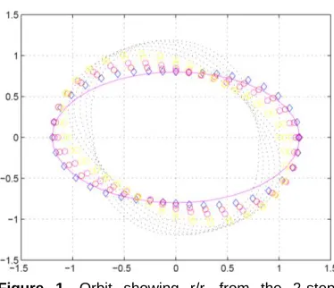
r=r0+re sin(ft) (1)
where r0 is the radius in a circular orbit, re is the eccentricity, f is the L-frequency, f is a factor from the linearization and
is the orbital angular velocity.
Figure 1. Orbit showing r/r0 from the 2-step
linearization with factor f=(4.2)1/2, and eccentricity
re=0.2.
RESULTING ANGULAR VELOCITY, DERIVED FROM 2-STEP LINEARISATION
Proposition: For small eccentricities, or small time increments, the angular velocity is given by
(t)=0 exp(-2(re/r0)sin(f0t)) (2)
Proof. Time differentiation of the Kepler law for angular momentum gives dtln()= -2dtr/r, where dt
denotes time differentiation and ln is the ‘natural’ logarithm.
Insertion of the expression for r, and dtr from r in (1) above, and approximating the denominator to r0, admits an exact
integration. Then, the angular velocity reads as in (2), where0 is an integration constant which corresponds to a circular
orbit.
The angular velocities is shown in the figures, for two cases when the approximation is considered valid, which when eccentricity is large as in Fig 2 is only for a small time interval, (left part of figure). In Fig 3, when the eccentricity is small, the angular velocity is a constant superimposed with a harmonic, for a time interval of arbitrary length.
Script to figure 3 t=[0:.01:2*pi]; ratio=.02
g=exp(-2*ratio*sin(t)); figure(2)
plot(t,g); grid on
0 0.1 0.2 0.3 0.4 0.5 0.6 0.7 0.8 0.9 1 0.5
0.55 0.6 0.65 0.7 0.75 0.8 0.85 0.9 0.95 1
Strömberg L 064
0 1 2 3 4 5 6 7
0.95 0.96 0.97 0.98 0.99 1 1.01 1.02 1.03 1.04 1.05
Figure 3. Resulting angular velocity for a small eccentricity 0.02.
FREQUENCY RATIOS IN MUSICAL ACOUSTICS
Tones on a clarinet with frequency ratios 2 and 27/12 can be obtained with the same valves, but somewhat different
embouchure. The valve to obtain higher tones has a small pipe perpendicular to the opening, and this geometry is not present at a saxophone. Therefore, the saxophone gives the tone 2when this valve is open, whereas the clarinet gives 2*27/12where is the tone at closed valve. Since rotational motion and probably also oscillation, occurs at both smaller
and larger scales, it is possible that the factor 3/2 or 27/12 is a fundamental physical constant related to geometry and
kinematics. This was notified also by Pythagoras; however as it appear not analyzed in details for pipes, c.f. Riedweg (2005).
Model, in brief
Next, a model for generation of the tones in a clarinet will be outlined.
The motion for a particle in a traveling wave according to Falkemo (1980) is rotational with the wave velocity and angular velocity coinciding with the frequency for the wave. Consider a generalization such that the orbit is not circular, but that of a generalized ellipsoidal with radius given by (1). Further, when blowing in the instrument, the traveling wave, is reflected and moves in both direction, such that it is followed and replaced by a stationary wave. The case with ratio 2 is achieved as the tone with half the wave length. The case with ratio
2*27/12 may be determined by the small scale particle velocity, as the primary wave is reflected to opposite phase and
vanishes. Another model for explanation is that the boundary condition changes in some way, related to the wavelength in terms of a rational ratio.
In this context, it can be notified that an approximation of the upper bound 6½, as found as a ratio above, is given by
2*24/12 which is an octave and a major ters. An evaluation gives that the octave and a minor ters is exactly 2.4, and
the octave and a major ters is 2.5. Both these ratios are present among the planets, c.f. Table 1.
NORTHERN LIGHT
Northern light is a phenomenon that occurs close to the earth, and the facts from observations may be readily used.
It is possible that the factor 3/2 is present also in northern light, as the ratio between indigo and green.
The visible light at the night sky has wave length about 370 Nm. The quint (factor 27/12=3/2), from this gives 555
nm, which is close to the wave length observed in Northern Light. In a more detailed description, the maintenance, is due to a (resonance with) ionisation of oxygen, giving 551nm, c.f. Wikipedia.
Figure 5. Northern light with light green and light red at the left.
LOCATIONS RELATED TO FRACTALS
The mechanical laws for gravity in a central motion will be rewritten to an iteration formula for the location of planets, or moons of a primary. For the plane case, a Julia set is obtained for the increment of position vector, r, around a point at equilibrium.
The Kepler law for constant moment of moment of inertia 2r4=const
is expanded about point t0, such that at initial point t0 ,r is assumed linear and dependent on generalized eccentricity, and
next point t1,r has a quadratic dependency but independent of eccentricity. Hereby the equation is modified to read
02r03(r(t1)+ resin(ft1))=02r02r2(t0) (3)
The relation is extended, such thatr is replaced by complex z=x+iy. This is exact at real axis, and at points where r is parallel withrewhich provide that also the eccentricity is considered a complex constant
With the previous step t0indexed by n, and next step n+1, and non-dimensional variablesn=z/z0 , (3) will achieve the
format of an iteration formula:
n+1=n2+c
1 where c1 =-(re/r0)sin(ft1)
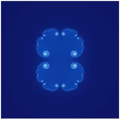
Solving for fix points, a fractal, is obtained, cf. Figure 6.
At left, the fractal when the parameter c1 is real, and the other for complex c1.
Figure 6. Fractals
6a,6b,6c, where c1= 0.285, (0.285+ 0.01i), (0.7 -0.38i).
In Figure 6, the Julia Sets for different values of c1, are shown. The extension to complex xy-plane is assumed to be valid
when Im(c1) is small. These conditions are best met close to real axis, at Fig 6a, and 6b.
Transition to complex analysis implies constraints, such that there are conditions relating the fix points to the constant c1.
A condition consistent with continuity, is that c1 is parallel with r, which implies that the solution is where the line
proportional to c1, intersects the fractal. This condition is met for every line, since a decomposition is arbitrary. However
assuming that c1 evolutes with time is not consistent with the iterations,
and hereby the more consistent solution is where sin(ft1) is constant not dependent on t1, i.e. at vicinity of ft1=/2+mm
Strömberg L 066
It remains to further interpretate how the fractal structure reflects the dynamics of distributed mass, on different scales and levels.
CONCLUSION
With results from Strömberg (2014) , as the point of departure, estimations for locations and other properties was obtained. It was found that the upper bound of L-frequency, may determine the location of a neighbouring orbit.
With some preliminaries, an analytic expression for angular velocity, was derived.
A related remarkable feature is that ratios f, for an L-frequency, appears to be related to harmonics in musical acoustics. Based on this result and the possible occurrence in chaotic celestial mechanics, suppositions on a fundamental physical constant were presented. This could also be the ratio between green and dark night sky in Northern Light.
A fractal structure could be derived from Strömberg (2014), with few assumptions.
However, to manage the implications of the results, there is need for additional analysis. For example, a ‘rotation’ may also be invoked by adding the expansion of as a constant, similar to c1. In general, it was
discussed how the fractal close to the real axis relates to the distribution of rotating mass.
ACKNOWLEDGEMENTS
To my supervisor for valuable discussion and help with the figures and references, and to Johan for stating that ‘the model may be a small two-step for me, but a giant step for mankind’.
REFERENCES
Falkemo C. (1980); Vågenergiboken, Ingenjörsförlaget AB, ISBN 91-7284-080-3, p. 23.
Klemperer W.B. and Baker R.M. (1957); Satellite Librations, Astronautica Acta, 3: 16-27, Springer. Millar RB. (2011); Maximum Likelihood Estimation and Inference , Wiley.
Riedweg C (2005); Pythagoras: His Life, Teaching and Influence, Cornell University Press.
Strömberg L (2014). A model for non-circular orbits derived from a two-step linearisation of the Kepler laws. Journal of Physics and Astronomy Research 1(2): 013-014.
Accepted 20 March, 2015
Citation: Strömberg L (2015). Models for locations and motions in the solar system. Journal of Physics and Astronomy Research, 2(2): 062-066.