Segmentation of Carpal Bones Using Gradient Inverse Coefficient of Variation with Dynamic Programming Method

Vol.9 (2019) No. 1

ISSN: 2088-5334

Segmentation of Carpal Bones Using Gradient Inverse Coefficient

of Variation with Dynamic Programming Method

Sadiah Jantan

, Anuar Mikdad Muad

, Aini Hussain

Electrical and Electronics Section, Universiti Kuala Lumpur Malaysia France Institute, Sect. 14, Jalan Teras Jernang, 43650 Bandar Baru Bangi, Selangor, Malaysia

E-mail: [email protected]

*

Center for Integrated Systems Engineering and Advanced Technologies (INTEGRA), Faculty of Engineering and Built Environment, Universiti Kebangsaan Malaysia, 43600 UKM Bangi, Selangor, Malaysia

E-mail: [email protected]; [email protected]

Abstract— Segmentation of the carpal bones (CBs) especially for children above seven years old is a challenging task in computer

vision mainly because of poor definitions of the bone contours and the occurrence of the partial overlapping of the bones. Although active contour methods are widely employed in image bone segmentation, they are sensitive to initialization and have limitation in segmenting overlapping objects. Thus, there is a need for a robust segmentation method for bone segmentation. This paper presents an automatic active boundary-based segmentation method, gradient inverse coefficient of variation, based on dynamic programming (DP-GICOV) method to segment carpal bones on radiographic images of children age 5 to 8 years old. A mapping procedure is designed based on a priori knowledge about the natural growth and the arrangement of carpal bones in human body. The accuracy of the DP-GICOV is compared qualitatively and quantitatively with the de-regularized level set (DRLS) and multi-scale gradient vector flow (MGVF) on a dataset of 20 images of carpal bones from University of Southern California. The presented method is capable to detect the bone boundaries fast and accurate. Results show that the DP-GICOV is highly accurate especially for overlapping bones, which is more than 85% in many cases, and it requires minimal user’s intervention. This method has produced a promised result in overcoming both issues faced by active contours method; initialization and overlapping objects.

Keywords— carpal bone; segmentation; active contour; gradient inverse coefficient of variation; dynamic programming.

I. INTRODUCTION

Bone age estimation (BAE) is a method of assigning a level of biological maturity to a child. It is widely used in diagnosing heredity diseases and growth disorder. Besides, it is an essential tool in the assessment of children with growth delay and in following response to therapy. BAE is also being used in cases of unregistered child, under-age sports tournaments, juvenile court cases, asylum-seeking children, and forensic practice. In general, the BAE was derived by two methods, comparison of the radiography of hand bones with a reference using Greulich and Pyle atlas [1] or by the numerical scoring system of Tanner-Whitehouse [2]. Both methods are laborious and prone to inter- and intra-observer variability between experienced and inexperienced radiologist. Hence, an automated and consistent method using a computerized BAE (CBAE) method is needed.

There have been many attempts to computerize the BAE procedure ranging from semi-automated in which active shape models are used on the implementation of the TW2

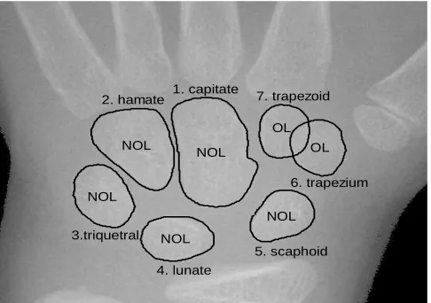
boundaries for all seven carpals bones are highlighted. The numbers (1-7) indicate the most common order of carpal bones appearance based on the natural growth of children. The bones are growth chronologically from bone 1 until bone 7.

Fig. 1 Carpal region of interest indicate non-overlapping bones (1-5) and overlapping bones (6-7) with their ground truth boundary.

Typically, at this age (~7 years old), there are non-overlap (NOL) carpal bones such as capitate, hamate, triquetral, lunate, and scaphoid; and overlaps (OL) bones such as trapezium and trapezoid. The segmentation of hand and wrist anatomical structures is a critical component for CBAE. Features used for describing the bone age are based on boundary, shape, and area can be calculated only after segmentation has been performed. Segmentation for carpal bones is challenging because issues like bone overlapping need to be solved. Various methods such as geodesic active contour with overlap resolution [11], spatial relationship of the non-overlapping and overlapping areas [12], hybrid of local density clustering and gradient-barrier watershed [13], various methodologies to segment a text-based image at various levels of segmentation [14], and morphology analysis [15] are used to segment overlapping or touching objects in different type of images. Active contour methods have become favorites in segmenting carpal bones [16, 17]. However, a significant limitation of the active contour is the inability to detect overlapping objects and sensitive to initialization [11]. Segmentation of overlapping objects in different applications has been previously studied [18-20]. A fusion management algorithm with the cutting line is used to separate the overlapped trapezium and trapezoid [16]. This procedure assumes that the trapezium and trapezoid are not overlapped but appear side by side very carefully. The disadvantage of the cutting line method is that the shape of the trapezium and trapezoid may not be represented accurately.

In boundary detection, dynamic programming (DP) method has been implemented in many applications including in biomedical imaging field applications [21], such as the segmentation of myocardium [22], right [23] and left ventricles [24], breast [25], and lung [26]. The basic idea of DP is to determine the optimum path between two given points, in which those two points are also optimum lying on the path [27]. Therefore, the DP method offers an optimal calculation of global contour with polynomial time [28].

The gradient inverse coefficient of variation (GICOV) [29] is defined as the ratio of average image directional derivatives and its standard deviation along a boundary. Potential carpal bones boundaries possess high GICOV values. DP-GICOV follows the principle of cost function minimization [30]. The combination of GICOV and DP [30] can overcome two main issues faced by the active contour methods: (1) initialization boundary and (2) overlapping region of interest (ROI). In this study, the DP-GICOV method has been implemented on segmenting the carpal bones and then its performance is compared with two other established contouring methods, which are DRLS [33] and MGVF [33].

II. MATERIALS AND METHODS

A. Data

This study is applied to twenty images of carpal bones for male and female children from four ethnic groups, African-American, Asian, Caucasian, and Hispanic from hand radiographs database developed by University of Southern California (USC) (http://ipilab.usc.edu/BAAweb/) [31]. In this study, the range of children age was from 5 to 8 years old. Each image contains overlapping (OV) and non-overlapping (NOV) carpal bones.

B. DP-GICOV

Gradient inverse coefficient of variation (GICOV) measures the ratio of the mean and standard deviation of directional image derivatives over an entire closed contour fitted using active contour techniques to a carpal bone boundary. The directional derivatives are the normal outward directions on contour points [30]. The gradient of the derivative images is computed as in Eq. (1)

(

)

= +

%

x y

g I I (1)

Where I_x= ∂ ∂I x and I_y= ∂ ∂I y. I is the original image. Using directional information of the gradient, the directional gradient is obtained in Eq. (2).

(

)

(

)

cosθ sinθ

= x+ y x + y

g I I sign I I (2)

Where θ is the angle of the radial line taken from a centroid of a two-dimensional closed contour. This centroid can be used as a point of initialization for the closed contouring method.

GICOV score is the ratio of the mean and the variance of the directional gradient, g(v1) at a point v1 on the first radial line through, g(vN) at a point vN on the Nth radial line as given in Eq. (3).

(

)

(

_{( )}

( )

_{( )}

( )

)

2 1

1

1 ,..., ,...,

var ,...,

 

 

=

 

 

N

N

N

mean g v g v

G v v

g v g v

(3)

In order to maximize Eq. (3) using DP [30], this equation is rewritten as given in Eq. (4)

1. capitate

NOL 2. hamate

NOL

3.triquetral NOL

4. lunate NOL

5. scaphoid NOL

6. trapezium OL 7. trapezoid

( )

(

)

( )

(

( )

)







g v g v s

N N

(4)

where s is the noise variance.

The cost function of the active contour is given in Eq. (5).

(

)

(

)

(

)

(

)

(

)

1 1 1 2 2 2 3

1 1 1

, , ; , ; , ; , ; , ; − − = + + + K K N

N N N N N

E v v c E v v c E v v c

E v v c E v v c

(5)

The Eq. (5) is computed using dynamic programming. In Eq. (5) c is the center of the contour, and each cost function is defined in Eq. (6)

( )

(

)

( )

(

)

1 1

2 if ,

otherwise δ +  _{− ≤}  = ∞ 

i i i i

g v cg v D v v

E (6)

where function D(x) measures the distance between point vi to point vi+1, andδ is the distance threshold.

C. Carpal Bones Segmentation

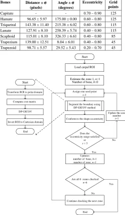
The workflow of the proposed carpal bones segmentation procedure is shown in Fig. 2. Firstly, the orientation of the hand image is corrected [17]. Manual intervention is required to estimate the centroid of the capitate and to initialize the zonal mapping procedure. Here, the intervention is the only input required from users in which a seed point is assigned. Based on the centroid, the carpal region of interest (CROI) is derived containing all the seven carpal bones. Based on [16], six zone boundaries are derived from detecting every carpal bone in a sequential order according to the natural growth of the bones. The designated zone area is typically larger than the expected bone area. Any detected bone boundary that touches the zone boundary is considered invalid. DP-GICOV will only perform the contouring inside the zonal area.

The first zone is derived to ensure that the capitate bone lies approximately at the center of the zone. The rectangular box of zone 1 in Fig. 3(a) is derived sufficiently broad to cover the area of the capitate and avoiding overlapping of lines between the zonal box and capitate boundary. Approximation of the size and location of the zonal box that would fit the capitate bone in all the images in the datasets are used. These approximations are based on heuristic analysis that takes the averages of the size and location of the zonal box from the images in the datasets. In Table 1, the typical values from the capitate centroid to other carpal bones centroids for their distance, angle, eccentricity, and grid points are approximated heuristically from the images in the datasets.

A seed point is assigned at the center of the zone in which the center of the zone is regarded as the centroid of the capitate bone, as shown in Fig. 3(a). The seed point is used to initialize the derivation of the bone boundary. From the seed point, the boundary of the capitate bone is derived using DP-GICOV. The shape of the derived carpal bones is validated according to its shape eccentricity, which is in the range of 0.7–0.9 and shown in Table 1. If the shape eccentricity of the derived bone is not within that range,

more seed numbers will be assigned within proximity of the original seed point to repeat the process of DP-GICOV initialization until the eccentricity of the bone fall within the predetermined range.

TABLEI

MEAN VALUES FOR DISTANCE AND ANGLE, ECCENTRICITY AND GRID POINTS

Bones Distance ± σσσσ

(pixels)

Angle ± σσσσ (degrees)

Eccentricity Grid points

Capitate - - 0.70 – 0.90 125

Hamate 96.65 ± 5.97 175.00 ± 0.00 0.60 – 0.80 125 Triquetral 143.38 ± 11.40 215.38 ± 6.02 0.60 – 0.80 115 Lunate 127.91 ± 8.10 258.39 ± 5.74 0.40 – 0.80 115 Scaphoid 115.01 ± 8.10 326.33 ± 6.61 0.40 – 0.80 85 Trapezium 139.00 ± 12.51 8.04 ± 6.01 0.40 – 0.80 45 Trapezoid 98.71 ± 5.57 29.52 ± 5.43 0.20 – 0.70 45

Continue checking the next zone No

Yes

Yes

No

Update the seed number

s+1

Conform to the shape eccentricity Segment the boundary using

DP-GICOV method

Does the eccentricity range satisfied

or

s = 3

Start

Load carpal ROI

Estimate the zone 1, n=1 Number of bone, b=0

Assign one seed point

s=1

Updates: number of bone, b+1 number of zone, n+1

Are all 6 zones checked

n=6

End Transform ROI to polar domain

Compute cost matrix

Start

End DP-GICOV

Invert ROI to Cartesian domain

Fig. 2 The outline flowchart of the main steps of carpal bones detection using the DP-GICOV segmentation method.

The detection of the subsequent bones follows the general chronological order of the natural growth of the carpal bones, as shown in Fig. 1. Throughout the age from 0 to 18 years old, the growth of the carpal bones is observed to be by the appearance of each carpal bone, one after another, in chronological order. Capitate bone is first developed, followed by hamate, then triquetral, lunate, scaphoid, trapezium and finally trapezoid.

0.6–0.8. This procedure is repeated to find the other bones in zone 3 until zone 6. Fig. 3(b) shows the allocation of all the zones on the carpal bones image. Unlike zone 1-5 that contain only one carpal bone in each zone, zone 6 may contain one or two bones. These two bones are trapezium and trapezoid.

In most cases, trapezium will first to appear then followed by the trapezoid. As the growth of the children continues, these two bones are getting larger until they may appear to be overlapped onto each other. Therefore, the detection of these two bones is more challenging than the other bones. These two bones can be differentiated by referring to the distance and angle to the centroid of the capitate

(a) (b) (c)

Fig. 3 Zone mapping for all carpal bones. (a) Zone 1 - capitate. (b) Zone 2 – hamate, zone 3 – triquetral, zone 4 – lunate, zone 5 – scaphoid, zone 6 – trapezium and trapezoid. (c) Estimated centroid for all the carpal bones.

Typically, bone with a shorter distance and larger angle to the centroid of the capitate is referred to trapezoid. To confirm the existence of trapezium and trapezoid bones, Table 1 is used as a look-up table. The prior knowledge about the distance, angle, and eccentricity of the trapezium and trapezoid assists DP-GICOV to derive the boundaries of these two bones. Fig. 3(c) shows the estimated centroid their standard deviations for all carpal bones.

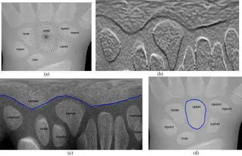
The optimal carpal bones pathfinding using the DP-GICOV method is demonstrated with capitate bone as shown in Fig. 4. Since the carpal bones images have star-shaped boundaries, the optimal boundaries can be determined using polar coordinates. The objective is to find a closed boundary along which the image has uniform edge strength [30]. Fig. 4 illustrate the approach. A center point is chosen as the origin for the polar coordinate system within the image, I, shown in Fig. 4(a) and transform the image into polar coordinates, I’, as shown in Fig. 4(b). The x-axis in the polar image represents the length of the radial line from the centroid to P grid points, and the y-axis represents the angle of the radial line from 0 to 3600. The DP is based on a radial mesh of grid points, with N number of radial lines and P grid points on each line. Therefore, there are PN different possible closed boundaries. Then, the uniform edge strength of I’ is calculated and the optimal boundary is determined as shown in Fig. 4(c). Finally, the detected boundary is transformed back to the Cartesian coordinates, as shown in Fig. 4(d).

III.RESULTS AND DISCUSSIONS

Segmentation results from the proposed DP-GICOV are compared with DRLS [32] and MGVF [33] methods. Manual segmentation performed by two observers is used as ground truth (GT). The segmentation accuracy is measured using the Jaccard index [34]. An analysis is done to determine the optimal number of radial lines, N that can assist DP-GICOV in the segmentation task. The performance

of the DP-GICOV method is tested using 11 different sets of radial lines on capitate, starting from N=50 until N=550 with the increment of 50. As shown in Fig. 5, the method starts to converge and stabilize at 61.2 seconds with N=300, and the Jaccard index is more than 90% and modified Hausdorff distance (MHD) less than 4 pixels. Based on these results, the optimal number of N=300 is chosen for further segmentation tasks. Then, the radius length of the N is chosen based on the average size of the individual bone based on Table 1. Any increment of the number of radial lines would not significantly increase the Jaccard index but merely increase the computational complexity. On the other hand, reducing the number of radial lines may speed up the segmentation time at the expense of segmentation accuracy. Fig. 6 displays boundaries determined using four different values for N, i.e. 100, 200, 300, 350. The GICOV value increases with the increment of N, and the optimum boundary is determined when N=300 with GICOV score

G=5.15.

Both the DRLS and MGVF require human intervention on each carpal bone to initialize the segmentation as shown in red curves in Fig. 7(a) and Fig. 7(b). In contrast, the proposed DP-GICOV does not require initialization on each bone. Only the centroid of the capitate bone that needs to be determined by users. It is therefore reduced the human intervention in the DP-GICOV. Fig. 7(c) shows the result of boundary segmentation of all the carpal bones using only initializing at the centroid of the capitate assisted with 300 radial lines.

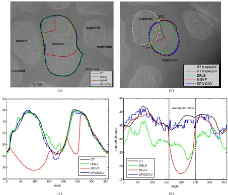
More analyses are focused on the individual NOL bone like capitate and OL bone trapezium, as shown in Fig. 8. The segmentation boundaries derived from DRLS, MGVF, and DP-GICOV are overlaid on the capitate (NOL bone) and trapezium (OL bone) in Fig. 8(a) and Fig. 8(b), respectively. The boundaries of the GT for both bones are used as a benchmark. The centroid distance (CD) shape signatures of

ZONE 2

ZONE 3

ZONE 4

ZONE 5 ZONE 6 ZONE 1

capitate and trapezium are compared against GT. The CD denotes the distances of the boundary points from the centroid of the bone. For capitate bone, the CD shape signature of DP-GICOV followed the GT signature closely as shown in Fig. 8(c). DRLS tended to overestimate the capitate boundary, MGVF has massively underestimated the boundary, while DP-GICOV produced a close estimation of the boundary. For OL bones, the intersection points between

trapezium and trapezoid are at the angles IP1 = 201.4O and

IP2 = 108.2O measured from the centroid of the trapezium. CD shape signature of DP-GICOV for trapezium followed the GT signature closely. Both DRLS and MGVF suffered in the case of OL bones as they underestimated the boundary of the trapezium. Here, the estimation of the boundary for NOL and OL bones using DP-GICOV produced the best estimation close to the GT boundary.

(a) (b)

capitate hamate

triquetral

lunate

scaphoid trapezium

trapezoid

(c) (d)

Fig. 4 (a) carpal bones ROI with 36 radial lines emanating from the capitate centroid (b) cost image after polar transform with radial lines R=300 (c) minimum cost path overlaid on the polar (d) segmented capitate bone boundary overlaid on the Cartesian image.

50 100 150 200 250 300 350 400 450 500 550 0

25 50 75 100

Total number of radial lines, RL

J

ac

c

a

rd

(%

)

13.2s 21.16s

32.5s 41.9s

52.0s

61.2s 71.0s 85.7s 91.8s 112s 149s

0 100 200 300 400 500 6000 5 10 15 20 25 30

M

H

D

(

pi

x

el

s

)

Fig. 5 Determination of the optimal number of radial lines. Fig. 6 Different values of the radial line produce different GICOV scores.

Further analysis is done to determine the accuracy of segmentation techniques under different brightness levels.

The segmentation results using DRLS, MGVF, and DP-GICOV on a different level of brightness are demonstrated

G350=5.89 G300=5.15 G200=4.33 G100=2.77

Angle - RL

R

a

d

iu

s

p

o

in

ts

capitate

hamate

triquetral lunate

scaphoid trapezium

trapezoid

50 100 150 200 250 300 350 20

40 60 80 100 120 140 160 180 200 220

in Fig. 9. The brightness of the three images is low, medium, and high. DP-GICOV produced the best results with the accuracy of more than 80% of the Jaccard index for all the bones in three different brightness conditions. DRLS and MGVF produced less accurate results especially for OL bones such as trapezium and trapezoid. The results suggest that the DP-GICOV is robust in a different level of image brightness and performs well for segmenting the NOL and OL bones.

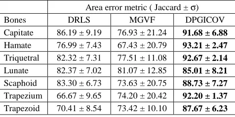
The accuracy assessments for 20 images are presented in Table 2. DP-GICOV produced the best percentage of the Jaccard index. Also, the DP-GICOV technique produced the lowest standard deviations as compared to DRLS and MGVF techniques. The results suggest that the DP-GICOV is the most accurate than that of DRLS and MGVF in segmentation NOL and OL bones.

(a) (b) (c)

Fig. 7 CROI with corresponding segmentation results for all 7 carpal bones using (a) DRLS (b) MGVF and (c) DP-GICOV. The red curves are the initial boundary for DRLS and MGVF methods, the black curves are the GT, and the blue curves are the segmentation results. DP-GICOV does not need an initial boundary, but it needs radial lines.

(a) (b)

(c) (d)

Fig. 8 Bone profile using DRLS, MGVF, and DP-GICOV (a) Segmentation boundaries overlaid on a NOL bone (capitate) (b) Segmentation boundaries overlaid on an OL bone (trapezium) (c) CD shape signatures of a NOL bone (capitate) (d) CD shape signatures of an OL bone (trapezium)

capitate hamate

triquetral

lunate

scaphoid trapezium trapezoid

GT DRLS MGVF DPGICOV

0 50 100 150 200 250 300 350 15

20 25 30 35 40 45

angle

c

e

n

tr

o

id

d

is

ta

n

c

e

overlapped zone

GT DRLS MGVF DPGICOV 0 50 100 150 200 250 300 350

20 30 40 50 60 70 80 90

angle

c

e

n

tr

o

id

d

is

ta

n

c

e

GT DRLS MGVF DPGICOV

capitate hamate

triquetral

lunate

scaphoid trapezium trapezoid capitate

hamate

triquetral

lunate

(a) (b)

(c) (d)

(e) (f)

Fig. 9 Segmentation accuracy at the various level of brightness. (a) Low brightness and (b) its Jaccard index for each bone. (c) Medium brightness and (d) its Jaccard index. (e) High brightness and (f) its Jaccard index.

TABLEII

THE MEAN AND STANDARD DEVIATION OF JACCARD INDEX ACCURACY FROM 20 IMAGES BASED ON INDIVIDUAL CARPAL BONES.

IV.CONCLUSIONS

This paper presents carpal bones boundary detection using DP-GICOV that is implemented in each of the mapping zones. The mapping zone is generated based on a chronological order according to the natural growth of children. This approach overcomes two common issues faced by other segmentation techniques, (1) initialization requirement for active contour and (2) overlapping bones. Also, DP-GICOV can minimize user’s intervention during the initializing process. Only one user input is required to segment all the seven carpal bones. Compared to DRLS and MGVF, DP-GICOV can closely estimate the boundary of the carpal bones, thus producing the most accurate results in a different level of brightness especially for overlapping

bones with the accuracy more than 85%. For future work, we would focus on the estimation of child’s age based upon the growth of the carpal bones, in terms of the number of bones, size, and spatial orientation of the bones.

REFERENCES

[1] W. W. Greulich and S. I. Pyle, Radiographic Atlas of Skeletal Development of Hand and Wrist, 2nd ed. Stanford California USA: Stanford University Press, 1959.

[2] J. M. Tanner and R. H. Whitehouse, Assessment of Skeletal Maturity and Prediction of Adult Height (TW2 Method). London, UK: Academic Press, 1975.

[3] M. Niemeijer, "Automating skeletal age assessment," Master Institute of Information and Computing Sciences, Universiteit Utrecht, 2002. [4] G. W. Gross, J. M. Bonne, and D. M. Bishop, "Pediatric skeletal age:

determination with neural networks," Radiology, vol. 195, pp. 689-695, 1995.

[5] E. Pietka, A. Gertych, and K. Witko, "Informatics infrastructure of the CAD system," Comput. Med. Imaging Graph., vol. 29, pp. 157-169, 2005.

[6] C. W. Hsieh, T. L. Jong, and C. M. Tiu, "Bone age estimation based on phalanx information with fuzzy constrain of carpals," Med. Biol. Eng. Comput., vol. 45, pp. 283-295, 2007.

[7] J. Liu, J. Qi, Z. liu, Q. Ning, and X. Luo, "Automatic bone age assessment based on intelligent algorithms and comparison with TW3 method," Comp. Med. Imaging and Graph., vol. 32, pp. 678-684, 2008.

[8] A. Tristan-Vega and J. I. Arribas, "A radius and ulna TW3 bone age assessment system," IEEE Trans. Biomed. Eng., vol. 55, pp. 1463-1476, 2008.

[9] M. Rucci, G. Coppini, I. Nicoletti, D. Chell, and G. Valli, "Automatic analysis of hand radiographs for the assessment of skeletal age: a subsymbolic approach," Comput Biomed Res, vol. 28, pp. 239-256, 1995.

[10] D. S. O'Keefe, "Denoising of Carpal Bones for Computerised Assessment of Bone Age," Doctor of Philosophy, Dept of Electrical and Computer Engineering, Univ. of Canterbury, Christchurch, New Zealand, 2010.

[11] H. Fatakwala, J. Xu, A. Basavanhally, G. Bhanot, S. Ganesan, M. Feldman, J. E. Tomaszewski and A. Madabushi, , "Expectation-maximization-driven geodesic active contour with overlap resolution (EMaGACOR): Application to lymphocyte segmentation on breast cancer histopathology," IEEE Trans. Biomed. Eng., vol. 57, pp. 1676-1689, 2010.

[12] J. Zhang, Z. Hu, G. Han, and X. He, "Segmentation of overlapping cells in cervical smears based on spatial relationship and overlapping translucency light transmission model," Procedia Tech, vol. 60, pp. 286–295, 2016.

[13] H. Yang and N. Ahuja, "Automatic segmentation of granular objects in images: Combining local density clustering and gradient-barrier watershed," Pattern Recognit., vol. 47, pp. 2266–2279, 2014. [14] G. Mehul, P. Ankita, D. Namrata, G. Rahul, and S. Sheth,

"Text-based image segmentation methodology," Procedia Tech, vol. 14, pp. 465-472, 2014.

[15] J. Z. C. Park, J. Z. Huang, and Y. D. Ji, "Segmentation, inference, and classification of partially overlapping nanoparticles," IEEE Trans. Software Eng., vol. 35, pp. 669-681, 2012.

[16] D. Giordano, C. Spampinato, G. Scarciofalo, and R. Leonardi, "An automatic system for skeletal bone age measurement by

robust processing of carpal and epiphysial/metaphysical bones," IEEE Trans. Instrum. Meas., vol. 59, pp. 2539-2553, 2010.

[17] P. Lin, F. Zhang, Y. Yang, and C. Zheng, "Carpal-bone feature extraction analysis in skeletal age assessment based on the deformable model," J. of Comput. Sci. Technol., vol. 4, pp. 152-156, Oct. 2004.

[18] K. Nandy, P. Gudla, and S. Lockett, "Automatic segmentation of cell nuclie in 2D using dynamic programming," in 2nd Workshop Microscopic Image Anal. Appl. Biol., Piscataway, NJ, 2007. [19] L. He, Z. Peng, B. Everding, X. Wang, C. Y. Han, K. L. Weiss, and

W. G. Wee, "A comparative study of deformable contour methods on

Area error metric ( Jaccard ± σ)

Bones DRLS MGVF DPGICOV

Capitate 86.19 ± 9.19 76.93 ± 21.24 91.68 ± 6.88

Hamate 76.99 ± 7.43 67.43 ± 20.79 93.21 ± 2.47

Triquetral 82.32 ± 7.31 77.51 ± 11.08 92.67 ± 2.14

Lunate 82.37 ± 7.02 81.07 ± 12.85 85.01 ± 8.21

Scaphoid 83.30 ± 6.73 73.63 ± 20.75 88.73 ± 7.27

Trapezium 66.67 ± 9.65 74.20 ± 20.42 92.20 ± 1.37

medical image segmentation," Image Visi. Comput., vol. 26, pp. 141-163,2008.

[20] F. Cloppet and A. Boucher, "Segmentation of overlapping/aggregating nuclei cells in biological images," in 19th Int. Conf. Pattern Recogn., Tampa, Florida, USA, 2008, pp. 1-4. [21] K. Ungru and X. Jiang, "Dynamic programming based segmentation

in biomedical imaging," Comput. Struct. Biotechnol. J., vol. 15, pp. 255-264, 2017.

[22] X. Qian, Y. Lin, Y. Zhao, J. Wang, J. Liu, and X. Zhuang, "Segmentation of myocardium from cardiac MR images using a novel dynamic programming based segmentation method," Medical Physics, vol. 42, pp. 1424-1435, 2015.

[23] J. Bersvendsen, F. Orderud, R. J. Massey, K. Fosså, O. Gerard, S. Urheim, et al., "Automated Segmentation of the Right Ventricle in 3D Echocardiography: A Kalman Filter State Estimation Approach," IEEE Transactions on Medical Imaging, vol. 35, pp. 42-51, 2016. [24] C. Santiago, J. C. Nascimento, and J. S. Marques, "Fast segmentation

of the left ventricle in cardiac MRI using dynamic programming," Comp. Methods and Prog. in Biomed., vol. 154, pp. 9-23, 2018. [25] J. A. Rosado-Toro, T. Barr, J.-P. Gallons, M. T. Marron, A. Stopeck,

C. Thomson, et al., "Automated breast segmentation of fat and water MR images using dynamic programming," Acad. Radiol., vol. 22, pp. 139-148, 2015.

[26] Q. Wang, E. Song, R. Jin, P. Han, X. Wang, Y. Zhou, et al., "Segmentation of lung nodules in computed tomography images using dynamic programming and multi-direction fusion techniques," Acad. Radiol., vol. 16, pp. 678-688, 2009.

[27] R. Bellman, "Dynamic Programming," Princeton Univerity Press, 1957.

[28] A. Amini, T. Weymouth, and R. Jain, "Using dynamic programming for solving variational problems in vision " IEEE Trans. on PAMI, vol. 12, pp. 855-867, Sept 1990.

[29] G. Dong, N. Ray, and S. T. Acton, "Intravital leukocyte detection using the gradient inverse coefficient of variation," IEEE Trans. Med. Imag., vol. 24, pp. 910-924, 2005.

[30] N. Ray, S. T. Acton, and Z. Hong, "Seeing through the clutter: Snake computation with dynamic programming for particle segmentation," in 21st International Conference on Pattern Recognition (ICPR), Tsukuba Science City, Japan, 2012, pp. 801-804.

[31] L. A. Zhang and J. Documet. (2008) Image Processing and Information Lab, University of Southern California. Homepage on Digital Hand Atlas Database System. [Online]. Available: http://ipilab.usc.edu/BAAweb/.

[32] L. Chunming, X. Chenyang, G. Changfeng, and M. D. Fox, "Distance regularized level set evolution and its application to image segmentation," IEEE Trans. Image Process., vol. 19, pp. 3243-3254, 2010.

[33] C. Xu and J. L. Prince, "Snakes, shapes, and gradient vector flow," IEEE Trans. Image Process., vol. 7, pp. 359-369, 1998.