Convergence analysis for the equilibrium problems with numerical results

(1)

R E S E A R C H

Open Access

Convergence analysis for the equilibrium

problems with numerical results

Sarawut Suwannaut and Atid Kangtunyakarn

*

*_{Correspondence:}

[email protected] Department of Mathematics, Faculty of Science, King Mongkut’s Institute of Technology Ladkrabang, Bangkok 10520, Thailand

Abstract

In this paper, we propose an iterative scheme modified from the work of Cenget al. (Nonlinear Anal. Hybrid Syst. 4:743-754, 2010) and Plubtieng and Punpaeng (J. Math. Anal. Appl. 336(1):455-469, 2007) to prove the strong convergence theorem for approximating a common element of the set of fixed points of nonspreading mappings and a finite family of the set of solutions of the equilibrium problem. Using this result, we obtain the strong convergence theorem for a finite family of

nonspreading mappings and a ﬁnite family of the set of solutions of equilibrium problem. Moreover, in order to compare numerical results between the combination of the equilibrium problem and the classical equilibrium problem, some examples are given in one- and two-dimensional spaces of real numbers.

Keywords: nonspreading mapping; quasi-nonexpansive mapping; the combination of equilibrium problem

1 Introduction

Throughout this paper, letCbe a nonempty closed convex subset of a real Hilbert space Hwith the inner product·,·and the norm·. We denote weak convergence and strong convergence by the notations ‘’ and ‘→’, respectively. We useRto denote the set of real numbers andFix(T) to represent the set of ﬁxed points ofT, whereT is a mapping from Cinto itself.

In , Kohsaka and Takahashi [] introducedthe nonspreading mappingT in Hilbert spaceHas follows:

Tu–Tv≤ Tu–v+u–Tv, ∀u,v∈C. (.)

In , it was shown by Iemoto and Takahashi [] that (.) is equivalent to the follow-ing equation:

Tu–Tv≤ u–v+ u–Tu,v–Tv, for allu,v∈C.

Many researchers proved the strong convergence theorem for a nonspreading mapping and some related mappings in Hilbert space; see for example [–].

(2)

LetB:C→H.The variational inequality problemis to ﬁnd a pointu∈Csatisfying the following inequality:

Bu,v–u ≥, (.)

for allv∈C. Moreover,VI(C,B) is used to denote the set of solutions of (.).

Let:C×C→Rbe a bifunction.The classical equilibrium problemforis to ﬁnd u∈Csatisfying the following inequality:

(u,v)≥, ∀v∈C. (.)

We useEP() to represent the set of solution of (.).

Let the bifunctionsatisfy the following conditions for solving the equilibrium prob-lem.

(A) (u,u) = for allu∈C;

(A) is monotone,i.e.,(u,v) +(v,u)≤for allu,v∈C; (A) for eachu,v,w∈C,

lim t→+

tw+ ( –t)u,v≤(u,v);

(A) for eachu∈C,v→(u,v)is convex and lower semicontinuous.

In , Blum and Oettli [] showed that the classical equilibrium problem (.) cov-ers monotone inclusion problems, saddle point problems, variational inequality prob-lems, minimization probprob-lems, Nash equilibria in noncooperative games, vector equilib-rium problems, and certain ﬁxed point problems.

Let={i}i=,,...,Nbe a ﬁnite family of bifunctions fromC×CtoR. The system of equi-librium problem for is to determine common equilibrium points for={i}i=,,...,N, that is, the set

EP() =u∈C:i(u,v)≥,∀v∈C,∀i∈, , . . . ,N. (.)

The problem (.) extends (.) to a system of such problems covering various forms of feasibility problems []. Several iterative algorithms are proposed to solve the equilibrium problems and a ﬁnite family of equilibrium problems; see, for instance, [–].

Example . Let={i}i=,,...,N be a ﬁnite family of bifunctions fromC×CtoR, where the bifunctionsiare deﬁned by

i(u,v) =i(v–u)(v+ u– ), for everyu,v∈R.

For eachi= , , . . . ,N, it is obvious that thei(x,y) satisfy (A)-(A). Then we obtain

EP() = N

i=

EP(i) ={}.

(3)

space:

⎧ ⎪ ⎪ ⎪ ⎪ ⎪ ⎨ ⎪ ⎪ ⎪ ⎪ ⎪ ⎩

z=z∈H,

un=TFm βnT

Fm– βn · · ·T

F βnT

F βnzn,

vn=PC(I–snA)un,

zn+=αnγf(Wnzn) + (I–αnB)WnPC(I–rnA)vn, ∀n∈N.

(.)

Under some appropriate conditions, they proved that{zn},{vn}, and{un}converge strongly toq=P(γf+ (I–B))(q), where=

_∞

i=Fix(Si)∩VI(C,A)∩

m

k=EP(Fk) andf is a

con-tractive mapping onH.

Over the past few years, many researchers have started working on the methods for ﬁnding a common solution of a ﬁnite family of equilibrium problems in Hilbert space; see, for instance, [–].

In , Suwannaut and Kangtunyakarn [] introducedthe combination of equilibrium problemwhich is to ﬁndu∈Csuch that

_N

i=

aii

(u,v)≥, ∀v∈C, (.)

where i :C×C→R are bifunctions andai∈(, ) with N

i=ai = , for everyi=

, , . . . ,N. The set of solutions (.) is denoted byEP(N_i_=aii).

Ifi=, for alli= , , . . . ,N, then the combination of equilibrium problem (.) re-duces to the classical equilibrium problem (.).

Moreover, they obtain Lemma . as shown in the next section.

Example . For everyi= , , , let the bifunctionsi:R×R→R, be given by

(u,v) = (v–u)(v+u– ),

(u,v) = (v–u)(v+ u– ),

(u,v) = (v–u)(v+ u– ), ∀u,v∈R.

For alli= , , , it is obvious that thei(u,v) satisfy (A)-(A). Let a=_, a= _ and

a=_, thus we have



i=

aii(u,v) = 

(v–u)(v+ u– ).

This implies that

EP _

i=

aii

=



i=

EP(i) ={}.

Remark . For alli= , , . . . ,N, let the mappingAi:C→H be deﬁned byi(u,v) =

(4)

u,v∈C, andi= , , . . . ,N, thenEP(i) =VI(C,Ai). Hence we have

EP _N

i=

aii

= N

i=

EP(i) = N

i=

VI(C,Ai).

After we have studied research related to equilibrium problems, we obtain the following question.

Question Is it possible to prove strong convergence theorem for a ﬁnite family of equi-librium problem using diﬀerent method from the result of Penget al.[], Piri [] and references therein?

Inspired and motivated by the work of Iemoto and Takahashi [], Suwannaut and Kang-tunyakarn [] and related research, we propose an iterative scheme modified from the work of Plubtieng and Punpaeng [] and Cenget al. [] to prove the strong conver-gence theorem for approximating a common element of the set of fixed points of a non-spreading mapping and a finite family of the set of solutions of equilibrium problems using Lemma . and a different method from the work of Penget al.[] and Piri [] and ref-erences therein. Moreover, some examples are given in order to compare the numerical results between the combination of the equilibrium problem and the classical equilibrium problem.

2 Preliminaries

We now recall the following deﬁnition and well-known lemmas.

Deﬁnition .

(i) Ais strongly positive operator onHif there exists a constantβ> such that

Au,u ≥βu, ∀u∈H.

(ii) T is a nonexpansive mapping if

Tu–Tv ≤ u–v, ∀u,v∈C.

(iii) For everyu∈H, there is a unique nearest pointPCuinCsuch that

u–PCu ≤ u–v, ∀v∈C.

Such an operatorPCis called the metric projection ofHontoC.

Lemma .([]) For a given w∈H and u∈C,

u=PCw ⇔ u–w,v–u ≥, ∀v∈C.

(5)

Lemma .([]) Each Hilbert space H satisﬁes Opial’s condition,i.e.,for any sequence

{un} ⊂H with unu,the inequality

lim inf

n→∞ un–u<lim infn→∞ un–v

holds for every v∈H with v=u.

Lemma .([]) Let{un}be a sequence of nonnegative real numbers satisfying

un+≤( –βn)un+ηn, ∀n≥,

whereαnis a sequence in(, )and{ηn}is a sequence such that

() ∞_n_=βn=∞,

() lim sup_n_→∞ηn βn ≤or

∞

n=|ηn|<∞. Thenlimn→∞un= .

Lemma .([]) Let H be a real Hilbert space.Then the following results hold:

(i) For allu,v∈Handt∈[, ],

tu+ ( –t)v=tu+ ( –t)v–t( –t)u–v,

(ii) u+v_≤_u_{+ }_v,_u₊_v_,_{for each}_u,_v_∈_H_.

Lemma .([]) Let H be a Hilbert space,let C be a nonempty closed convex subset of H and letAbe a mapping of C into H.Then,forα> ,

FixPC(I–αA)

=VI(C,A),

where PCis the metric projection of H onto C.

Lemma .([]) AssumeAis a strongly positive linear bounded operator on a Hilbert space H with coeﬃcientβ> and <δ<A–_._Then_I_–_δ_A_≤_{ –}_δβ_.

Lemma .([]) Let C be a nonempty closed convex subset of H.Then a mappingT :C→ C is nonspreading if and only if

Tu–Tv≤ u–v+ u–Tu,v–Tv, for all u,v∈C.

Remark . IfT is a nonexpansive mapping andu–Tu,v–Tv ≥, for everyu,v∈C, thenT is a nonspreading mapping.

Lemma . Let C be a nonempty closed convex subset of a real Hilbert space H and let T :C→C be a nonspreading mapping withFix(T)=∅.Then we have the following state-ments:

(i) Fix(T) =VI(C,I–T);

(ii) for everyu∈Candv∈Fix(T),

(6)

Proof To prove (i), letx∗∈Fix(T). Thenx∗=Tx∗. Since

v–x∗, (I–T)x∗= , ∀v∈C,

we havex∗∈VI(C,I–T), from which it follows thatFix(T)⊆VI(C,I–T). Next, we showVI(C,I–T)⊆Fix(T).

Letx˜∈VI(C,I–T). This implies that

v–x, (I˜ –T)x˜≥, ∀v∈C. (.)

Letx∗∈Fix(T). Then, by Lemma ., we obtain

Tx˜–Tx∗≤x˜–x∗+ x˜–Tx,˜ x∗–Tx∗=x˜–x∗. (.)

Observe that

Tx˜–x∗=x˜–x∗– (I–T)x˜

=x˜–x∗– x˜–x∗, (I–T)x˜+(I–T)x˜. (.)

From (.), (.), and (.), we get

(I–T)x˜≤x˜–x∗, (I–T)x˜≤,

which yieldsx˜∈Fix(T). ThereforeVI(C,I–T)⊆Fix(T).

To prove (ii), letu∈Candv∈Fix(T). SinceT is a nonspreading mapping and we have Lemma ., we get

Tu–Tv≤ u–v+ u–Tu,v–Tv=u–v. (.)

Thus we have

Tu–v=u–v– (I–T)u

=u–v– u–v, (I–T)u+(I–T)u. (.)

From (.) and (.), we obtain

(I–T)u≤u–v, (I–T)u. (.)

From (i) and Lemma ., we have

v∈Fix(T) =VI(C,I–T) =FixPC

I–λ(I–T). (.)

By the nonexpansiveness ofPC, (.), and (.), we get

PCI–λ(I–T)u–v=PCI–λ(I–T)u–PCI–λ(I–T)v

(7)

=(u–v) –λ(I–T)u– (I–T)v

=(u–v) –λ(I–T)u

=u–v– λu–v, (I–T)u+λ(I–T)u

≤ u–v–λ(I–T)u+λ(I–T)u

=u–v–λ( –λ)(I–T)u

≤ u–v,

which implies thatPC(I–λ(I–T))u–v ≤ u–v.

Lemma .([]) Let C be a nonempty closed convex subset of a real Hilbert space H.For i= , , . . . ,N,leti:C×C→Rbe bifunctions satisfying(A)-(A)with

N

i=EP(i)=∅.

Then

EP _N

i=

aii

= N

i=

EP(i),

where ai∈(, )for every i= , , . . . ,N andN_i_=ai= .

Lemma .([]) Let C be a nonempty closed convex subset of H and letbe a bifunction of C×C intoRsatisfying(A)-(A).Let t> and u∈H.Then there exists w∈C such that

(w,v) +

tv–w,w–u ≥, ∀v∈C.

Lemma .([]) Assume that:C×C→Rsatisﬁes(A)-(A).For t> ,deﬁne a map-ping St:H→C as follows:

St(x) =

w∈C:(w,v) +

tv–w,w–u ≥,∀v∈C

,

for all u∈H.Then the following hold:

(i) Stis single-valued;

(ii) Stis ﬁrmly nonexpansive,i.e.,for eachu,v∈H,

St(u) –St(v)≤St(u) –St(u),u–v;

(iii) Fix(St) =EP();

(iv) EP()is closed and convex.

Remark .([]) From Lemma ., it is easy to see thatN_i_=aiisatisﬁes (A)-(A). By using Lemma ., we obtain

Fix(St) =EP _N

i=

aii

= N

i=

EP(i),

whereai∈(, ), for eachi= , , . . . ,N, and N

(8)

3 Strong convergence theorem

Theorem . Let C be a nonempty closed convex subset of a real Hilbert space H.LetF be anα-contractive mapping on H and letAbe a strongly positive linear bounded operator on H with coeﬃcientγ¯ and <γ <_αγ¯.LetT :C→C be a nonspreading mapping.For every i= , , . . . ,N,leti:C×C→Rbe a bifunction satisfying(A)-(A)with:=Fix(T)∩ N

i=EP(i)=∅.Let{Zn},{Yn},and{Vn}be sequences generated byZ∈H and

⎧ ⎪ ⎪ ⎨ ⎪ ⎪ ⎩

N

i=aii(Vn,y) +ϕny–Vn,Vn–Zn ≥, ∀y∈C,

Yn=θnPCZn+ ( –θn)Vn,

Zn+=δnγF(Zn) + (I–δnA)PC(I–ψn(I–T))Yn, ∀n∈N,

(.)

where{δn},{θn},{ϕn},{ψn} ⊂(, ),  <ai< ,for all i= , , . . . ,N.Suppose the conditions (i)-(vi)hold.

(i) limn→∞δn= and ∞

n=δn=∞;

(ii)  <τ≤θn≤υ< ,for someτ,υ> ;

(iii) ∞_n_=ψn<∞;

(iv)  <≤ϕn≤η< ,for some,η> ;

(v) N_n_=ai= ;

(vi) ∞_n_=|δn+–δn|<∞, ∞

n=|θn+–θn|<∞, ∞

n=|ψn+–ψn|<∞, ∞

n=|ϕn+–ϕn|<∞.

Then the sequences{Zn},{Yn},and{Vn}converge strongly to q=P(I–A+γF)q.

Proof The proof of this theorem is divided into ﬁve steps. Step . Claim that{Zn}is a bounded sequence.

Sinceδn→ asn→ ∞, without loss of generality, we assumeδn<_A, for everyn∈N. SinceN_i_=aiisatisﬁes (A)-(A) and

N

i=

aii(Vn,y) + 

ϕn

y–Vn,Vn–Zn ≥, ∀y∈C,

by Lemma . and Remark ., we haveVn=TϕnZnandFix(Tϕn) =

N

i=EP(i).

From Lemma . and Lemma .(i), we obtain

Fix(T) =FixPCI–ψn(I–T).

Letz∈. By the nonexpansiveness ofPCandTϕn, we have

Yn–z ≤θnPCZn–z+ ( –θn)TϕnZn–z ≤ Zn–z. (.)

From Lemma ., Lemma .(ii), and (.), we obtain

Zn+–z

≤δnγF(Zn) –Az+I–δnAPC

I–ψn(I–T)Yn–z

≤δnγF(Zn) –F(z)+δnγF(z) –Az+ ( –δnγ¯)Yn–z

(9)

= –δn(γ¯–γ α)Zn–z+δnγF(z) –Az

≤max

Z–z,

γF(z) –Az

¯ γ –γ α

.

By induction, we obtainZn–z ≤max{Z–z,γF_γ_¯(_–z_{γ α})–Az},∀n∈N. It shows that{Zn} is bounded and so are{Vn}and{Yn}.

Step . Show thatlimn→∞Zn+–Zn= . By the deﬁnition ofZnand Lemma ., we obtain

Zn+–Zn

≤δnγF(Zn) –F(Zn–)+γ|δn–δn–|F(Zn–)

+I–δnAPC

I–ψn(I–T)Yn–PC

I–ψn–(I–T)

Yn–

+(I–δnA)PC

Yn–

– (I–δn–A)PC

Yn– ≤δnγ αZn–Zn–+γ|δn–δn–|F(Zn–)

+ ( –δnγ¯)I–ψn(I–T)

Yn–

Yn–

+|δn–δn–|APC

Yn–

≤δnγ αZn–Zn–+γ|δn–δn–|F(Zn–)+ ( –δnγ¯)

θnZn–Zn–

+|θn–θn–|PCZn–+ ( –θn)Vn–Vn–+|θn–θn–|Vn–

+ψn(I–T)Yn– (I–T)Yn–+|ψn–ψn–|(I–T)Yn–

Yn–. (.)

Using the same method as in [] (Step  of Theorem .), we have

Vn–Vn– ≤ Zn–Zn–+ 

|ϕn–ϕn–|Vn–Zn. (.)

Substitute (.) into (.) to get

Zn+–Zn

≤δnγ αZn–Zn–+γ|δn–δn–|F(Zn–)+ ( –δnγ¯)

Zn–Zn–

+|θn–θn–|PCZn–+  –θn

|ϕn–ϕn–|Vn–Zn+|θn–θn–|Vn–

+ψn(I–T)Yn– (I–T)Yn–+|ψn–ψn–|(I–T)Yn–

Yn–

≤ –δn(γ¯–γ α)Zn–Zn–+ ( +γ)|δn–δn–|K+ |θn–θn–|K

+

(10)

where K =maxn∈N{Vn,F(Zn),Vn–Zn,PCZn,(I –T)Yn,APC(I –ψn(I – T))Yn}. From (.), the conditions (i), (iii), (v), and Lemma ., we have

lim

n→∞Zn+–Zn= . (.)

Step . Prove thatlimn→∞Vn–Zn=limn→∞PC(I–ψn(I–T))Zn–Zn= . To claim this, letz∈. SinceVn=TϕnZnandTϕnis a ﬁrmly nonexpansive mapping, we

have

z–TϕnZn ₌_T

ϕnz–TϕnZn 

≤ Tϕnz–TϕnZn,z–Zn

= 

TϕnZn–z ₊_Z

n–z–TϕnZn–Zn _,

from which it follows that

Vn–z≤ Zn–z–Vn–Zn. (.)

By the deﬁnition ofZn, Lemma ., Lemma .(ii), and (.), we get

Zn+–z

=δn

γF(Zn) –APC

I–ψn(I–T)

Yn

+PC

I–ψn(I–T)

Yn–z



≤PCI–ψn(I–T)Yn–z

+ δn

γF(Zn) –APCI–ψn(I–T)Yn,Zn+–z

≤ Yn–z+ δnγF(Zn) –APC

I–ψn(I–T)YnZn+–z ≤θnPCZn–z+ ( –θn)Vn–z

+ δnγF(Zn) –APC

I–ψn(I–T)YnZn+–z ≤θnZn–z+ ( –θn)

Zn–z–Vn–Zn

I–ψn(I–T)YnZn+–z

=Zn–z– ( –θn)Vn–Zn

I–ψn(I–T)YnZn+–z,

which implies that

( –θn)Vn–Zn≤

Zn–z+Zn+–z

Zn+–Zn

I–ψn(I–T)

YnZn+–z.

From (.), the conditions (i) and (ii), this yields

lim

(11)

By Lemma . and Lemma .(ii), we get

Zn+–z

≤PCI–ψn(I–T)Yn–z



+ δn

γF(Zn) –APCI–ψn(I–T)Yn,Zn+–z

≤ Yn–z+ δnγF(Zn) –APC

I–ψn(I–T)

YnZn+–z

=θnPCZn–z+ ( –θn)Vn–z–θn( –θn)PCZn–Vn

I–ψn(I–T)YnZn+–z ≤ Zn–z–θn( –θn)PCZn–Vn

I–ψn(I–T)

YnZn+–z,

from which it follows that

θn( –θn)PCZn–Vn≤

Zn–z+Zn+–z

Zn+–Zn

I–ψn(I–T)

YnZn+–z.

From (.), the conditions (i) and (ii), this implies that

lim

n→∞PCZn–Vn= . (.)

Since

PCZn–Zn ≤ PCZn–Vn+Vn–Zn,

using (.) and (.), we have

lim

n→∞PCZn–Zn= . (.)

Since

Yn–Zn ≤θnPCZn–Zn+ ( –θn)Vn–Zn,

by (.) and (.), thus we obtain

lim

n→∞Yn–Zn= . (.)

Observe that

Zn–PC

I–ψn(I–T)Yn

≤ Zn–Zn++Zn+–PC

I–ψn(I–T)Yn

=Zn–Zn++δnγF(Zn) –APC

I–ψn(I–T)

(12)

which implies by (.) and the condition (i) that

lim

n→∞Zn–PC

I–ψn(I–T)Yn= . (.)

Since

Zn–PC

I–ψn(I–T)Zn

≤Zn–PC

I–ψn(I–T)Yn+PC

I–ψn(I–T)Yn–PC

I–ψn(I–T)Zn

≤Zn–PC

I–ψn(I–T)

Yn+I–ψn(I–T)

Yn–

I–ψn(I–T)

Zn

≤Zn–PC

I–ψn(I–T)Yn+Yn–Zn+ψn(I–T)Yn– (I–T)Zn,

by (.), (.), and the condition (iii), we obtain

lim

n→∞Zn–PC

I–ψn(I–T)Zn= . (.)

Step . Show thatlim sup_n→∞γF(q) –Aq,Zn–q ≤, whereq=P(I–A+γF)q.

First, take a subsequence{Znk}of{Zn}such that

lim sup n→∞

γF(q) –Aq,Zn–q

= lim k→∞

γF(q) –Aq,Znk–q

.

Since{Zn}is bounded, we can assume thatZnk ωask→ ∞. By (.), it follows that

Unk ωask→ ∞.

Assumeω∈/Fix(T). SinceFix(T) =Fix(PC(I–ψnk(I–T))), we haveω=PC(I–ψnk(I–

T))ω. By the nonexpansiveness ofPC, the condition (iii), (.), and Opial’s condition, we get

lim inf

k→∞ Znk–ω<lim infk→∞

Znk–PC

I–ψnk(I–T)

ω

≤lim inf

k→∞Znk–PC

I–ψnk(I–T)

Znk

+PCI–ψnk(I–T)

Znk–PC

I–ψnk(I–T)

ω

≤lim inf k→∞

_Z_n

k–PC

I–ψnk(I–T)

Znk

+I–ψnk(I–T)

Znk–

I–ψnk(I–T)

ω

≤lim inf k→∞

Znk–PC

I–ψnk(I–T)

Znk

+Znk–ω+ψnk(I–T)Znk– (I–T)ω ≤lim inf

k→∞ Znk–ω.

This is a contradiction. Then we have

ω∈Fix(T). (.)

By continuing the same argument as in [] (Step  of Theorem .), we obtain

ω∈

N

i=

(13)

From (.) and (.), we getω∈. SinceZnk ωask→ ∞, by Lemma . we can

conclude that

lim sup n→∞

γF(q) –Aq,Zn–q

= lim k→∞

γF(q) –Aq,Znk–q

=γF(q) –Aq,ω–q

≤. (.)

Step . Finally, claim that the sequence{Zn}converges strongly toq=P(I–A+γF)q.

By Lemma ., Lemma ., and Lemma .(ii), we obtain

Zn+–q

=δn

γF(Zn) –Aq+ (I–δnA)

PCI–ψn(I–T)Yn–q

≤(I–δnA)

PCI–ψn(I–T)Yn–q



+ δn

γF(Zn) –Aq,Zn+–q

≤( –δnγ¯)Yn–q+ δnγF(Zn) –F(q)Zn+–q

+ δn

γF(q) –Aq,Zn+–q

≤( –δnγ¯)

θnPCZn–q+ ( –θn)Vn–q

+ δnγ αZn–qZn+–q+ δn

≤( –δnγ¯)Zn–q+δnγ α

Zn–q+Zn+–q

+ δn

,

which implies that

Zn+–q

≤( –δnγ¯)+δnγ α  –δnγ α

Zn–q+ δn  –δnγ α

=

 –δn(γ¯–γ α)  –δnγ α

Zn–q+

δn(γ¯–γ α)  –δnγ α

δnγ¯

(γ¯–γ α)Zn–q



+ 

¯ γ–γ α

.

From (.), the condition (i), and Lemma ., we can conclude that {Zn} converges strongly toq=P(I–A+γF)q. By (.) and (.), we see that{Vn}and{Yn}converge strongly toq=P(I–A+γF)q. This completes the proof.

The following corollaries are direct results from Theorem ..

(14)

:C×C→Rbe a bifunction satisfying(A)-(A)with:=Fix(T)∩EP()=∅.Let

{Zn},{Yn},and{Vn}be sequences generated byZ∈H and

⎧ ⎪ ⎪ ⎨ ⎪ ⎪ ⎩

(Vn,y) +_ϕ_ny–Vn,Vn–Zn ≥, ∀y∈C, Yn=θnPCZn+ ( –θn)Vn,

Zn+=δnγF(Zn) + (I–δnA)PC(I–ψn(I–T))Yn, ∀n∈N,

(.)

where{δn},{θn},{ϕn},{ψn} ⊆(, ).Suppose the conditions(i)-(vi)hold.

n=δn=∞;

(iii) ∞_n_=ψn<∞;

(iv)  <≤ϕn≤η< ,for some,η> ;

(v) ∞_n_=|δn+–δn|<∞, ∞

n=|θn+–θn|<∞, ∞

n=|ψn+–ψn|<∞, ∞

n=|ϕn+–ϕn|<∞.

Proof Put=i, for alli= , , . . . ,N. Using Theorem ., the desired result is obtained.

In , Plubtieng and Punpaeng [] introduced the general iterative method for an equilibrium problem and a nonexpansive mapping in Hilbert spaces. LetS be a nonex-pansive mapping onHwithFix(S)∩EP(F)=∅. With an initial valuez∈H, the sequences {zn}and{vn}are generated by

⎧ ⎨ ⎩

F(vn,y) +_ϕ

ny–vn,vn–zn ≥, ∀y∈H,

zn+=αnγf(zn) + (I–αnA)Svn, ∀n∈N,

(.)

where{rn} ⊂(,∞) andαn⊂[, ] satisfy some appropriate conditions. Then{zn}and

{vn}converge strongly to a pointz, wherez=PFix(S)∩EP(F)(I–A+γf)(z).

Later, in , Cenget al.[] studied the iterative scheme for equilibrium problem and an inﬁnite family of nonexpansive mappings. Let  <γ α<γ˜. Let {αn} and{γn}be se-quences in (, ). Starting withz∈H, the sequences{zn}and{un}are generated by the following iterative scheme:

⎧ ⎪ ⎪ ⎨ ⎪ ⎪ ⎩

F(un,y) +_r

ny–un,un–zn ≥, ∀y∈H,

vn= ( –γn)zn+γnWnun, zn+=αnγf(vn) + (I–αnA)Wnvn,

(.)

whereWnis aW-mapping generated by an inﬁnite family of nonexpansive mappings and inﬁnite real numbers. Then, under some suitable conditions, the sequences{zn}and{un} converge strongly toz∗=P∞

n=F(Tn)∩EP(φ)f˜(z

∗_{), where}_f˜₌_I_–_θ_(A_–_γ_f_).

(15)

(i) We investigate the iterative algorithm for a nonspreading mapping instead of using a nonexpansive mapping.

(ii) We study the general iterative method by using the sequence

Yn=θnPCZn+ ( –θn)Vn.

Corollary . Let C be a nonempty closed convex subset of a real Hilbert space H.LetF be anα-contractive mapping on H and letA:H→H be a strongly positive linear bounded operator with coeﬃcientγ¯and <γ <_αγ¯.LetT :C→C be a nonspreading mapping with Fix(T)=∅.Let{Zn}be the sequence generated byZ∈H and

Zn+=δnγF(Zn) + (I–δnA)PC

I–ψn(I–T)PCZn, ∀n∈N, (.)

where{δn},{ψn} ⊆(, ).Suppose the conditions(i)-(vi)hold.

(i) limn→∞δn= and∞n=δn=∞;

(ii) ∞_n_=ψn<∞;

(iii) ∞_n_=|δn+–δn|<∞, ∞

n=|ψn+–ψn|<∞.

Then the sequence{Zn}converges strongly to q=PFix(T)(I–A+γF)q.

Proof Takei= , for everyi= , , . . . ,N. Then we haveVn=PCZn, for everyn∈N. The result of Corollary . can be obtained by Theorem ..

4 Applications

By means of our main result, we obtain the strong convergence theorem for a finite family of nonspreading mappings and a finite family of equilibrium problems in the setting of Hilbert space. To prove this, the following definitions, remarks, and lemmas are needed.

Deﬁnition . A mappingT isquasi-nonexpansiveif

Tx–p ≤ x–p, for everyx∈Candp∈Fix(T).

Remark . IfT :C→Cis nonspreading withFix(T)=∅, thenT is quasi-nonexpansive.

Example . Let an inner product·,·:R×R→Rbe deﬁned byu,v=u·v=uv+

uvand a usual norm · :R→Rbe given byu=

u_+u_, for allu= (u,u),v=

(v,v)∈R. LetI= [, ] and letT :I→Ibe deﬁned by

Tu=

u+ 

 , u+ 



, for allu= (u,u)∈I.

First, we show thatT is a nonspreading mapping. For everyu,v∈I, we obtain

Tu–Tv=

u+ 

 , u+ 



–

v+ 

 , v+ 





=



(u–v), 

(u–v)



=

(u–v)

₊

(u–v)

(16)

and

u–Tu,v–Tv

= 

(u,u) –

u+ 

 , u+ 



, (v,v) –

v+ 

 , v+ 



= 

u– 

 , u– 



,

v– 

 , v– 



= 

u– 

 , u– 



·

v– 

 , v– 



= 

u– 



v– 



+

u– 



v– 



=(u– )(v– )

 +

(u– )(v– )



≥.

This yields

u–v+ u–Tu,v–Tv ≥ u–v

=(u–v,u–v) 

= (u–v)+ (u–v)

> 

(u–v)

₊

(u–v)



=Tu–Tv. (.)

ThenT is a nonspreading mapping and we observe thatFix(T) ={}, where= (, ). For everyu∈I×Iand∈Fix(T), from (.), we have

Tu–T≤ u–+ u–Tu,–T

=u–.

ThereforeT is a quasi-nonexpansive mapping.

The following example shows that the converse of Remark . does not hold.

Example . LetI= [, ] and letT :I_→_I_{be deﬁned by}

Tu= ⎧ ⎨ ⎩

(u+_ ,u+_ ) ifu∈(, ]×(, ], (u

,

u

) ifu∈[, ]×[, ].

First, show thatT is quasi-nonexpansive for allu∈I_.

Observe thatFix(T) ={}ifx∈(, ]×(, ] andFix(T) ={}ifu∈[, ]×[, ], where

(17)

For anyu∈(, ]×(, ], we have

u+ 

 , u+ 



– (, )=

u– 

 , u– 



=

(u– ,u– )

=

(u,u) – (, )

<u–.

For everyu∈[, ]×[, ], we obtain u , u  – (, )= u  , u  =

(u,u)

<u.

ThereforeT is a quasi-nonexpansive for allu∈I. Chooseu= (_,_) andv= (_,_), we have

T  ,   –T  ,   =  ,   –  ,    =  ,   =    +    = .

Thus we get

u–v+ u–Tu,v–Tv

=  ,   –  ,   +   ,   –T  ,   ,  ,   –T  ,   =(, )+   ,   –  ,   ,  ,   –  ,   =  +   –  ,  –   ·  –  ,  –   =  +  – , –   ·  ,   =  –  =   .

Hence we have

Tu–Tv>u–v+ u–Tu,v–Tv.

(18)

Remark . LetCbe a nonempty closed convex subset of a real Hilbert spaceHand let T :C→Cbe a quasi-nonexpansive mapping withFix(T)=∅. Then we have the following statement:

(i) Fix(T) =VI(C,I–T);

(ii) for everyu∈Candv∈Fix(T),

PC

I–λ(I–T)u–v≤ u–v, whereλ∈(, ).

Deﬁnition .([]) Let Cbe a nonempty convex subset of a real Banach space. Let

{Ti}N

i=be a ﬁnite family of (nonexpansive) mappings ofCinto itself. For eachj= , , . . . ,

letαj= (αj,α

j

,α

j

)∈I×I×IwhereI= [, ] andα

j

+α

j

+α

j

= . Deﬁne the mapping

S:C→Cas follows:

U=I,

U=αTU+αU+αI,

U=αTU+αU+αI,

U=αTU+αU+αI,

.. .

UN–=αN–TN–UN–+αN–UN–+αN–I,

S=UN =αN_TNUN–+αNUN–+αNI.

This mapping is called theS-mappinggenerated byT,T, . . . ,TNandα,α, . . . ,αN.

Lemma .([]) Let C be a nonempty closed convex subset of a real Hilbert space H. Let{Ti}N_i_=be a ﬁnite family of nonspreading mappings of C into itself withN_i_=Fix(Ti)=∅ and letαj= (αj,α

j

,α

j

)∈I×I×I where I= [, ],α

j

+α

j

+α

j

= ,α

j

,α

j

∈(, )for all

j= , , . . . ,N– andα_N ∈(, ],α_N ∈[, ),αj_∈(, )for all j= , , . . . ,N.Let S be the S-mapping generated by T,T, . . . ,TN andα,α, . . . ,αN.ThenFix(S) =

N

i=Fix(Ti)and S is a quasi-nonexpansive mapping.

Theorem . Let C be a nonempty closed convex subset of a real Hilbert space H.Let F :C→C be an α-contractive mapping, let A:C→C be a strongly positive linear bounded operator with coeﬃcientγ¯and <γ<γ_α¯.For i= , , . . . ,N,¯ leti:C×C→Rbe a bifunction satisfying(A)-(A).LetTi:C→C,for i= , , . . . ,N be a ﬁnite family of non-spreading mappings with:=N_i_=Fix(Ti)∩N_i¯_=EP(i)=∅.Letρj= (αj,α

j

,α

j

)∈I×I×I,

j= , , . . . ,N,where I= [, ],α_j+αj_+α_j = ,α_j,α_j ∈(, )for all j= , , . . . ,N– and

αN_ ∈(, ],α_N∈[, ),α_j ∈(, )for all j= , , . . . ,N,and let S be the S-mapping gener-ated byT,T, . . . ,TNandρ,ρ, . . . ,ρN.Let{Zn},{Yn},and{Vn}be sequences generated by Z∈H and

⎧ ⎪ ⎪ ⎨ ⎪ ⎪ ⎩

N¯

i=aii(Vn,y) +ϕny–Vn,Vn–Zn ≥, ∀y∈C,

Yn=θnPCZn+ ( –θn)Vn,

Zn+=δnγF(Zn) + (I–δnA)PC(I–ψn(I–S))Yn, ∀n∈N,

(19)

where{δn},{θn},{ϕn},{ψn} ⊆(, ),  <ai< ,for all i= , , . . . ,N.¯ Suppose the conditions (i)-(vi)hold.

n=δn=∞;

(iii) ∞_n_=ψn<∞;

(iv)  <≤ϕn≤η< ,for some,η> ;

(v) N_n¯_=ai= ;

(vi) ∞_n_=|δn+–δn|<∞, ∞

n=|θn+–θn|<∞, ∞

n=|ψn+–ψn|<∞, ∞

n=|ϕn+–ϕn|<∞.

Proof Using Remark ., Lemma ., and the same method as in Theorem ., we have

the desired conclusion.

Remark . Theorem . can be considered as an improvement of Theorem . in the

result of Tian and Jin [] in the sense that some conditions are not assumed.

(i) Tω:= ( –ω)I+ωT,ω∈(,_),

(ii) Tis demi-closed onH,

whereTis a quasi-nonexpansive mapping onH.

5 Examples for equilibrium problems and numerical results

In this section, the numerical examples are given for supporting Theorem .. Using these examples, we see that our iteration for the combination of equilibrium problem converges faster than our iteration for the classical equilibrium problem.

Example . Let the mappingsA:R→R,F :R→R, be deﬁned by

Ax=x ,

Fx=x

, for allx∈R.

For everyi= , , . . . ,N, leti: [, ]×[, ]→RandT : [, ]→[, ] be de-ﬁned by

Tx=x+   ,

i(x,y) =i(y–x)(y+ x– ), for allx,y∈[, ].

Put ai= _i +_N_N, for everyi= , , . . . ,N. Let γ =_, δn=__n,θn= __nn_+,ϕn= __nn_+, and

ψn=_n for everyn∈N. Let the initial values be deﬁned as in the following cases:

(i) Z= ,N= , andn= ,

(ii) Z= andn=N= .

Then, for both cases, the sequences{Zn},{Yn}, and{Vn}converge strongly to . Solution. It is obvious thatT is a nonspreading mapping andFix(T) ={}. Sinceai=_i+



NN, we obtain

N

i=

aii(x,y) = N

i=

 i+

 NN

(20)

whereμ=N_i_=(_i+_N_N)i. It is clear that

N

i=aiisatisﬁes all conditions in Theorem . andEP(N_i_=aii) =N_i_=EP(i) ={}. Then we have

Fix(T)∩ N

i=

EP(i) ={}.

Observe that

≤ N

i=

aii(Vn,y) + 

ϕn

y–Vn,Vn–Zn

=μ(y–Vn)(y+ Vn– ) + 

ϕn

(y–Vn)(Vn–Zn)

⇔ ≤μϕn(y–Vn)(y+ Vn– ) + (y–Vn)(Vn–Zn)

=μϕny+ (μVnϕn+Vn–Zn– μϕn)y

+ μϕnVn–Vn– μϕnVn+VnZn. (.)

LetG(y) =μϕny+ (μVnϕn+Vn–Zn– μϕn)y+ μϕnVn–Vn– μϕnVn+VnZn.G(y) is a quadratic function ofywith coeﬃcientsa=μϕn,b=μVnϕn+Vn–Zn– μϕn, and c= μϕnVn–Vn– μϕnVn+VnZn. Determine the discriminantofGas follows:

=b– ac

= (μVnϕn+Vn–Zn– μϕn)– (μϕn)

μϕnVn–Vn– μϕnVn+VnZn

= μϕ_n– μϕnVn– μϕnVn+Vn+ μϕnVn+ μϕnVn+ μϕnZn– VnZn

– μϕnVnZn+Zn

= (Vn– μϕn+ μϕnVn–Zn).

From (.), we haveG(y)≥, for everyy∈R. IfG(y) has at most one solution inR, thus we have≤. This implies that

Vn=

Zn+ μϕn  + μϕn

, (.)

whereμ=N_i_=(_i+_N_N)i. Putδn=__n,θn=__nn_+,ϕn=__n_+n ,ψn=_n,∀n∈N. It is clear to

see that the sequences{δn},{θn},{ϕn}, and{ψn}satisfy all conditions in Theorem .. For everyn∈N, from (.), we rewrite (.) as follows:

⎧ ⎨ ⎩

Yn=__nn_+P[,]Zn+ ( –__nn_+)_+_μn n+

(Zn+ μ__nn_+),

Zn+=__nZn+ (I–__nA)P[,](I–_n(I–T))Yn, ∀n∈N.

(.)

From Theorem ., we can conclude that the sequences{Zn},{Yn}, and{Vn}generated by (.) converge strongly to .

For case (i), withN= , we haveμ= . Then (.) becomes

Vn=

Zn+ ϕn  + ϕn

(21)

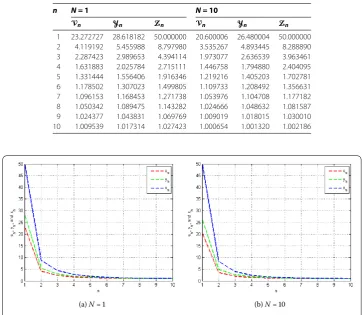
Table 1 The values of{Vn},{Yn}, and{Zn}withZ1= 50

n N= 1 N= 10

Vn Yn Zn Vn Yn Zn

1 23.272727 28.618182 50.000000 20.600006 26.480004 50.000000 2 4.119192 5.455988 8.797980 3.535267 4.893445 8.288890 3 2.287423 2.989653 4.394114 1.973077 2.636539 3.963461 4 1.631883 2.025784 2.715111 1.446758 1.794880 2.404095 5 1.331444 1.556406 1.916346 1.219216 1.405203 1.702781 6 1.178502 1.307023 1.499805 1.109733 1.208492 1.356631 7 1.096153 1.168453 1.271738 1.053976 1.104708 1.177182 8 1.050342 1.089475 1.143282 1.024666 1.048632 1.081587 9 1.024377 1.043831 1.069769 1.009019 1.018015 1.030010 10 1.009539 1.017314 1.027423 1.000654 1.001320 1.002186

(a)N=  (b)N= 

Figure 1 The convergence of{Vn},{Yn}, and{Zn}with initial valueZ1= 50.

Then we have ⎧ ⎨ ⎩

Yn=__nn_+P[,]Zn+ ( –__nn_+)_+n n+

(Zn+ __nn_+),

Zn+=__nZn+ (I–__nA)P[,](I–_n(I–T))Yn, ∀n∈N.

(.)

From Corollary ., we can conclude that the sequences{Zn},{Yn}, and{Vn}generated by (.) converge strongly to .

Table  and Figure  show the values of sequences{Zn},{Yn}, and{Vn}in two cases.

Remark .

(i) From Table  and Figure , the sequences{Zn},{Yn}, and{Vn}converge to , where

{}=Fix(T)∩N_i_=EP(i).

(ii) For case (i), Corollary . guarantees the convergence of{Zn},{Yn}, and{Vn}.

(iii) For case (ii), the convergence of{Zn},{Yn}, and{Vn}can be guaranteed by

Theorem ..

(iv) The iteration (.) for the combination of equilibrium problem converges faster than the iteration (.) for the classical equilibrium problem.

(22)

Example . LetR_{be the two-dimensional space of real numbers with an inner product} ·,·:R_×_R_→_R_{deﬁned by}_u,_v₌_u_·_v₌_u

v+uvand a usual norm · :R→R

given byu=u

+u, for allu= (u,u),v= (v,v)∈R. Let the mappingsA:R→

R_,_F _:_R_→_R_{be deﬁned by}

Au= u , u  ,

Fu= u , u 

, for allu= (u,u)∈R.

For everyi= , , . . . ,NandI= [, ], leti:I×I→RandT :I→Ibe deﬁned by

Tu=

u+ 

 , u+ 



,

i(u,v) =i(v–u)·(v+ u–), for allu= (u,u),v= (v,v)∈I,

where= (, ). Letγ = ,δn=

 n,θn=

n

n+,ϕn= n

n+, andψn= 

n for everyn∈N.

It is clear thatT is a nonspreading mapping andFix(T) ={}, where= (, ). Putai= 

i +_N_N, for everyi= , , . . . ,N. It is obvious that

N

i=aiisatisﬁes all con-ditions in Theorem . andEP(N_i_=aii) =

N

i=EP(i) ={}, where= (, ). Then we have

Fix(T)∩ N

i=

EP(i) ={}.

Then, by Theorem ., the sequencesZn= (Zn,Zn),Yn= (Yn,Yn), andVn= (Vn,Vn) con-verge strongly to{}.

Remark . From Example ., puttingρ=N_i_=(

i+_N_N)i, we obtain

≤ N

i=

aii(Vn,y) + 

ϕn

y–Vn,Vn–Zn

=ρ(y–Vn)·y+ Vn– (, )

+ 

ϕn

(y–Vn)·(Vn–Zn)

=ρy–Vn,y–Vn

·y+ Vn– ,y+ Vn– 

+ 

ϕn

y–Vn,y–Vn

·V_n–Z_n,V_n–Z_n

=ρy–Vn

y+ Vn– 

+y–Vn

y+ Vn– 

+ 

ϕn

y–Vn

V_n–Z_n+y–Vn

V_n–Z_n

=

ρy–Vn

y+ Vn– 

+ 

ϕn

y–Vn

V_n–Z_n

+

ρy–Vn

y+ Vn– 

+ 

ϕn

y–Vn

V_n–Z_n

⇔ ≤ρϕn

y–Vn

y+ Vn– 

+y–Vn

(23)

+ρϕn

y–Vn

y+ Vn– 

+y–Vn

V_n–Z_n

=ρϕn(y)+

ρV_nϕn+Vn–Zn– ρϕn

y

+ ρϕnVn–

V_n– ρϕn

V_n+V_nZ_n

+ρϕn(y)+

ρV_nϕn+Vn–Zn– ρϕn

y

+ ρϕnVn–

V_n– ρϕn

V_n+V_nZ_n

=G(y) +G(y), (.)

whereG(y) =ρϕn(y)+ (ρVnϕn+Vn–Zn– ρϕn)y+ ρϕnVn– (Vn)– ρϕn(Vn)+ V

nZnandG(y) =ρϕn(y)+(ρVnϕn+Vn–Zn–ρϕn)y+ρϕnVn–(Vn)–ρϕn(Vn)+ V

nZn. ThenG(y) andG(y) are quadratic functions with coeﬃcientsa=ρϕn,b=

ρV

nϕn+Vn–Zn– ρϕn, andc= ρϕnVn– (Vn)– ρϕn(Vn)+VnZn, anda=ρϕn,

b= ρVnϕn+Vn–Zn– ρϕn, andc= ρϕnVn– (Vn)– ρϕn(Vn)+VnZn, respectively. Determine the discriminantofGas follows:

= (b)– ac

=ρV_nϕn+Vn–Zn– ρϕn 

– ρϕn

ρϕnVn–

V_n– ρϕn

V_n+V_nZ_n

=V_n– ρϕn+ ρϕnVn–Zn 

.

From (.), ifG(y)≥,∀y∈R, it has at most one solution inR, thus≤. It follows

that

V_n=Z



n+ ρϕn  + ρϕn

. (.)

Next, we determine the discriminantofGas follows:

= (b)– ac

=ρV_nϕn+Vn–Zn– ρϕn 

– ρϕn

ρϕnVn–

V_n– ρϕn

V_n+V_nZ_n

=V_n– ρϕn+ ρϕnVn–Zn 

.

From (.), ifG(y)≥,∀y∈Rand it has at most one solution inR, then≤. This

yields

V_n=Z



n+ ρϕn  + ρϕn

. (.)

Putδn=__n,θn=__nn_+,ϕn=__nn_+,ψn=_n, for alln∈N. It is obvious that the sequences{δn},

{θn},{ϕn}, and{ψn}satisfy all conditions in Theorem .. For everyn∈N, from (.) and (.), the iterative scheme (.) becomes

⎧ ⎨ ⎩

Yn=__nn_+PCZn+ ( –__nn_+)Un,

Zn+=__nZn+ (I–__nA)PC(I–_n(I–T))Yn, ∀n∈N,

(.)

whereZn= (Zn,Zn),Yn= (Yn,Yn), andVn= (Vn,Vn) = (

Z n+ρϕn +ρϕn ,

(24)

Let the initial values be deﬁned as in the following cases.

(i) Z= (Z,Z) = (–, ),N= , andn= ,

(ii) Z= (Z,Z) = (–, )andn=N= .

For case (i), withN= , we haveρ= . Then, from (.) and (.), we obtain

V_n=Z



n+ ϕn  + ϕn

and

V_n=Z



n+ ϕn  + ϕn

.

Then we have ⎧ ⎨ ⎩

Yn=__nn_+PCZn+ ( –__nn_+)Vn,

Zn+=__nZn+ (I–__nA)PC(I–_n(I–T))Yn, ∀n∈N,

(.)

whereZn= (Zn,Zn),Yn= (Yn,Yn), andVn= (Vn,Vn) = (

Zn+ϕn +ϕn ,

Zn+ϕn +ϕn ).

Tables  and  and Figure  show the values of the sequences{Zn},{Yn}, and{Vn}in the two cases.

Table 2 The values of{Vn},{Yn}, and{Zn}withZ1= (–1, 0) andN= 1

n Vn= (Vn1,Vn2) Yn= (Yn1,Y2n) Zn= (Z1n,Z2n)

1 (0.473684, 0.736842) (0.178947, 0.589474) (–1.000000, 0.000000) 2 (0.880767, 0.899610) (0.761533, 0.799220) (0.463450, 0.548246) 3 (0.944343, 0.947678) (0.873506, 0.881086) (0.731833, 0.747902) 4 (0.967678, 0.968228) (0.920665, 0.922015) (0.838391, 0.841141) 5 (0.978604, 0.978548) (0.944718, 0.944575) (0.890502, 0.890217)

. . .

10 (0.992787, 0.992723) (0.979067, 0.978881) (0.961231, 0.960887) .

. .

. . .

16 (0.995890, 0.995878) (0.987473, 0.987437) (0.977477, 0.977412) 17 (0.996158, 0.996149) (0.988232, 0.988203) (0.978908, 0.978856) 18 (0.996393, 0.996386) (0.988903, 0.988879) (0.980164, 0.980121) 19 (0.996601, 0.996595) (0.989499, 0.989479) (0.981276, 0.981241) 20 (0.996785, 0.996780) (0.990033, 0.990017) (0.982268, 0.982239)

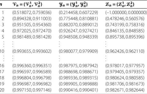
Table 3 The values of{Vn},{Yn}, and{Zn}withZ1= (–1, 0),N= 20

n Vn= (Vn1,Vn2) Yn= (Yn1,Y2n) Zn= (Z1n,Z2n)

1 (0.518072, 0.759036) (0.214458, 0.607229) (–1.000000, 0.000000) 2 (0.894328, 0.911003) (0.775448, 0.810881) (0.478246, 0.560576) 3 (0.951505, 0.954360) (0.882070, 0.889012) (0.743199, 0.758316) 4 (0.972025, 0.972470) (0.926247, 0.927421) (0.846135, 0.848585) 5 (0.981489, 0.981428) (0.948508, 0.948339) (0.895738, 0.895396)

. . .

10 (0.993655, 0.993602) (0.980077, 0.979909) (0.962426, 0.962110) .

. .

. . .

(25)

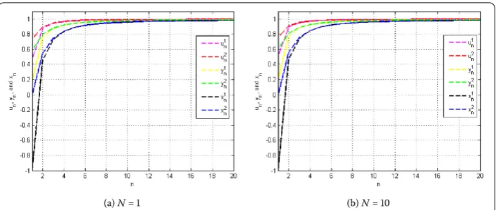
(a)N=  (b)N= 

Figure 2 The convergence of{Vn},{Yn}, and{Zn}with initial valueZ1= (–1, 0) for both cases.

Remark .

(i) Tables  and , and Figure  show that the sequences{Zn},{Yn}, and{Vn}converge

to, where{}={(, )}=Fix(T)∩N_i_=EP(i).

(ii) For case (i), Corollary . guarantees the convergence of{Zn},{Yn}, and{Vn}.

(iii) For case (ii), the convergence of{Zn},{Yn}, and{Vn}can be guaranteed by

Theorem ..

(iv) The iteration (.) for the combination of equilibrium problem converges faster than the iteration (.) for the classical equilibrium problem.

Competing interests

The authors declare that they have no competing interests.

Authors’ contributions

Both authors contributed equally and signiﬁcantly to this research article. Both authors read and approved the ﬁnal manuscript.

Acknowledgements

The authors appreciated the referees providing valuable comments improving the content of this research paper. This research is supported by the Research Administration Division of King Mongkut’s Institute of Technology Ladkrabang.

Received: 31 January 2014 Accepted: 19 July 2014 Published:15 Aug 2014

References

1. Kohsaka, F, Takahashi, W: Fixed point theorems for a class of nonlinear mappings related to maximal monotone operators in Banach spaces. Arch. Math.91, 166-177 (2008)

2. Iemoto, S, Takahashi, W: Approximating common ﬁxed points of nonexpansive mappings and nonspreading mappings in a Hilbert space. Nonlinear Anal.71, 2082-2089 (2009)

3. Kurokawa, Y, Takahashi, W: Weak and strong convergence theorems for nonspreading mappings in Hilbert spaces. Nonlinear Anal.73, 1562-1568 (2010)

4. Osilike, MO, Isiogugu, FO: Weak and strong convergence theorems for nonspreading-type mappings in Hilbert spaces. Nonlinear Anal.74, 1814-1822 (2011)

5. Liu, H, Wang, J, Feng, Q: Strong convergence theorems for maximal monotone operators with nonspreading mappings in a Hilbert space. Abstr. Appl. Anal. (2012). doi:10.1155/2012/917857

6. Deng, BC, Chen, T, Li, FL: Viscosity iteration algorithm for aρ-strictly pseudononspreading mapping in a Hilbert space. J. Inequal. Appl.2013, 80 (2013)

7. Blum, E, Oettli, W: From optimization and variational inequalities to equilibrium problems. Math. Stud.63(14), 123-145 (1994)

8. Combettes, PL, Hirstoaga, SA: Equilibrium programming in Hilbert spaces. J. Nonlinear Convex Anal.6(1), 117-136 (2005)

9. Ceng, LC, Al-Homidan, S, Ansari, QH, Yao, JC: An iterative scheme for equilibrium problems and ﬁxed point problems of strict pseudo-contraction mappings. J. Comput. Appl. Math.223, 967-974 (2009)