Meta-analysis of test accuracy studies: an exploratory method for investigating the impact of missing thresholds

(1)

M E T H O D O L O G Y

Open Access

Meta-analysis of test accuracy studies: an

exploratory method for investigating the

impact of missing thresholds

Richard D Riley

1*

, Ikhlaaq Ahmed

3

, Joie Ensor

2

, Yemisi Takwoingi

2

, Amanda Kirkham

2

, R Katie Morris

4,5

,

J Pieter Noordzij

6

and Jonathan J Deeks

2

Abstract

Background:Primary studies examining the accuracy of a continuous test evaluate its sensitivity and specificity at one or more thresholds. Meta-analysts then usually perform a separate meta-analysis for each threshold. However, the number of studies available for each threshold is often very different, as primary studies are inconsistent in the thresholds reported. Furthermore, of concern is selective reporting bias, because primary studies may be less likely to report a threshold when it gives low sensitivity and/or specificity estimates. This may lead to biased meta-analysis results. We developed an exploratory method to examine the potential impact of missing thresholds on conclusions from a test accuracy meta-analysis.

Methods:Our method identifies studies that contain missing thresholds bounded between a pair of higher and lower thresholds for which results are available. The bounded missing threshold results (two-by-two tables) are then imputed, by assuming a linear relationship between threshold value and each of logit-sensitivity and logit-specificity. The imputed results are then added to the meta-analysis, to ascertain if original conclusions are robust. The method is evaluated through simulation, and application made to 13 studies evaluating protein:creatinine ratio (PCR) for detecting proteinuria in pregnancy with 23 different thresholds, ranging from one to seven per study. Results:The simulation shows the imputation method leads to meta-analysis estimates with smaller

mean-square error. In the PCR application, it provides 50 additional results for meta-analysis and their inclusion produces lower test accuracy results than originally identified. For example, at a PCR threshold of 0.16, the summary specificity is 0.80 when using the original data, but 0.66 when also including the imputed data. At a PCR threshold of 0.25, the summary sensitivity is reduced from 0.95 to 0.85 when additionally including the imputed data.

Conclusions:The imputation method is a practical tool for researchers (often non-statisticians) to explore the potential impact of missing threshold results on their meta-analysis conclusions. Software is available to implement the method. In the PCR example, it revealed threshold results are vulnerable to the missing data, and so stimulates the need for advanced statistical models or, preferably, individual patient data from primary studies.

Keywords:Meta-analysis, Diagnostic test, Multiple thresholds, Imputation, Missing data, Sensitivity analysis

* Correspondence:[email protected] 1

Research Institute of Primary Care and Health Sciences, Keele University, Staffordshire ST5 5BG, UK

Full list of author information is available at the end of the article

(2)

Background

Medical tests are used to inform screening, diagnosis and prognosis in medicine. Meta-analysis methods are increasingly used to synthesise the evidence about a test’s accuracy from multiple studies, to produce sum-mary estimates of sensitivity and specificity [1-4]. When the test is measured on a continuous scale, many studies report test performance at multiple thresholds, each re-lating to a different choice of threshold above which test results are classed as‘positive’and below which test re-sults are classed as ‘negative’. Unfortunately, most pri-mary studies do not report the same set of thresholds. For example, in an evaluation of the spot protein:cre-atinine ratio (PCR) for detecting significant proteinuria in pregnancy, Morris et al. [5] extracted tables for 23 different thresholds across 13 studies; eight of the thresholds were considered by just one study, but the other 15 thresholds were considered in two or more studies (Table 1), with a maximum of six studies for any threshold. In this situation, meta-analysts generally either utilise the results for just one of the thresholds per study or utilise results for all reported thresholds but perform a separate meta-analysis for each of the thresholds independently [6]. However, an approach that considers meta-analysis for each threshold inde-pendently will omit any studies that do not report the threshold of interest and thus also ignore information from other thresholds that are available in those studies.

In this article, we propose an exploratory method (a sensitivity analysis) to help researchers examine the po-tential impact of missing thresholds on their meta-analysis conclusions about a test’s accuracy. The method first imputes results in studies where missing thresholds are bounded between a pair of known thresholds; missing results are also bounded because as the threshold value increases, sensitivity must decrease and specificity must increase. The imputed results are then added to the meta-analysis, and this allows re-searchers to evaluate whether their original conclusions are robust. This is especially important when thresholds are prone to selective reporting bias; that is, they are less likely to be reported when they give lower values of sensitivity and/or specificity. In this situation, meta-analysis may otherwise produce summary sensitivity and specificity results that are too high (i.e. biased).

The article is structured as follows. In the“Motivating example”section, we describe the motivating PCR data-set in detail. In the“Methods”section, we describe our imputation method, explain its assumptions and per-form an empirical evaluation. The “Results”section ap-plies it to the PCR data, and the “Discussion” section concludes by considering the strengths and limitations of the method and further research.

Motivating example: identification of significant proteinuria in patients with suspected pre-eclampsia

Pre-eclampsia is a major cause of maternal and perinatal morbidity and mortality and occurs in 2%–8% of all pregnancies [7-10]. The diagnosis of pre-eclampsia is de-termined by the presence of elevated blood pressure combined with significant proteinuria (≥0.3 g per 24 h) after the 20th week of gestation in a previously normoten-sive, non-proteinuric patient [11]. The gold-standard method for detection of significant proteinuria is the 24-h urine collection, but this is cumbersome, time consuming and inconvenient, to patients as well as hospital staff. There is therefore a need for a rapid and accurate diagnos-tic test to identify significant proteinuria to allow more timely decision-making.

The spot PCR has been shown to be strongly corre-lated with 24-h protein excretion and thus is a potential diagnostic test for significant proteinuria. Morris et al. [5] performed a systematic review and meta-analysis to assess the diagnostic accuracy of PCR for the detection of significant proteinuria in patients with suspected pre-eclampsia. Thirteen relevant studies were identified, and in each study, the reference standard was proteinuria greater than or equal to 300 mg in urine over 24 h. Across the 13 studies, 23 different threshold values were considered for PCR, ranging from 0.13 to 0.50. Five studies provided diagnostic accuracy results (i.e. a two-by-two table showing the number of true posi-tives, false posiposi-tives, false negatives and true negatives) for just one threshold, but the other eight studies re-ported results for each of multiple thresholds, up to a maximum of nine thresholds (Yamasmit study). Eight of the 23 thresholds were considered by just one study, but the other 15 thresholds were considered in two or more studies, up to a maximum of six studies (for threshold 0.20). The studies and thresholds are sum-marised in Table 1.

Meta-analysis is important here to summarise the diagnostic accuracy of PCR at each threshold from all the published evidence, to help ascertain whether PCR is a useful diagnostic test and, if so, which threshold is the most appropriate to use in clinical practice. However, this is non-trivial given the number of thresholds avail-able, the variation in how many studies report each threshold and the likely similarity between neighbouring threshold results. The PCR data is thus an ideal dataset to motivate and apply the statistical methods developed during the remainder of the paper.

Methods

(3)

Table 1 PCR results for each threshold in each of the 13 studies of Morris et al. [5]

First author Threshold ID,t Threshold value,x TP FP FN TN Total High proteinuria Normal proteinuria

Al Ragib 1 0.13 35 51 4 95 185 39 146

6 0.18 33 42 6 104

7 0.19 33 39 6 107

8 0.2 31 38 8 108

22 0.49 29 23 10 123

Durnwald 3 0.15 156 35 12 17 220 168 52

8 0.2 152 27 16 25

15 0.3 136 23 32 29

19 0.39 123 14 45 38

20 0.4 120 12 48 40

23 0.5 106 9 62 43

Dwyer 3 0.15 54 28 2 32 116 56 60

5 0.17 51 25 5 35

7 0.19 50 18 6 42

12 0.24 41 8 15 52

14 0.28 37 3 19 57

19 0.39 31 0 25 60

Leonas 15 0.3 277 7 5 638 927 282 645

Ramos 23 0.5 25 1 1 20 47 26 21

Robert 15 0.3 27 4 2 38 71 29 42

Rodriguez 2 0.14 69 34 0 35 138 69 69

3 0.15 68 34 1 35

4 0.16 68 26 1 43

5 0.17 65 25 4 44

6 0.18 62 24 7 45

7 0.19 62 21 7 48

8 0.2 60 19 9 50

9 0.21 60 17 9 52

Saudan 8 0.2 14 27 0 59 100 14 86

13 0.25 13 14 1 72

15 0.3 13 7 1 79

18 0.35 12 4 2 82

20 0.4 11 3 3 83

21 0.45 10 0 4 86

Schubert 3 0.15 9 3 0 3 15 9 6

4 0.16 9 2 0 4

Shahbazian 8 0.2 35 2 3 41 81 38 43

Taherian 2 0.14 67 7 6 20 100 73 27

3 0.15 67 3 6 24

4 0.16 65 1 8 26

5 0.17 64 1 9 26

6 0.18 63 0 10 27

8 0.2 59 0 14 27

(4)

Exploratory method to examine the potential impact of missing thresholds

Let there bei= 1 tomstudies that measure a continu-ous test result on n1i diseased patients and n0i

non-diseased patients, whose true disease status is pro-vided by a reference standard. In each study, at a par-ticular threshold value, x, each patient’s measured test value is classed as either ‘positive’ (≥x) or ‘negative’ (<x). Then summarising test results over all patients produces aggregate data in the form ofr11ix, the

num-ber of truly diseased patients in studyiwith a positive test result at threshold x, and r00ix, the number of

non-diseased patients in study i with a negative test result. The observed sensitivity at threshold x in each study is thus simplyr11ix/n1i and the observed

specifi-city isr00ix/n0i.

When results for a particular threshold are missing but other thresholds above and below are available, then the missing threshold has sensitivity and specificity re-sults constrained between these values. For example, consider the Al Ragib study (Table 1), which has thresh-old values of 0.13 and 0.18 available, but not 0.14 to 0.17. The number of true positives for the missing thresholds must be constrained between the other threshold values of 35 and 33. Similarly, the missing false positives must be within 42 and 51, the missing false negatives within 4 and 6 and the missing true nega-tives within 95 and 104.

Rather than ignoring missing thresholds that are bounded between known thresholds, our exploratory method imputes the missing results under particular assumptions, so that they can be included in the meta-analysis. The aim is to ascertain whether the original meta-analysis conclusions (obtained without imputed data) are robust to the inclusion of imputed data. For example, does the summary test accuracy at each threshold remain similar, and is the choice of best threshold the same? The exploratory method is a two-step approach, as now described.

Step 1: imputation of missing bounded thresholds in each study

In each study separately, for each threshold that is miss-ing but bounded between known thresholds, the missmiss-ing results are imputed by assuming each 1-unit increase in threshold value corresponds to a constant reduction in logit-sensitivity (y1ix), and also a constant increase in

logit-specificity (y0ix). Thus, imputation is on a straight

line between pairs of observed points in logit receiver operating characteristic (ROC) space. This piece-wise linear approach is illustrated graphically in Figure 1. So the key assumption here is a constant change in logit values for each 1-unit change in threshold value between each pair of observed threshold results. The linear slope can be different between each pair of thresholds, and so no single trend is assumed across all thresholds, with the fitted lines forced to go through the observed points. Linear relationships on the logit scale are often used in diagnostic test analyses when considering the ROC curve, especially in meta-analysis [12], and it is a straightforward approach for this exploratory analysis.

Once the imputed logit values are obtained, one can back transform to compute the corresponding imputed true and false positives and negatives. For example, let TP1 be the true positive number at a threshold value of 0.13 and TP2 be the true positive number at threshold 0.18. Then, in the Al Ragib study there are 5 threshold units from 0.13 to 0.18. The imputed logit-sensitivity at threshold 0.14 is y1i(0.13)+ (y1i(0.18)−y1i(0.13))/5, and at threshold 0.15 the imputed logit-sensitivity is y1i(0.13)+ (2(y1i(0.18)−y1i(0.13))/5), and so on (Table 2, Figure 1). It is then straightforward to calculate the number of true positives, false positives, true negatives and false nega-tives that are necessary to produce these values. For ex-ample, for threshold 0.15, the imputed logit-sensitivity is 1.983, and so the imputed sensitivity is 0.879, and given there are 39 patients truly with high proteinuria, the im-puted number of true positives and false negatives is 34.28 and 4.72, respectively (Table 2).

Table 1 PCR results for each threshold in each of the 13 studies of Morris et al. [5](Continued)

Yamasmit 7 0.19 29 6 0 7 42 29 13

9 0.21 29 5 0 8

10 0.22 29 4 0 9

11 0.23 28 3 1 10

12 0.24 28 2 1 11

13 0.25 28 1 1 12

14 0.28 27 1 2 12

16 0.31 26 1 3 12

17 0.32 25 1 4 12

(5)

Note that we neither impute beyond the highest available threshold nor impute below the lowest avail-able threshold in each study. Further assumptions would be necessary to do this, but here we only work within the limits of the observed data available. Thus, for studies with only 1 threshold reported, no imput-ation was used. Similarly, we do not impute for any new threshold values which were not considered by any of the available studies.

A STATA ‘do’ file to fit the imputation method is available in Additional file 1, and we aim to release an associated STATA module in the near future. It pro-vides the original and imputed values within a few seconds, for any number of studies and any number of thresholds.

Step 2: meta-analysis at each threshold separately using actual and imputed data

The imputation in step 1 borrows strength from avail-able thresholds to allow a larger set of threshold data to be available from each study for meta-analysis. For ease of language, let us order the thresholds of interest and refer to the ordered value as t (e.g. t= 1 to 23 in the PCR example, Table 1). Each threshold t now has (i) one or more studies with observed results and poten-tially (ii) some studies with imputed results. A separate meta-analysis of each threshold separately can now be considered, using the observed and imputed results. A convenient model is the bivariate meta-analysis of Chu and Cole [2]. This approach is recommended by the Cochrane Screening and Diagnostic Test Methods

.17

.32

.23

.39

.3

.14

.28 .31

.24

.4

.22.21

.16

.25

.35

.15

.45

.19 .18

.2

.49

.13

1

1.25

1.5

1.75

2

2.25

logit−sensitivity

.5 .75

1 1.25

1.5 1.75

logit−specificity

imputed observed

Figure 1Graphical illustration of the imputation approach for the Al Ragib study.

Table 2 Actual and imputed results for the Al Ragib study between thresholds 0.13 and 0.18

First author Threshold ID,t Threshold value,x Imputed? TP FP FN TN Total High proteinuria Normal proteinuria

Al Ragib 1 0.13 No 35 51 4 95 185 39 146

2 0.14 Yes 34.7 49.1 4.3 96.9

3 0.15 Yes 34.3 47.3 4.7 98.7

4 0.16 Yes 33.9 45.5 5.1 100.5

5 0.17 Yes 33.5 43.7 5.5 102.3

6 0.18 No 33 42 6 104

The imputation is undertaken on the logit-scale, and then the values are back transformed to calculate the corresponding imputed raw data values.

(6)

Group and is commonly used in diagnostic accuracy meta-analyses. It utilises the exact binomial within-study distribution, thereby avoiding the need for any continuity corrections, and accounts for any between-study correl-ation in sensitivity and specificity, as follows:

TP_it_eBinomial n1i;sensitivityit

logit sensitivity _it¼β1tþu1t

TNiteBinomial n0 i; specificity_it

logit specificity _it¼β₀_tþu0t u1t

u0t

eN 00 ;Ωt

; Ωt¼ τ

2

1t τ1tτ0tρ10t

τ1tτ0tρ10t τ20t

ð1Þ

β1t and β0tgive the average logit-sensitivity and

aver-age logit-specificity at thresholdt, respectively, and these can be transformed to give the summary sensitivity and summary specificity from the meta-analysis for each threshold. The between-study covariance matrix is given byΩ_t, containing the between-study variances (τ2

1tandτ20t)

and the between-study correlation in logit-sensitivity and logit-specificity (ρ10t); if the latter is zero, the model re-duces to a separate univariate analysis for each of sensitiv-ity and specificsensitiv-ity. Indeed, ρ10t will often be poorly estimated at +1 or−1 [13], and so it may be sensible to adopt two separate univariate models here [14], as follows:

TPit_eBinomial n 1i;sensitivity_it logit sensitivity _it¼β_1tþu_1t

TN_it_eBinomial n 0i;specificity_it logit specificity _it¼β_0tþu0t

u1t

u0t

eN 00 ;Ωt

; Ωt¼ τ 2 1t 0

0 τ2

0t

ð2Þ

Models (1) and (2) can be estimated using adaptive Gaussian quadrature [15], for example using PROC NLMIXED in SAS [16], or the xtmelogit command in STATA [17]. A number of quadrature points can be spe-cified, with increasing estimation accuracy as the num-ber of points increases, but at the expense of increased computational time. We generally chose 5 quadrature points for our analyses, as this gave estimates very close to those when using >10 points but in a faster time. Successful convergence of the optimization procedure was assumed when successive iteration estimates differed by <10−7, resulting in parameter estimates and their approximate standard errors based on the second derivative matrix of the likelihood function.

Empirical evaluation of the imputation method

To empirically evaluate the imputation method, we uti-lised individual participant data (IPD) from six studies examining the ability of parathyroid hormone (PTH) to correctly classify which patients will become hypocalcemic within 24-h after a thyroidectomy [18]. The percentage

decrease in PTH (from pre-surgery to 6-h post-surgery) was used as the test, and thresholds of 40%, 50%, 60%, 65%, 70%, 80% and 90% were examined. As IPD were available, the results for all thresholds were available for all studies. Thus, for each threshold separ-ately, we could fit model (1) using the complete set of data from the six studies. However, model (1) often poorly estimated the between-study correlations at +1 or −1 and gave summary test accuracy results very similar to model (2). Thus we focus here only on model (2) results, and these provided our ‘complete data’ meta-analysis results, for when the thresholds are all truly available from all studies.

Generation of missing thresholds and imputation

To replicate missing data mechanisms, we considered two scenarios:

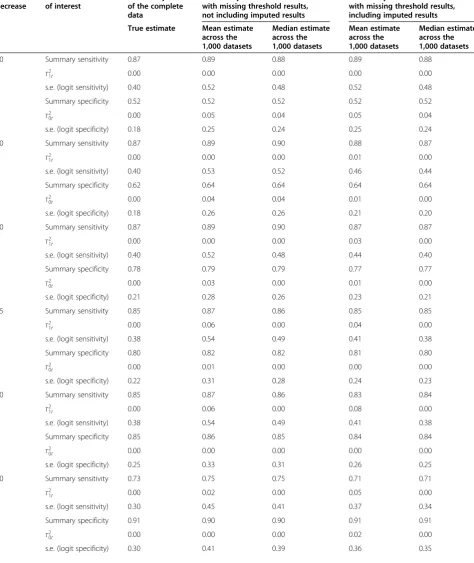
Scenario (i): thresholds missing at random We took the complete set of threshold results for each study and randomly assigned some to be missing, with each hav-ing a 0.5 probability of behav-ing omitted. This provided a new meta-analysis dataset of up to six studies with missing threshold results. We repeated this process until 1,000 such meta-analysis datasets had been pro-duced. In each dataset, we applied our imputation ap-proach, and then for each threshold, we fitted model (2) to (i) each generated dataset without including the imputed results and (ii) each generated dataset with the addition of the imputed results. We then compared the average meta-analysis estimates and standard errors from the 1,000 analyses of (i) and (ii) with the true meta-analysis results when the complete data were available (Table 3).

(7)

Table 3 Empirical evaluation results—scenario (i), thresholds missing at random

% PTH decrease

Estimate of interest

Meta-analysis of the complete data

Meta-analysis of the datasets with missing threshold results, not including imputed results

Meta-analysis of the datasets with missing threshold results, including imputed results

True estimate Mean estimate across the 1,000 datasets

Median estimate across the 1,000 datasets

Mean estimate across the 1,000 datasets

40 Summary Sensitivity 0.87 0.88 0.90 0.88 0.90

τ2

1t 0.00 0.04 0.00 0.04 0.00

s.e. (logit sensitivity) 0.40 0.70 0.62 0.70 0.62

Summary specificity 0.52 0.52 0.52 0.52 0.52

τ2

0t 0.00 0.05 0.00 0.05 0.00

s.e. (logit specificity) 0.18 0.25 0.24 0.25 0.24

50 Summary sensitivity 0.87 0.88 0.90 0.87 0.87

τ2

1t 0.00 0.04 0.00 0.04 0.00

τ2

0t 0.00 0.05 0.01 0.04 0.00

τ2

1t 0.00 0.04 0.00 0.05 0.00

τ2

0t 0.00 0.05 0.00 0.05 0.00

τ2

1t 0.00 0.04 0.00 0.05 0.00

τ2

0t 0.00 0.05 0.00 0.04 0.00

τ2

1t 0.00 0.07 0.00 0.05 0.00

τ2

0t 0.00 0.04 0.00 0.04 0.00

τ2

1t 0.00 0.04 0.00 0.05 0.00

τ2

0t 0.00 0.04 0.00 0.04 0.00

(8)

Results

Results of empirical evaluation

In the empirical evaluation, there is no imputation for the lowest and highest threshold of 40% and 90%, and so meta-analysis results are identical for these thresholds regardless of whether imputed data is included or not. However, for other thresholds, there is always potential for imputation.

For thresholds between 40% and 90% in scenario (i), where thresholds were missing at random, the mean and median estimates tend to be slightly closer to the complete data results when using the imputed data (Table 3). For example, at threshold 65%, the true sensi-tivity estimate from complete data is 0.85, whilst the mean/median without using imputed data is 0.87/0.89, but when using the imputed data, it is pulled back to 0.85/0.85. Further, the meta-analyses including the im-puted data give substantially smaller standard errors than those from the meta-analyses excluding imputed data. For example, for threshold 65%, the standard error of the summary logit-sensitivity is 0.69 when ignoring imputed data and 0.49 when including it, a gain in preci-sion of almost 30%. The gain in standard error reflects the additional information being used from the imputed results. As estimates are close to the true estimates and standard errors are considerably reduced, the mean-square error of estimates is therefore improved. The im-putation approach also gives standard errors of estimates that are also closer (but not smaller) to those from the true complete data meta-analysis.

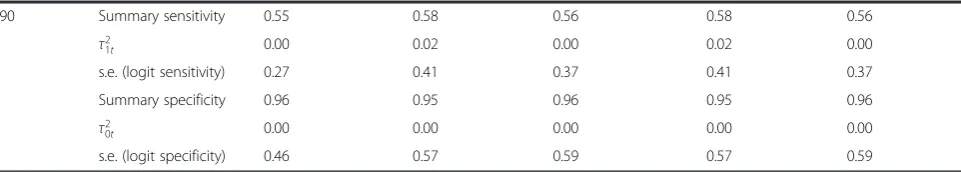
For scenario (ii), where thresholds are selectively miss-ing based on the value of observed sensitivity, the sum-mary meta-analysis results without the imputed data are again slightly larger than the true estimated values, espe-cially for sensitivity. The meta-analysis results using the imputed data generally reduce this bias and give more conservative estimates. For example, for the 50% thresh-old, the true estimated value for sensitivity is 0.87, whilst the median meta-analysis estimate without imputation data is 0.90, but the median estimate including imputed data is pulled back down to 0.87. Occasionally, the im-putation method over-adjusted, so that the estimate was pulled down too far. For example, for the 80% threshold,

the true estimated value for sensitivity is 0.73, but the median estimate from the without imputation data is 0.75 and the median estimate from the imputed data is 0.71. However, even here the absolute magnitude of bias is the same (0.02) with and without imputed data. For all thresholds between 40% and 90%, there is again consid-erable reduction in the standard error of meta-analysis estimates following the use of imputed data.

In summary, the empirical evaluation shows that the imputation method performs well, with summary test accuracy estimates generally moved slightly closer to the true estimates based on complete data. This finding, combined with smaller standard errors and thus smaller mean-square error of estimates, suggests the imputation approach is useful as an exploratory analysis.

Application to the PCR example

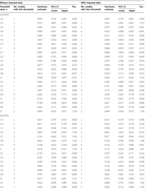
Our imputation approach was applied to the PCR stud-ies introduced in the“Motivating example” section, and missing threshold results could be imputed in 6 of the 13 studies. For 21 of the 23 different thresholds, the im-putation approach increased the number of studies pro-viding data for that threshold (Table 5), and in total, an additional 50 thresholds results were imputed, substan-tially increasing the information available for meta-analysis. For example, at a PCR threshold of 0.22, the imputation increased the available studies from 1 to 5, and at a threshold of 0.3, the available studies increased from 4 to 7.

Meta-analysis model (1) was applied to each thresh-old’s data separately, but the between-study correlations were often estimated poorly as −1 in these analyses, so we decided to rather fit model (2) (i.e. ρ10t was set to zero for all analyses, allowing a separate analysis for sen-sitivity and specificity at each threshold) [14]. The sum-mary meta-analysis results when including or ignoring the imputed data are shown for each threshold in Table 5 and Figure 2.

Importantly, the results when including the imputed data are often very different to when ignoring it. In par-ticular, the summary estimates of sensitivity and specifi-city are generally reduced when using the imputed data, as can be seen visually in the summary ROC space

Table 3 Empirical evaluation results—scenario (i), thresholds missing at random(Continued)

τ2

1t 0.00 0.05 0.00 0.05 0.00

τ2

0t 0.00 0.04 0.00 0.04 0.00

(9)

Table 4 Empirical evaluation results—scenario (ii), thresholds selectively missing

% PTH decrease

Estimate of interest

Meta-analysis of the complete data

Meta-analysis of the datasets with missing threshold results, not including imputed results

Meta-analysis of the datasets with missing threshold results, including imputed results

True estimate Mean estimate across the 1,000 datasets

Mean estimate across the 1,000 datasets

τ2

1t 0.00 0.00 0.00 0.00 0.00

τ2

0t 0.00 0.05 0.04 0.05 0.04

τ2

1t 0.00 0.00 0.00 0.01 0.00

τ2

0t 0.00 0.04 0.04 0.01 0.00

τ2

1t 0.00 0.00 0.00 0.03 0.00

τ2

0t 0.00 0.03 0.00 0.01 0.00

τ2

1t 0.00 0.06 0.00 0.04 0.00

τ2

0t 0.00 0.01 0.00 0.00 0.00

τ2

1t 0.00 0.06 0.00 0.08 0.00

τ2

0t 0.00 0.00 0.00 0.00 0.00

τ2

1t 0.00 0.02 0.00 0.05 0.00

τ2

0t 0.00 0.00 0.00 0.02 0.00

(10)

(Figure 2). For example, when imputed data were in-cluded, the summary specificity at a PCR threshold of 0.16 reduced from 0.80 to 0.66 and the summary sensi-tivity at a PCR threshold of 0.25 reduced from 0.95 to 0.85.

The points in ROC space tend to move down and to the right after including imputed data, revealing lower sensitivity and specificity than previously thought. Thus, it appears that the results when ignoring imputed data may be optimistic, potentially due to biased availability of thresholds when they give higher test accuracy results. In both analyses (assuming sensitivity and specificity are equally important), the best threshold appears to be be-tween 0.25 and 0.30; however, test accuracy at these thresholds is lower after imputation.

The dramatic change in results for some thresholds suggests that individual patient data are needed to ob-tain a complete set of threshold results from each study and thereby remove the suspected reporting bias in pri-mary studies. We also attempted to use the advanced statistical modelling framework of Hamza et al. [12] to reduce the impact of missing thresholds by jointly syn-thesising all thresholds in one multivariate model; how-ever, this approach failed to converge, most likely due to the amount of missing data. The multiple thresholds model of Putter et al. [19] also required complete data for all thresholds, whilst the method of Dukic and Gatsonis [20] was not considered suitable, as it produces a sum-mary ROC curve but does not give meta-analysis results for each threshold.

Discussion

Primary study authors often do not use the same thresh-olds when evaluating a medical test and will predomin-ately report those thresholds that produce the largest (optimal) sensitivity and specificity estimates [21]. This may lead to optimistic and misleading meta-analysis re-sults based only on reported thresholds. We have pro-posed an exploratory method for examining the impact of missing threshold results in meta-analysis of test accuracy studies and shown its potential usefulness through an ap-plied example and empirical evaluation. The imputation method is applicable when studies use the same (or

similarly validated or standardised) methods of measuring a continuous test (e.g. blood pressure or a continuous bio-marker, like prostate-specific antigen). It is deliberately very simple, so that applied researchers can still imple-ment standard meta-analysis methods and examine the potential impact of missing thresholds on meta-analysis conclusions. For example, our application to the PCR data showed how the imputation method revealed lower diag-nostic test accuracy results than a standard meta-analysis of each threshold independently, but conclusions about the best choice of threshold appeared robust.

Other more sophisticated methods are also available to deal with multiple thresholds, but all have limitations. Hamza et al. [12] propose a multivariate random-effect meta-analysis approach and apply it whenallstudies re-portall of the thresholds of interest. It models the (lin-ear) relationship between threshold value and test accuracy within each study but is prone to convergence problems (as we experienced for the PCR example), prompting Putter et al. [19] to propose an alternative survival model framework for meta-analysing the mul-tiple thresholds. However, this also requires the mulmul-tiple thresholds to be available in all studies. Others have also considered the multiple threshold issue [20,22-27]. A well-known method by Dukic and Gatsonis [20] only pro-duces a summary ROC curve, rather than summary re-sults for each threshold of interest. We recently proposed a multivariate-normal approximation to the Hamza et al. approach [27], which produces both a summary ROC curve and summary results for each threshold and easily accommodates studies with missing thresholds. However, the multivariate-normal approximation to the exact multi-nomial likelihood is a potential limitation.

Our exploratory method is not a competitor to these more sophisticated methods. Rather, it is an exploratory tool aimed at researchers (usually non-statisticians) con-ducting systematic reviews of test accuracy studies. The method is practical and easy to implement without ad-vanced statistical expertise and so can quickly flag whether researchers should be concerned about missing thresholds in their meta-analysis. This was demonstrated in the PCR example, where the method flagged major con-cerns that original conclusions were optimistic. In this

Table 4 Empirical evaluation results—scenario (ii), thresholds selectively missing(Continued)

τ2

1t 0.00 0.02 0.00 0.02 0.00

τ2

0t 0.00 0.00 0.00 0.00 0.00

(11)

Table 5 Summary meta-analysis results following application of model (2) with and without the imputed data included

Without imputed data With imputed data

Threshold value,x

No. studies with this threshold

Summary estimate

95% CI Tau No. studies with this threshold

Summary estimate

95% CI Tau

Lower Upper Lower Upper

Sensitivity

0.13 1 0.897 0.756 0.961 0.000 1 0.897 0.756 0.961 0.000

0.14 2 0.910 0.841 0.951 0.000 3 0.955 0.801 0.991 1.147

0.15 5 0.944 0.901 0.969 0.067 6 0.937 0.909 0.957 0.001

0.16 3 0.960 0.831 0.991 0.850 6 0.925 0.890 0.950 0.091

0.17 3 0.909 0.860 0.942 0.000 5 0.911 0.879 0.935 0.000

0.18 3 0.873 0.816 0.914 0.000 5 0.894 0.860 0.920 0.000

0.19 4 0.902 0.851 0.936 0.000 6 0.889 0.855 0.917 0.096

0.2 6 0.875 0.828 0.910 0.234 8 0.886 0.839 0.921 0.312

0.21 3 0.892 0.834 0.931 0.000 7 0.882 0.848 0.909 0.000

0.22 1 0.983 0.782 0.999 0.000 5 0.899 0.761 0.961 0.669

0.23 1 0.950 0.786 0.990 0.000 5 0.870 0.766 0.932 0.534

0.24 2 0.877 0.575 0.974 0.973 5 0.850 0.756 0.912 0.473

0.25 2 0.953 0.832 0.988 0.000 5 0.850 0.759 0.910 0.442

0.28 2 0.818 0.531 0.947 0.837 5 0.818 0.715 0.890 0.473

0.3 4 0.938 0.829 0.979 0.975 7 0.893 0.773 0.954 1.076

0.31 1 0.883 0.713 0.959 0.000 5 0.780 0.689 0.851 0.362

0.32 1 0.850 0.675 0.939 0.000 5 0.781 0.687 0.853 0.363

0.35 1 0.833 0.562 0.951 0.000 4 0.733 0.641 0.809 0.296

0.39 2 0.662 0.530 0.772 0.320 4 0.699 0.607 0.778 0.278

0.4 2 0.720 0.650 0.780 0.000 3 0.724 0.661 0.779 0.000

0.45 1 0.700 0.436 0.876 0.000 3 0.691 0.627 0.748 0.000

0.49 1 0.842 0.774 0.893 0.000 2 0.657 0.590 0.718 0.000

0.5 2 0.844 0.433 0.975 1.230 2 0.844 0.433 0.975 1.230

Specificity

0.13 1 0.651 0.570 0.724 0.000 1 0.651 0.570 0.724 0.000

0.14 2 0.671 0.597 0.736 0.000 3 0.624 0.524 0.714 0.250

0.15 5 0.562 0.366 0.740 0.795 6 0.583 0.421 0.728 0.717

0.16 3 0.803 0.499 0.943 1.026 6 0.661 0.462 0.816 0.910

0.17 3 0.765 0.463 0.925 1.042 5 0.677 0.465 0.834 0.922

0.18 3 0.856 0.436 0.979 1.503 5 0.726 0.458 0.893 1.188

0.19 4 0.708 0.653 0.758 0.000 6 0.720 0.522 0.858 0.961

0.2 6 0.818 0.597 0.931 1.245 8 0.775 0.609 0.884 1.031

0.21 3 0.750 0.672 0.815 0.000 7 0.707 0.635 0.771 0.332

0.22 1 0.692 0.409 0.880 0.000 5 0.705 0.599 0.793 0.438

0.23 1 0.769 0.478 0.924 0.000 5 0.738 0.623 0.828 0.508

0.24 2 0.863 0.764 0.925 0.000 5 0.762 0.636 0.855 0.592

0.25 2 0.848 0.764 0.907 0.000 5 0.798 0.655 0.892 0.724

0.28 2 0.945 0.863 0.979 0.000 5 0.845 0.681 0.933 0.947

0.3 4 0.917 0.703 0.981 1.515 7 0.916 0.793 0.969 1.311

0.31 1 0.923 0.609 0.989 0.000 5 0.886 0.707 0.962 1.183

(12)

situation, researchers should be stimulated to put

re-sources toward undertaking the aforementioned

advanced statistical methods or, ideally, obtaining indi-vidual participant data to calculate missing threshold results directly.

The key reason that we label our method as‘ explora-tory’is that it only considers single imputation. Single imputation of missing values usually causes standard errors of estimates to be too small, since it fails to ac-count for the uncertainty in the imputed values them-selves, and multiple imputations would help address this [28]. In particular, imputed data between two thresholds close together (e.g. imputing data for a threshold of 0.24 using available thresholds 0.23 and 0.25) should have less uncertainty than imputing data between two thresholds far apart (e.g. imputing at a threshold of 0.24 using thresholds 0.13 and 0.50), but this is not currently accounted for in our approach. Further research may consider extension to multiple imputations. Also, our imputation assumes a linear re-lationship between threshold value and logit-sensitivity and logit-specificity; although this linear relationship is

commonly used in meta-analysis of test accuracy stud-ies, it is of course an assumption.

Thus, our imputation method is a sensitivity analysis: it shows, under the assumptions made, how vulnerable the original meta-analysis conclusions are to the missing threshold results. The focus is therefore on how the method modifies the original summary meta-analysis es-timates; less attention should be paid to the standard er-rors and confidence intervals it produces, as these may be artificially small and narrow. The method is thus similar in spirit to how others have evaluated the poten-tial impact of (biased) missing data in meta-analysis of randomised trials, such as trim and fill [29] and adjust-ments based on funnel plot asymmetry [30]. For ex-ample, trim and fill imputes missing studies assuming asymmetry is caused by publication bias and Peters et al. [31] conclude it ‘can help to reduce the bias in pooled estimates, even though the performance of this method is not ideal … we recommend use of the trim and fill method as a form of sensitivity analysis.’ Similarly, our method can help to reduce bias and mean-square error in pooled meta-analysis results.

Conclusion

We have proposed an exploratory analysis that allows researchers to examine the potential impact of missing thresholds on the conclusions of a test accuracy meta-analysis. Currently, most researchers ignore this issue, but our PCR example shows that this may be naive, as conclusions are susceptible to selective threshold report-ing in primary studies. STATA code to fit the imputation approach is available in the Additional file 1, and an as-sociated STATA module will be released in the near future.

Additional file

Additional file 1:A STATA‘do’file to fit the proposed imputation method.

Competing interests

The authors declare that they have no competing interest.

Table 5 Summary meta-analysis results following application of model (2) with and without the imputed data included (Continued)

0.35 1 0.948 0.876 0.979 0.000 4 0.898 0.701 0.971 1.239

0.39 2 0.980 0.092 1.000 3.125 4 0.933 0.713 0.987 1.556

0.4 2 0.903 0.675 0.977 0.982 3 0.872 0.715 0.949 0.796

0.45 1 0.994 0.915 1.000 0.000 3 0.944 0.587 0.995 1.883

0.49 1 0.842 0.774 0.893 0.000 2 0.838 0.779 0.883 0.000

0.5 2 0.863 0.764 0.925 0.000 2 0.863 0.764 0.925 0.000

NB All meta-analyses used model (2), as model (1) often poorly estimatedρ10tat +1 or−1.

(13)

Authors’contributions

RR developed the method with YT and JD. IA undertook the simulation study, under supervision from RR and JD, and input from JE. JE developed the STATA code to implement the method. AK tested the feasibility of the method of a number of datasets. RKM and JPN collected the data used in the simulation and examples and provided clinical feedback on the results. RR wrote the first draft of the paper, and all authors contributed to subsequent revisions. All authors read and approved the final manuscript.

Acknowledgements

RDR, JE and JJD were supported by funding from an MRC Methodology Research Grant in Multivariate Meta-analysis (grant reference number: MR/ J013595/1). RDR was also supported by funding from NICE. RKM is funded by an NIHR Clinical Lectureship. IA was funded by the MRC Midlands Hub for Trials Methodology Research at the University of Birmingham (Medical Research Council Grant ID G0800808). We thank the reviewers for helpful feedback.

Author details 1

Research Institute of Primary Care and Health Sciences, Keele University, Staffordshire ST5 5BG, UK.2_{School of Health and Population Sciences, Public}

Health Building, University of Birmingham, Edgbaston, Birmingham B15 2TT, UK.3_{MRC Hub for Trials Methodology Research, School of Health and}

Population Sciences, Public Health Building, University of Birmingham, Edgbaston, Birmingham B15 2TT, UK.4_{Research Section of Reproduction,}

Genes and Development; School of Clinical and Experimental Medicine, College of Medical and Dental Sciences, University of Birmingham, Birmingham, UK.5Fetal Medicine Centre, Birmingham Women’s Hospital NHS Foundation Trust, Birmingham, UK.6_{Department of Otolaryngology - Head &}

Neck Surgery, Boston Medical Center, Boston University - School of Medicine, Boston, MA, USA.

Received: 25 September 2014 Accepted: 30 December 2014 Published: 4 February 2015

References

1. Reitsma JB, Glas AS, Rutjes AW, Scholten RJ, Bossuyt PM, Zwinderman AH. Bivariate analysis of sensitivity and specificity produces informative summary measures in diagnostic reviews. J Clin Epidemiol. 2005;58(10):982–90. 2. Chu H, Cole SR. Bivariate meta-analysis of sensitivity and specificity with

sparse data: a generalized linear mixed model approach. J Clin Epidemiol. 2006;59(12):1331–2. author reply 1332–1333.

3. Rutter CM, Gatsonis CA. A hierarchical regression approach to meta-analysis of diagnostic test accuracy evaluations. Stat Med. 2001;20(19):2865–84. 4. Harbord RM, Deeks JJ, Egger M, Whiting P, Sterne JA. A unification of

models for meta-analysis of diagnostic accuracy studies. Biostatistics. 2007;8(2):239–51.

5. Morris RK, Riley RD, Doug M, Deeks JJ, Kilby MD. Diagnostic accuracy of spot urinary protein and albumin to creatinine ratios for detection of significant proteinuria or adverse pregnancy outcome in patients with suspected pre-eclampsia: systematic review and meta-analysis. BMJ. 2012;345:e4342.

6. Hewitt C, Gilbody S, Brealey S, Paulden M, Palmer S, Mann R, et al. Methods to identify postnatal depression in primary care: an integrated evidence synthesis and value of information analysis. Health Technol Assess. 2009;13(36):1–145. 147–230.

7. CEMACH. Saving Mothers’Lives: reviewing maternal deaths to make motherhood safer—2003–2005. The Seventh Report on Confidential Enquiries into Maternal Deaths in the United Kingdom, The Confidential Enquiry into Maternal and Child Health (CEMACH). 2005.

8. Montan S, Liedholm H, Lingman G, Marsal K, Sjoberg NO, Solum T. Fetal and uteroplacental haemodynamics during short-term atenolol treatment of hypertension in pregnancy. Br J Obstet Gynaecol. 1987;94(4):312–7. 9. Khan KS, Wojdyla D, Say L, Gulmezoglu AM, Van Look PF. WHO analysis of

causes of maternal death: a systematic review. Lancet. 2006;367(9516):1066–74. 10. WHO. Geographic variation in the incidence of hypertension in pregnancy.

World Health Organization International Collaborative Study of Hypertensive Disorders of Pregnancy. Am J Obstet Gynecol. 1988;158(1):80–3.

11. Brown MA, Lindheimer MD, de Swiet M, Van Assche A, Moutquin JM. The classification and diagnosis of the hypertensive disorders of pregnancy: statement from the International Society for the Study of Hypertension in Pregnancy (ISSHP). Hypertens Pregnancy. 2001;20(1):IX–XIV.

12. Hamza TH, Arends LR, van Houwelingen HC, Stijnen T. Multivariate random effects meta-analysis of diagnostic tests with multiple thresholds. BMC Med Res Methodol. 2009;9:73.

13. Riley RD, Abrams KR, Sutton AJ, Lambert PC, Thompson JR. Bivariate random-effects meta-analysis and the estimation of between-study correlation. BMC Med Res Methodol. 2007;7(1):3.

14. Simel DL, Bossuyt PMM. Differences between univariate and bivariate models for summarizing diagnostic accuracy may not be large. J Clin Epidemiol. 2009;62:1292–300.

15. Pinheiro JC, Bates DM. Approximations to the log-likelihood function in the nonlinear mixed-effects model. J Comput Graph Stat. 1995;4:12–35. 16. SAS Institute Inc: SAS Institute Inc. PROC NLMIXED. Cary, NC: SAS Institute

Inc.; 1999.

17. StataCorp. Statistical Software: Release 12.0. TX: College Station: Stata Corporation; 2011.

18. Noordzij JP, Lee SL, Bernet VJ, Payne RJ, Cohen SM, McLeod IK, et al. Early Prediction of hypocalcemia after thyroidectomy using parathyroid hormone: an analysis of pooled individual patient data from nine observational studies. J Am Coll Surg. 2007;205(6):748–54.

19. Putter H, Fiocco M, Stijnen T. Meta-analysis of diagnostic test accuracy studies with multiple thresholds using survival methods. Biom J. 2010;52(1):95–110. 20. Dukic V, Gatsonis C. Meta-analysis of diagnostic test accuracy assessment studies with varying number of thresholds. Biometrics. 2003;59(4):936–46. 21. Leeflang MM, Moons KG, Reitsma JB, Zwinderman AH. Bias in sensitivity and

specificity caused by data-driven selection of optimal cutoff values: mechanisms, magnitude, and solutions. Clin Chem. 2008;54(4):729–37. 22. Irwig L, Tosteson AN, Gatsonis C, Lau J, Colditz G, Chalmers TC, et al.

Guidelines for meta-analyses evaluating diagnostic tests. Ann Intern Med. 1994;120(8):667–76.

23. Tosteson AN, Begg CB. A general regression methodology for ROC curve estimation. Med Decis Making. 1988;8(3):204–15.

24. Kester AD, Buntinx F. Meta-analysis of ROC curves. Med Decis Making. 2000;20(4):430–9.

25. Poon WY. A latent normal distribution model for analysing ordinal responses with applications in meta-analysis. Stat Med. 2004;23(14):2155–72. 26. Bipat S, Zwinderman AH, Bossuyt PM, Stoker J. Multivariate random-effects

approach: for meta-analysis of cancer staging studies. Acad Radiol. 2007;14(8):974–84.

27. Riley RD, Takwoingi Y, Trikalinos T, Guha A, Biswas A, Ensor J, et al. Meta-analysis of test accuracy studies with multiple and missing thresholds: a multivariate-normal model. J Biomet Biostat. 2014;5:3.

28. Sterne JAC, White IR, Carlin JB, Spratt M, Royston P, Kenward MG. Multiple imputation for missing data in epidemiological and clinical research: potential and pitfalls. BMJ. 2009;338:b2393.

29. Duval S, Tweedie R. Trim and fill: A simple funnel-plot-based method of testing and adjusting for publication bias in meta-analysis.

Biometrics. 2000;56(2):455–63.

30. Moreno SG, Sutton AJ, Turner EH, Abrams KR, Cooper NJ, Palmer TM, et al. Novel methods to deal with publication biases: secondary analysis of antidepressant trials in the FDA trial registry database and related journal publications. BMJ. 2009;339:b2981.

31. Peters JL, Sutton AJ, Jones DR, Abrams KR, Rushton L. Performance of the trim and fill method in the presence of publication bias and between-study heterogeneity. Stat Med. 2007;26(25):4544–62.

doi:10.1186/2046-4053-4-12