DOI10.1186/2190-5983-1-7
R E S E A R C H Open Access
Nonlinear eigenvalue and frequency response problems
in industrial practice
Volker Mehrmann·Christian Schröder
Received: 21 February 2011 / Accepted: 27 July 2011 / Published online: 27 July 2011
© 2011 Mehrmann, Schröder; licensee Springer. This is an Open Access article distributed under the terms of the Creative Commons Attribution License
Abstract Background:We discuss the numerical solution of large scale nonlinear eigenvalue problems and frequency response problems that arise in the analysis, sim-ulation and optimization of acoustic fields. We report about the cooperation with the company SFE in Berlin. We present the challenges in the current industrial problems and the state-of-the-art of current methods.
Results:The difficulties that arise with current off-the-shelf methods are discussed and several industrial examples are presented.
Conclusions:It is documented that industrial cooperation is by no means a one-way street of transfer from academia to industry but the challenges arising in industrial practice also lead to new mathematical questions which actually change the mathe-matical theory and methods.
Keywords Nonlinear eigenvalue problem·frequency response problem·complex symmetric linear system·block-Arnoldi method·acoustic field computation· automotive industry
AMS Subject Classification 65F18·15A18
1 Background
1.1 Introduction
Traffic noise emissions by transport vehicles, such as cars, trains or airplanes are one of the key factors restricting the quality of life in urban areas. Acoustic waves in
V Mehrmann (
)·C SchröderInstitut für Mathematik, Ma 4-5, TU Berlin, Straße des 17. Juni 136, 10623 Berlin, Germany e-mail:[email protected]
C Schröder
dynamically moving vehicles arise from many different sources, such as, for example, the noise of engines or the vibrations of the structure due to external excitations like road contact or head wind. The reduction of such noise emissions is therefore an important factor in the design and the economic success of new products.
To minimize potential noise emissions already in an early design phase of new products (avoiding the costly production of prototypes), it is necessary to use simula-tion, optimization and control techniques based on mathematical models of the vehi-cle. Performing these tasks requires mathematical models that describe the acoustic field associated with the structure of the complete vehicle including its interaction with the environment such as, for example, the air in and around the vehicle or the road or rail contact. Furthermore, these models must allow to identify and influence potential noise sources, and as a vision for the future they must allow to minimize the emissions.
Although much research is carried out in universities and industrial research and development departments, the model based minimization of the noise emissions of a complete car or train (not to mention airplane) including the majority of external and internal excitations is still a vision for the future. To achieve this, a joint effort is needed that includes the identification of sources, the construction of adequate math-ematical models that incorporate all possible sources for acoustic waves, the analysis of these models, concerning robustness of their descriptions and their potential for optimization techniques, the development of numerical methods for the simulation and optimization of these models, as well as the implementation of these techniques as production software on modern high performance computers for industrial use.
1.1.1 Modeling
The modeling of acoustic fields inside or outside of dynamically moving vehicles typically uses coupled systems of partial differential equations (PDEs), for exam-ple, for the generation of noise by vibrating parts, surface contact, engine noise or head wind. These methods are well established in the engineering community using commercial finite element packages [1,2]. However, the techniques for the resulting systems of PDEs still have many deficiencies, in particular the development of ap-propriate solvers for the solution of the linear and nonlinear systems and eigenvalue problems that have to be solved after discretization. These turn out to be extremely large and ill-conditioned - that is, extremely sensible with respect to perturbations in the problem-defining data - when a reasonably fine three-dimensional model is used; they may consist of hundreds of millions of equations.
An even greater challenge is to use these models and methods within an opti-mization loop. There is no chance to use classical off-the-shelf optiopti-mization methods for these problems, the problem size is just too large. Instead, one currently applies model reduction techniques [3,4] to approximate the given fine model that is used for the simulation by a rather crude model that is used in the optimization.
and optimization that make as much use as possible of the properties of the underly-ing physical model and to transfer this into numerical methods and production codes.
1.1.2 Content of the paper
In this paper we will discuss some of the work and some of the challenges in a long-term cooperation with the company SFE GmbH in Berlin, Germany, which produces software for the simulation and optimization of acoustic fields.
The cooperation involves the development (and implementation on current high-performance computers) of numerical methods for the solution of linear systems and nonlinear eigenvalue problems arising from discretized partial differential equations modeling noise emissions of cars and trains.
The paper is organized as follows.
Section1.2briefly describes the modeling of acoustic fields inside a car as cou-pling of fluid and structure vibrations. In Section2.1we study the direct frequency response problem, that is, the numerical solution of a series of large, sparse, complex symmetric linear systems with a varying parameter. We will address in particular in-core/out-of-core storage methods, preconditioning and parallel execution aspects. Section2.2treats modal reduction to reduce the dimension of the generated mod-els. This requires the computation of all eigenvalues of a large sparse nonlinear eigen-value problems in a given region of the complex plane.
The described problems and results demonstrate many challenges in the transfer of state-of-the-art numerical methods into the industrial practice, and show that there is mutual benefit from such a cooperation between industry and academia.
1.2 Mathematical modeling of interior car acoustics
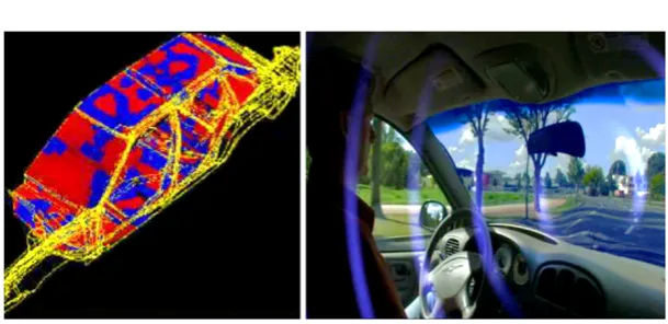
To model the propagation of acoustic waves inside a car, as illustrated in Figure1, the three-dimensional lossless wave equation is used, which can be obtained from the continuity equation (conservation of mass)
∂ρ˜
∂t + ∇(ρv)˜ =0, (1)
together with the Euler equations of fluid dynamics
˜
ρ
∂v
∂t +(v· ∇)v
= −∇ ˜p. (2)
Herev=v(x;y;z;t )is the particle velocity,ρ˜= ˜ρ(x;y;z;t )is the particle density, andp˜= ˜p(x;y;z;t )denotes the pressure, depending on Cartesian coordinatesx,y, zand timet. Under the simplifying assumptions that there is no temperature change, that the fluid is inviscid, that is, no shear forces occur, that the influence of external forces is restricted to those coming from displacements of the structure at the bound-aries, that the fluid is adiabatic, that is, there is no heat exchange during compression, that we have an ideal gas, that is,ρ= p
c2, wherecis the speed of sound, and finally that(v· ∇)vandρ∂v∂t are small, we can make the Taylor expansions
˜
p=p0+p(x;y;z;t ), withp0p
p0=106p
,
˜
ρ=ρ0+ρ(x;y;z;t ), withρ0ρ.
Then from the Euler equation we obtain ρ0(∂v∂t)= −∇p or by differentiation
ρ0∇(∂v∂t)= −p, and from the continuity equation we get ∂ρ∂t +ρ0∇v=0. Alto-gether we obtain the highly simplified system of partial differential equations
1 c2
∂2p ∂t2 +ρ0∇
∂v
∂t =p+ρ0∇ ∂v
∂t =0
to which we have to add appropriate initial and boundary conditions. In a closed structure like the interior of the car, we can use the boundary conditions that are ob-tained from the displacement of the structure to obtain the fluid structure interaction, in an open structure like the acoustic waves emitted by the car to the outside, we have to incorporate appropriate far field conditions or transparent boundary conditions [5]. Letube the vector of displacements of the structure on the surface. Thenv=∂u∂t and thus with the outer normalνwe get
νρ0
∂2u
∂t2 = −ν∇p.
To obtain a variational formulation, we multiply the equations with a test functionw, and use integration by parts by integrating over control volumesV with surface ele-mentsS. This gives
V
1 c2w
∂2p ∂t2 dV+
V
(∇w)∇p dV = −ρ0
S
νw∂
2u
∂t2dS,
or equivalently
V
1 ρ0c2
w∂
2p
∂t2 dV +
V
1 ρ0
(∇w)∇p dV = −
S
νw∂
2u
∂t2 dS.
materials used inside the car, the surface geometry of the interior and this is also one of the terms, where the influence of the optimization is strong.
In the model treated here, damping and absorption was realized by an additional term
S
w r
ρ02c2
∂p ∂t dS,
wherer=r(α)is depending on the damping properties of the material (described by a parameter vectorα). We then obtain
V
1 ρ0c2
w∂
2
∂t2p dV +
S
w r
ρ02c2 ∂p ∂t dS+
V
1 ρ0
(∇w)∇p dV = −
S
νw∂
2u
∂t2 dS.
To this variational formulation we can directly apply finite element discretization in space. This leads (in time) to a second order system of implicit differential equations in descriptor form
Mfp¨d+Dfp˙d+Kfpd+Dsfu¨d=0, (3)
whereMf =MfT is a positive definite mass matrix,Kf =KfT is a positive definite
stiffness matrix, Df(α) is a symmetric positive semi-definite damping/absorption
matrix, andDsf describes the fluid structure coupling.
It should be noted that for the fluid model, the finite element discretization applied to the weak form of the partial differential equation is used. In contrast to this in the model describing the vibration of the structure, in industrial and engineering practice, typically a direct discrete finite element model is employed. This leads to one of the challenges that we will discuss below.
For the displacement vectorud in the different finite elements of the discretized
structure, assuming linear material laws, one directly obtains a linear second order system of differential-algebraic equations given by
Msu¨d+Dsu˙d+Ksud=fe+fp, (4)
wherefeis a (discrete) external load andfp is the pressure load. HereMsis a
sym-metric positive definite mass matrix, andDs is a symmetric positive semi-definite
damping matrix; both are real. The matrixKs has the formKs=K1(ω)+ıK2with
real symmetricK1,K2, where K1 is the positive semi-definite stiffness matrix. It
is often frequency dependent to model nonlinear material behavior. The matrixK2
models hysteretic damping, that is, damping that is proportional to the displacement (instead of the velocity), but is in phase with velocity [6]. Typically, the matrixK2is
of very small rank.
AlthoughMs is positive definite in theory, the matrix encountered in practice is
highly singular due to the fact that rotational masses are omitted. On the positive side, it is block diagonal with small blocks.
It remains to further discuss the coupling of the fluid part and the structure part of the system. The termfp originates from the pressure loadFp=
element modeling/discretization yieldsfp=DsfT pdand hence,
Msu¨d+Dsu˙d+Ksud−DTsfpd=fe. (5)
If we combine all the equations then we obtain a second order system of differential-algebraic equations
Ms 0
DsfT Mf ¨ ud ¨ pd +
Ds 0
0 Df ˙ ud ˙ pd +
Ks(ω)−DsfT
0 Kf
ud pd = fs 0 . (6)
Typically in this model the format ofMs is a factor 1,000-10,000 larger than the
for-mat ofMf, the mass and stiffness matrices are highly dependent on the geometry
and topology of the car, and the type of finite elements that are used. Since the struc-ture is essentially modeled with a fine (pretty much uniform) mesh, the matrices have dimensions of several millions. The stiffness matrix depends also on the material pa-rameters, while the damping and coupling matrices depend on geometry, topology and material parameters.
2 Results and discussion
2.1 Direct frequency response
Usually one of the first tasks in the analysis of acoustic fields is to solve the frequency response problem, that is, to simulate the behavior of the acoustic field under excita-tions (typically of the structure). The classical approach for the frequency response analysis of linear vibrational systems is to perform a Fourier ansatz
ud pd = ˆ u ˆ p
eıωt, fs= ˆf (ω)eıωt,
which then leads to a frequency dependent linear system of equations
−ω2
Ms 0
DsfT Mf
+ıω
Ds 0
0 Df
+
Ks(ω)−DsfT
0 Kf
ˆ u(ω) ˆ p(ω) = ˆ f (ω) 0 . (7)
This linear system, which (for a reasonable structure) has several millions of equa-tions, typically has to be solved for a large frequency rangeω=0, . . . ,1,000 Hz in small frequency steps and, depending on the type of excitation, for many right hand sides (load vectors).
Before we discuss solution methods let us introduce a useful modification of (7). For nonzero frequencies we may multiply the second block row byω−1and introduce the new variablev(ω)ˆ =ω−1p(ω). Then we obtain a new linear systemˆ
−ω2
Ms 0
0 Mf
+ıω
Ds ıDTsf
ıDsfT Df
+
Ks(ω) 0
0 Kf ˆ
u(ω)
ˆ
v(ω)
=
ˆ
f (ω) 0
,
(8)
which now has complex symmetric coefficients and, hence allows the use of memory-and flop-saving structured methods. To simplify notation, we write this as
P (ω)x(ω):=−ω2M+ıωD+K(ω)x(ω)=b(ω). (9) Since this system of equations has to be solved for many right hand sides and over a large frequency range, and all this within an optimization loop, a very efficient solver is necessary. This solver has to be able to recycle information from nearby problems (when stepping through the frequency range and modifying parameters in an optimization) and has to work efficiently in a modern multi-processor, multi-core hardware environment. Altogether, this is really a lot to ask for from a linear system solver and makes the use of black box solvers extremely difficult.
2.1.1 State-of-the-art in linear system solvers
Modern techniques for the solution of linear systems in industrial applications are typically a combination of methods, that use the best of each of the various available classes of methods.
The first class of methods are highly efficient direct solution methods that use Gaussian elimination with partial pivoting combined with other techniques from graph theory to achieve optimal performance, make efficient use of the sparsity structure to avoid fill-in, and save storage. Many of them are even implemented for the use on multiprocessor machines. Well known packages include UMFPACK [7], PARDISO [8], MUMPS [9], WSMP [10], or the HSL collection (for example, HSL_MA78 [11]) to name a few. In view of possibly many right hand sides they are a clear option, despite the fact that for the size and type of problems considered in industrial practice, the storage demands are so high that they typically can only work in an out-of-core setting, that is, the matrix factors are stored on hard disk instead of main memory. Another difficulty is that a new factorization has to be computed for every frequency or every modification in the optimization loop. Finally also the bad scaling and the fact that the problems get increasingly ill-conditioned for large fre-quencies presents a real challenge, because the desired solution accuracy may not be realizable. Some of the packages provide specialized routines for complex symmetric systems, which have the potential to half the storage and computational requirements, but may also increase the complexity of pivoting strategies.
method (QMR) [14]. A variant of the conjugate gradient method for complex sym-metric systems like (9) is CSYM [15]. In principle these methods would be very good candidates, since the linear systems are sparse and matrix vector multiplications are relatively cheap. Also, iffˆandK are independent ofω, then one can exploit the shift invariance property of Krylov subspaces [16,17]. However, oftenfˆor K do depend onωand without a good preconditioner the convergence of iterative methods (in particular for large frequencies) is dramatically slow or not realizable.
The third class of potential methods (exploiting the fact that there is a partial dif-ferential equation in the background) are multigrid or multilevel methods [18–20]. Unfortunately, despite the fact that they are efficiently used in the solution of wave propagation problems, such as Helmholtz or Maxwell equations [21], they cannot be used in a simple way in the described acoustic field problems, since the discrete FEM modeling of the structure does not provide a nice hierarchy of basis functions. If such a hierarchy was available then these methods would lead to very good precondition-ers for the Krylov subspace methods. However, with the current state of discrete FEM modeling (being engineering practice for decades) it is extremely difficult to incor-porate them into the current code solvers. This is even true for the algebraic multigrid methods like the Ruge-Stüben method [22] or hypre [23], due to the difficulty of hav-ing to solve for a large frequency range, many right hand sides and all this inside an optimization loop. It is needless to say that also the incorporation of these solvers in a multiprocessor, multi-core industrial software tool is another challenge.
The fourth class of methods which have made tremendous progress in the last decades are the adaptive finite element methods, see, for example, [24]. These refine the computational grid according to a priori and a posteriori error estimates and if implemented properly avoid globally fine meshes and therefore the extremely large linear systems and eigenvalue problems in the first place. However, the construction, analysis, and implementation of such methods for their use inside an industrial pack-age, including the treatment of a full frequency range and many right hand sides, is still in its infancy and requires a major research effort which fortunately is currently addressed in several research projects world-wide.
When our cooperation with SFE started, we essentially made the above analysis of the available methods and realized the following major obstacles.
• The problems are badly scaled and get increasingly ill-conditioned whenωgrows;
• for some parameter constellations the system becomes exactly singular with pos-sibly inconsistent right hand sides;
• typically there are many right hand sides;
• classical off-the-shelf iterative methods do not work well, or fail completely;
• direct solution methods have to work by storing the factors in out-of-core memory and cannot easily recycle information from previous frequency or optimization steps;
• no multilevel or adaptive grid refinement is applicable, the methods must be matrix based;
• the matricesM,K1are often slightly indefinite because of rounding errors during
2.1.2 What did we do?
With all the obstacles of the problem and all the deficiencies of the current meth-ods, the development and implementation of an appropriate linear solver for acoustic field frequency response problems is a major challenge. Furthermore, as in all in-dustrial projects, there was a deadline. In such a circumstance, the only possibility is to compromise between the optimality of a given method for a given problem, the provability of success, and the practical needs in the industrial environment.
Our compromise, since we had to deal with given matrices (as opposed to partial differential equations), was to develop and implement (in the SFE software environ-ment) a preconditioned subspace recycling Krylov subspace method which has the following features:
The initial search space for any frequencyωis chosen to contain the solutions for the last few frequencies, an approach also used in [25]. For the preconditioner, whose construction and application represent the dominant cost of the algorithm, we had to fulfill the requirement that it had to run in a distributive setting, store its results out-of-core, support complex arithmetic, in particular support complex symmetric systems. This is a tall order to ask for but fortunately we were able to base the preconditioner on existing software, using the complexLDLT factorization code of the MUMPS package [9]. The preconditioner was constructed from the symmetric real part of the linear system (9), that is, from
˜
P (ω):= −ω2
Ms 0
0 Mf
+
K1 0
0 Kf
.
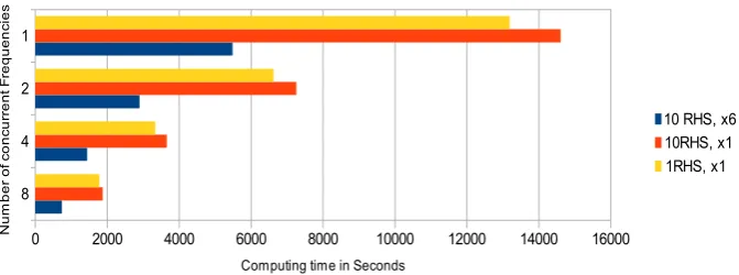
For small values ofωup to ca 60·2π corresponding to a frequency of 60 Hz, typ-ically only 3-6 iteration steps per frequency were necessary and the preconditioner could be kept unchanged for the whole frequency range. But the number of iteration steps per frequency grows substantially the largerωgets, so that more and more new preconditioners have to be computed. For large frequencies close to 1,000 Hz, the preconditioned Krylov method tends to be extremely slow or not convergent at all. As a consequence we constructed a hybrid method, where a certain frequency on-wards MUMPS is used as a direct solver for the system with the full matrixP (ω). Furthermore, it was decided to make use of the multi-core environment and to treat several linear systems simultaneously in a distributed fashion. One group of proces-sors solves the systems corresponding to the lower frequencies using the described iterative recycling method. Meanwhile, the other processor groups treat the high fre-quency systems with a full direct solve for each value ofω.
Fig. 2 Computation times of the described solver for 1, 2, 4, and 8 concurrent freqencies with different number of processors per frequency(×1 or×6)and different number of right hand sides (RHS).
2.1.3 Evaluation of our approach
Since there are commercial packages available, a question that may arise is why we need new numerical methods and solvers in the first place. From the point of view of the company SFE this is clear, they wanted their own solver in their product, and the solution method including the implementation was satisfactory for their needs. But in many respects the current methods are unsatisfactory from a scientific point of view. The discussed industrial problems present some of the current grant challenges in the field and the commercial packages are by no means able to solve these problems in a completely satisfactory way. To always get a more-or-less reasonable solution, and to be efficient, they often compromise for accuracy of the results which is certainly inadequate from a scientific point of view. Thus the cooperation with the industrial partner triggered new research questions for the academic world.
It became clear during the project that the concept ofrecyclingin iterative meth-ods, that is, the reuse of information that was already computed for other frequencies or in the course of an optimization procedure is not well-enough understood. As a consequence, motivated by the project with SFE, a new research project [26] in the DFG Research Center MATHEONwas started to further investigate the basic mathe-matical principles and to understand how they can be incorporated into new efficient methods [27].
2.2 Modal reduction
We have seen in the previous section that due to the fine mesh used for the discrete FEM modeling of the structure, the linear systems have very large dimensions. Typ-ically, however, one is interested in damping the low frequencies associated with the eigenvalues in the neighborhood of 0 (and the imaginary axis) of the complex sym-metric matrix function
Q(λ):=λ2M+λD+K=Q(λ)T, (10)
withM,D,K as in (9). The methods discussed below assume thatP is quadratic inλfor the eigenvalue computation, that is, the nonlinear dependency ofK on the frequency is ignored. One easily verifies that ifλ0is an eigenvalue ofQ(λ), that is,
P (λ0)x=0, thenxT is the corresponding left eigenvector but essentially no other
general properties of the eigenvalue problem are available, in particular, there is unfortunately no immediate variational property for the eigenvalues/eigenfunctions available, as there is for the undamped case [28].
Since one is interested only in part of the spectrum, a natural idea is to identify a space associated with eigenvectors and generalized eigenvectors associated with the important eigenvalues, and to project the problem into this subspace. This is amodel reductionapproach called modal reduction which, if efficiently implemented, can save a huge amount of computing time and storage, despite the fact that it is partially heuristic.
2.2.1 Complex symmetric quadratic eigenvalue problems
In view of the desire to do modal reduction, another task in the cooperation with SFE GmbH was the computation of a small number, say, eigenvalues in a trapezoidal region near zero, see Figure3(left), and the corresponding subspaceSspanned by
the eigenvectors and generalized eigenvectors associated with these eigenvalues, that is,S=span{s1, . . . , s}, where thesi form an orthonormal basis of this subspace,
that is,S= [s1, . . . , s]is an isometry.
The projected system would have the form
Q(λ):=λ2M+λD+K:=λ2STMS+λSTDS+STKS (11)
and would still be complex symmetric. In the context of model reduction, the require-ments for the reduced model are that the projected system is a good approximation to the large scale system for a large frequency range, and also for a large set of parame-ter variations. Furthermore, it has to be of small enough dimension, so that classical methods for nonlinear non-smooth optimization can be applied. Again this is a lot to ask, since currently for large scale problems there are really no methods available that guarantee to obtain all the eigenvalues of (10) in a specified region of the complex plane. For small dense problems one could employ the sign function method, [29, 30] but this would require storing full dense inverses of matrices of the given class, which is certainly not possible in the described acoustic field problems.
The currently used industrial techniques typically solve a simplified problem, for example, the eigenvalues and associated eigenvectors in the desired region for the undamped/uncoupled problem are used for the projection or an algebraic multilevel substructuring method (AMLS) is used that exploits the structure of the matrices as they arise form the discrete FEM [31]. All these techniques are partially heuristic, since there is no guarantee that all the desired eigenvalues are captured or that the eigenvalues from the projected system are close to those of the original physical sys-tem or of the FEM discretized syssys-tem, that is, in general, currently no error bounds are available. To generate such error bounds is a major challenge for the academic community and research in this direction has started in the project [32] with first results in [33,34].
Furthermore, the numerical solution of the large scale nonlinear eigenvalue prob-lem (10) itself also presents a mathematical challenge, for several reasons.
First of all the mass matrix is singular, so the problem has eigenvalues at∞which often cause convergence problems for the iterative methods, second of all, there are also several (typically six) eigenvalues at 0, corresponding to the six free degrees of motion, three each for translation and rotation, of the whole structure. In indus-trial practice the eigensolver is furthermore also often used for model verification, by checking whether there are exactly 6 eigenvalues at 0. Then, if the model is flawed, the singularity may be even higher.
2.2.2 What did we do?
Having assessed the various options and their potential advantages and drawbacks, we decided to develop a new method based on the following concepts and to imple-ment it into the SFE environimple-ment.
First of all, since the methods that work directly on the quadratic eigenvalue prob-lems, for example, [28,41,42], are not yet as mature as those for linear eigenvalue problems, the problem is linearized by introducing a new variableλxand turning (10) from a quadratic into a linear eigenvalue problem.
Since there is no method available that is guaranteed to find all eigenvalues in a region at feasible costs, we had to revert to a partially heuristic approach. We are looking for eigenvalues in the vicinity of target points which are scattered inside the region of interest. To find eigenvalues close to a particular targetσ, also called a shift, we use the shift-linearize-invert-ansatz [42] that requires computation of the largest eigenvalues of the matrix
A:=
Q(σ )−10
0 I
2σ M+D M
−I 0
.
This is done by the block Arnoldi method [43] which requires the application of the matrixAto given blocks of vectors during the generation of the Krylov subspace. This involves a solution of a linear system with the complex symmetric matrixQ(σ ). We again use the direct solver MUMPS to compute a complexLDLT factorization.
The block Arnoldi method searches for eigenvectors ofAwithin the block Krylov subspace
Km(A, B):=span
B,AB,A2B, . . . ,Am−1B, (12) which is known to contain, for increasingm, increasingly good approximations to eigenvectors corresponding to eigenvalues ofAof maximum absolute value - which correspond to the eigenvalues ofQ(λ)closest toσ. In the classical Arnoldi method, the starting block B is a vector. Otherwise, when B consists of several, say nb,
columns, the resulting method is the block Arnoldi method. The matrixB can be chosen in an (almost) arbitrary way, but if eigenvector or subspace approximations are known, the use of these will speed up convergence. Among the advantages of using the block method are that clusters of eigenvalues are handled better [44]. Fur-thermore, all vector-vector operations become matrix-matrix operations which can be implemented much more efficiently by use of BLAS level 3 routines [45] and the matrix-vector multiplication with the large matrixAcan be carried out with a block of vectors. Furthermore, the heuristic part of the algorithm is more reliable in the block case, see below.
In the actual implementation of the block Arnoldi algorithm the termsAiB are
never explicitly formed. Instead an orthonormal basis Qm = [V1, V2, . . . , Vm] of
Km(A, B) is generated by setting V1 to be an orthonormal basis of span(B)
fol-lowed by iteratively formingVi+1by orthonormalization ofAVi againstV1, . . . , Vi.
reflections [46,47] that are very stable and attain high efficiency by using BLAS-3 operations. Collecting all theVi and the orthonormalization coefficientsHi,j
re-sults in the well known Arnoldi relationAQm=QmHm+Vi+1Hm+1,mEmT with an
(m×m)-block Hessenberg matrixHm=(Hi,j)mi,j=1. The eigenvalues ofHm, called
Ritz values, are used as approximations of eigenvalues ofA. Likewise, the eigenvec-tors ofHm, multiplied withQm, are used as approximate eigenvectors ofA.
A drawback of the block Arnoldi method is the necessity to store the basisQm
which grows for increasingm. A typical way out of this problem is to restart the algorithm at some point. Instead of restarting with a single new starting block it is possible to restart with a whole Arnoldi relation. For the vector Arnoldi method, two such implicit restarting schemes are common, one using a filter polynomial [35] and one using a reordering of the Schur form ofHm[48]. We are using the latter approach
as the first one does not elegantly generalize to the block case [46].
The heuristic part of our method is that we assume that the block Arnoldi method really finds all eigenvalues in a circle around the shiftσ. While quite often the eigen-values do indeed appear and converge in the order of the distance to the shift, it is not rare that one or a group of eigenvalues converge slower than other farer away eigen-values. However, in these cases usually the missed eigenvalues are present as (yet) unconverged Ritz values. Therefore, we use the unconverged Ritz value that is closest to the shift as the radius of a circle that is trusted to contain no missed eigenvalues.
In the implementation, we repeatedly run the block Arnoldi method for different shifts, possibly several at once in a distributed setting. Figure3(right) shows the situ-ation after a few itersitu-ations. Large parts of the trapezoidal region are covered, leaving only some small remaining regions to be searched. New shifts are placed inside the largest such white regions, until the whole trapezoidal region of interest is covered by trusted circles.
Of course, with such a covering approach an eigenpair could be computed by more than one Arnoldi run for different shifts. For that reason the freshly discovered eigenpairs have to be checked for being copies of already previously found pairs. To achieve this we consider a new eigenpair(λ∗, x∗)being a copy, if [x∗T, λ∗x∗T]T is almost linearly dependent to the span of the vectors[xoldT , λoldxoldT ]T corresponding
to every known eigenvalueλoldsufficiently close toλ∗.
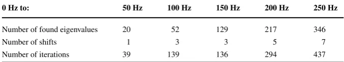
We applied the solver to a car model, discretized by a regular mesh of 35 mm lead-ing to 219,432 degrees of freedom. We were looklead-ing for eigenvalues within the trian-gle bordered by the lines Im(λ) >20 Re(λ), Im(λ) >−20 Re(λ), and Im(λ) < f·2π, forf∈ {50,100,150,200,250}. Table1lists the number of eigenvalues within these triangles, the number of used shifts, that is, used matrix factorizations, and the number of overall Arnoldi iterations, that is, matrix-block products. The test was performed on a PC with an Intel Core2 Duo E6850 CPU clocked at 3.0 GHz, with 4 GB RAM. One shift was addressed at a time using one processor. The block size was 5.
2.2.3 Evaluation of our approach
Table 1 Number of required shifts and iterations to find all eigenvalues between 0 and{50, . . . ,250}Hz.
0 Hz to: 50 Hz 100 Hz 150 Hz 200 Hz 250 Hz
Number of found eigenvalues 20 52 129 217 346
Number of shifts 1 3 3 5 7
Number of iterations 39 139 136 294 437
be kept out-of-core. Moreover, since the basis vectors are explicitly orthogonalized by a stable Householder scheme, the generated block Arnoldi basis is orthonormal to working precision. This is in sharp contrast to the basis generated by the non-symmetric Lanczos method which typically looses linear independence after enough iterations and leads to so-called spurious eigenvalues [49,50].
In our experiments the heuristic choice of the radii of trusted circles worked very well. In thousands of test cases with problems from SFE as well as randomly gen-erated problems, it happened only once that this approach missed an eigenvalue. This happened with a block size of one, that is, with the vector Arnoldi method. The method worked fine for this case if a block size of at lest two was used. In our implementation the default block size is 8.
Unfortunately, the improved robustness of the block-Arnoldi method compared with the standard Arnoldi method comes at the price of increased memory require-ments to store the basis. This downside is somewhat mitigated, however, by the use of restarts.
As another downside of our approach, so far only quadratic eigenvalue problems can be solved, for truly nonlinear problems withωdependence in K the methods is not directly applicable. On the other hand, the method can be applied to fluid or structure subsystems separately, or to the complete coupled system, and it tolerates a singular mass matrix.
3 Conclusions. The two-way street of industrial cooperation
But as we have discussed, already early on in the cooperation a lot of new research topics appeared that could not be treated within the current project (two-way-street). Examples include recycling methods for a sequence of slowly changing linear sys-tems, updating of preconditioners, guaranteed location of all eigenvalues inside a region of the complex plane, to name a few.
Competing interests
Our research was supported byDeutsche Forschungsgemeinschaft, via the DFG Research Center MATH
-EON, Mathematics for Key Technologies, in Berlin and by SFE GmbH, Voltastr. 5, 13355 Berlin.
Authors’ contributions
All authors participated in designing and implementing the solvers as well as in writing the manuscript. All authors read and approved the final manuscript.
Acknowledgements We thank H. Zimmer and A. Hilliges from our industrial partner SFE for the per-mission to use the figures obtained in the cooperation, and we thank Tobias Brüll, Elena Teidelt, Matthias Miltenberger for their help in the implementation. Moreover, we thank two anonymous referees for their valuable comments on a preliminary version of this paper.
References
1. ANSYS, Inc.: Programmer’s manual for ANSYS. http://www1.ansys.com/customer/content/ documentation/110/ansys/aprog110.pdf(2007)
2. MSC. Software Corporation: MSC.Nastran 2005 Installation and Operations Guide.http://www. mscsoftware.com/Products/CAE-Tools/MSC-Nastran.aspx(2004)
3. Antoulas, A.C.: Approximation of large-scale dynamical systems. In: Advances in Design and Con-trol, vol. 6. Society for Industrial and Applied Mathematics (SIAM), Philadelphia, PA (2005) 4. Benner, P., Mehrmann, V., Sorensen, D. (eds.): Dimension Reduction of Large-Scale Systems.
LNSCE, vol. 45. Springer, Heidelberg (2005)
5. Schmidt, F., Deuflhard, P.: Discrete transparent boundary conditions for the numerical solution of Fresnel’s equation. Comput. Math. Appl.29, 53–76 (1995)
6. Bishop, R.: The treatment of damping forces in vibration theory. Jl R. Aeronaut. Soc.59, 738 (1955) 7. Davis, T.A.: Algorithm 832: UMFPACK V4.3 - an unsymmetric-pattern multifrontal method. ACM
Trans. Math. Softw.30(2), 196–199 (2004)
8. Schenk, O., Gärtner, K.: Solving unsymmetric sparse systems of linear equations with PAR-DISO. Future Gener. Comput. Syst. 20(3), 475–487 (2004). http://www.sciencedirect.com/ science/article/B6V06-49NXY7J-F/2/e8260e5d8f19639019cddea4776c024c
9. MUMPS: MUltifrontal Massively Parallel Solver: Users’ Guide.http://graal.ens-lyon.fr/MUMPS
(2009)
10. Gupta, A.: WSMP: Watson Sparse Matrix Package, Part II. Direct solution of general sparse systems. IBM research report, IBM T. J. Watson Research Center.http://www.alphaworks.ibm.com/tech/wsmp
(2000)
11. Reid, J.K., Scott, J.A.: An efficient out-of-core multifrontal solver for large-scale unsymmetric ele-ment problems. Technical Report RAL-TR-2007-014, SFTC Rutherford Appleton Laboratory (2007) 12. Saad, Y., Schultz, M.H.: GMRES: a generalized minimal residual algorithm for solving nonsymmetric
linear systems. SIAM J. Sci. Stat. Comput.7(3), 856–869 (1986)
14. Freund, R.W., Nachtigal, N.M.: QMR: a quasi-minimal residual method for non-Hermitian linear systems. Numer. Math.60(3), 315–339 (1991)
15. Bunse-Gerstner, A., Stöver, R.: On a conjugate gradient-type method for solving complex symmetric linear systems. Linear Algebra Appl.287(1-3), 105–123 (1999)
16. Gu, G.D., Simoncini, V.: Numerical solution of parameter-dependent linear systems. Numer. Linear Algebra Appl.12(9), 923–940 (2005)
17. Simoncini, V., Perotti, F.: On the numerical solution of(λ2A+λB+C)x=band application to structural dynamics. SIAM J. Sci. Comput.23(6), 1875–1897 (2002) (electronic)
18. Hackbusch, W.: Multigrid Methods and Applications. Springer Series in Computational Mathematics, vol. 4. Springer-Verlag, Berlin (1985)
19. McCormick, S.F.: Multilevel Adaptive Methods for Partial Differential Equations. Frontiers in Ap-plied Mathematics, vol. 6. Society for Industrial and ApAp-plied Mathematics (SIAM), Philadelphia, PA (1989)
20. McCormick, S.F.: Multilevel Projection Methods for Partial Differential Equations. CBMS-NSF Re-gional Conference Series in Applied Mathematics, vol. 62. Society for Industrial and Applied Math-ematics (SIAM), Philadelphia, PA (1992)
21. Ernst, O.G.: Fast numerical solution of exterior Helmholtz problems with radiation boundary condi-tion by imbedding. Ph.D. thesis, Stanford University (1994)
22. Ruge, J.W., Stüben, K.: Algebraic multigrid. In: Multigrid Methods. Frontiers Appl. Math., vol. 3, pp. 73–130. SIAM, Philadelphia, PA (1987)
23. Falgout, R.D., Jones, J.E., Yang, U.M.: The design and implementation of hypre, a library of par-allel high performance preconditioners. In: Numerical Solution of Partial Differential Equations on Parallel Computers. Lect. Notes Comput. Sci. Eng., vol. 51, pp. 267–294. Springer, Berlin (2006). doi:10.1007/3-540-31619-1_8
24. Bangerth, W., Rannacher, R.: Adaptive Finite Element Methods for Differential Equations. ETH Lec-ture Series. Birkhäuser, Basel, Ch. (2003)
25. Fischer, P.F.: Projection techniques for iterative solution ofAx=bwith successive right-hand sides. Comput. Methods Appl. Mech. Eng.163(1-4), 193–204 (1998)
26. Numerical methods for large-scale parameter-dependent systems. Project C29, DFG Research Center Matheon, Berlin.http://www.matheon.de/research/show_project.asp?id=172
27. Gaul, A., Gutknecht, M.H., Liesen, J., Nabben, R.: Deflated and augmented Krylov subspace methods: Basic facts and a breakdown-free deflated MINRES. Preprint 749, DFG Research Center Matheon, Mathematics for key technologies, Berlin (2011)
28. Mehrmann, V., Voss, H.: Nonlinear eigenvalue problems: a challenge for modern eigenvalue methods. Mitt. der Ges. f. Angewandte Mathematik und Mechanik27, 121–151 (2005)
29. Bai, Z., Demmel, J.: Using the matrix sign function to compute invariant subspaces. SIAM J. Matrix Anal. Appl.19, 205–225 (1998). doi:10.1137/S0895479896297719(electronic)
30. Higham, N.J.: Functions of matrices. Theory and Computation. Society for Industrial and Applied Mathematics (SIAM), Philadelphia, PA (2008)
31. Bennighof, J.K.: Adaptive multi-level substructuring method for acoustic radiation and scattering from complex structures. In: Kalinowski, A.J. (ed.) Computational Methods for Fluid/Structure Inter-action, vol. 178, pp. 25–38. AMSE, New York (1993)
32. Adaptive solution of parametric eigenvalue problems for partial differential equations. Project C22, DFG research center Matheon, Berlin.http://www.matheon.de/research/show_project.asp?id=126] 33. Carstensen, C., Gedicke, J., Mehrmann, V., Miedlar, A.: An adaptive homotopy approach for
non-selfadjoint eigenvalue problems. Preprint 718, DFG Research Center Matheon, Mathematics for key technologies, Berlin (2010)
34. Miedlar, A.: Inexact adaptive finite element methods for elliptic PDE eigenvalue problems. Ph.D. thesis, Technische Universität Berlin, Inst. f. Mathematik (2011)
35. Lehoucq, R.B., Sorensen, D.C., Yang, C.: ARPACK Users’ Guide. Solution of Large-Scale Eigen-value Problems with Implicitly Restarted Arnoldi Methods. Software, Environments, and Tools, vol. 6. Society for Industrial and Applied Mathematics (SIAM), Philadelphia, PA (1998)
36. Saad, Y.: Numerical Methods for Large Eigenvalue Problems. Algorithms and Architectures for Ad-vanced Scientific Computing. Manchester University Press, Manchester (1992)
37. Schwetlick, H., Schreiber, K.: A primal-dual Jacobi-Davidson-like method for nonlinear eigenvalue problems. Internal Report ZIH-IR-0613, Techn. Univ. Dresden, Zentrum für Informationsdienste und Hochleistungsrechnen (2006)
39. Sleijpen, G.L.G., Booten, A.G.L., Fokkema, D.R., Van der Vorst, H.A.: Jacobi-Davidson type methods for generalized eigenproblems and polynomial eigenproblems. BIT Numer. Math.36(3), 595–633 (1996)
40. Sleijpen, G.L.G., Van der Vorst, HA: A Jacobi-Davidson iteration method for linear eigenvalue prob-lems. SIAM J. Matrix Anal. Appl.17(2), 401–425 (1996)
41. Beyn, W.: An integral method for solving nonlinear eigenvalue problems. ArXiv e-prints (2010) 42. Tisseur, F., Meerbergen, K.: The quadratic eigenvalue problem. SIAM Rev.43(2), 235–286 (2001) 43. Arnoldi, W.E.: The principle of minimized iteration in the solution of the matrix eigenvalue problem.
Q. Appl. Math.9, 17–29 (1951)
44. Lehoucq, R., Maschhoff, K.: Implementation of an implicitly restarted block Arnoldi method. Preprint MCS-P649–0297, Argonne National Laboratory, Argonne, IL (1997)
45. Dongarra, J.J., Croz, J.D., Hammarling, S., Duff, I.: A set of level 3 basic linear algebra subprograms. ACM Trans. Math. Softw.16, 1–17 (1990). doi:10.1145/77626.79170
46. Baglama, J.: Augmented block Householder Arnoldi method. Linear Algebra Appl.429(10), 2315– 2334 (2008)
47. Schreiber, R., Van Loan, C.: A storage-efficientW Yrepresentation for products of Householder trans-formations. SIAM J. Sci. Stat. Comput.10, 53–57 (1989)
48. Stewart, G.W.: A Krylov-Schur algorithm for large eigenproblems. SIAM J. Matrix Anal. Appl.23(3), 601–614 (2001/02)
49. Cullum, J., Willoughby, R.A.: Lanczos and the computation in specified intervals of the spectrum of large, sparse real symmetric matrices. In: Sparse Matrix Proceedings 1978 (Sympos. Sparse Matrix Comput., Knoxville, Tenn., 1978), pp. 220–255. SIAM, Philadelphia, Pa (1979)