Local Reduction in Physics
Joshua Rosaler
Abstract
A conventional wisdom about the progress of physics holds that succes-sive theories wholly encompass the domains of their predecessors through a process that is often called “reduction.” While certain influential accounts of inter-theory reduction in physics take reduction to require a single “global” derivation of one theory’s laws from those of another, I show that global re-ductions are not available in all cases where the conventional wisdom requires reduction to hold. However, I argue that a weaker “local” form of reduction, which defines reduction between theories in terms of a more fundamental no-tion of reducno-tion betweenmodels of a single fixed system, is available in such cases and moreover suffices to uphold the conventional wisdom. To illustrate the sort of fixed-system, inter-model reduction that grounds inter-theoretic re-duction on this picture, I specialize to a particular class of cases in which both models are dynamical systems. I show that reduction in these cases is under-written by a mathematical relationship that follows the broad prescriptions of Nagel/Schaffner reduction, and support this claim with several examples. Moreover, I show that this broadly Nagelian analysis of inter-model reduc-tion encompasses several cases that are sometimes cited as instances of the “physicist’s” limit-based notion of reduction.
1
Introduction
According to the most commonly told story about the progress of physics, suc-cessive theories in physics come ever closer to revealing the true, fundamental nature of reality. This convergence rests on the supposition that later theo-ries bear a special relationship to their predecessors often called “reduction,” which minimally requires one theory to encompass the domain of application of another. More specifically, the conventional wisdom tells us that Newto-nian mechanics “reduces to” special relativity, 1 special relativity to general
relativity, classical mechanics to quantum mechanics, quantum mechanics to relativistic quantum mechanics, relativistic quantum mechanics to quantum field theory, thermodynamics to statistical mechanics, and more. In order to assess the truth of the conventional wisdom, however, it is necessary to gain a
more precise sense of what is needed in a given case to show that one theory reduces to another.
In his widely cited 1973 paper, Nickles distinguished two types of ap-proach to reduction in physics: first, the apap-proach commonly employed by philosophers, which originates in Ernest Nagel’s well-known account of reduc-tion, and second, the approach commonly employed by physicists that requires one theory to be a “limit” or “limiting case” of another [25]. Since Nickles’ paper, these two accounts have tended to dominate philosophical discussion concerning issues of the general methodology of reduction in physics. As com-monly presented, both strongly suggest - and in some cases, state explicitly - that reduction between theories in physics should rest on a single “global” derivation of a high-level theory’s laws from those of a low-level theory. Here, I argue by means of a particular example that global reduction is not always available in cases where the conventional wisdom requires reduction to hold. However, I argue that it is possible to a define a weaker “local” notion of re-duction in physics that suffices to uphold the conventional wisdom by ensuring the subsumption of one theory’s domain by another. This notion of reduction is “local” in the sense that it permits the reducing theory to account for the reduced theory’s success through numerous context-specific derivations that are relativized to different systems in the high-level theory’s domain. These derivations concern the specificmodels that the theories use to describe a single fixed system, rather than the theories as a whole.
This paper has two main goals, which are mutually supporting. The first is to motivate and develop a local account of inter-theoretic reduction in physics. Inter-theoretic reduction in physics, understood minimally as the requirement that one theory subsume the domain of another, does not require anything as strong as global reduction directly between theories; local reduc-tion suffices for this purpose, and moreover avoids difficulties that afflict global approaches. I then argue that local reduction between theories should be un-derstood in terms of the more basic notion of reduction between models of a single fixed system. The second goal is to illustrate what is meant by fixed-system, inter-model reduction by giving an account of this concept in a special class of cases where both models of the system in question are dynamical sys-tems, and to show that such cases can be analyzed in terms of a certain model-based adaptation of the Nagel/Schaffner approach to reduction. I further show that this broadly Nagelian analysis of inter-model reduction encompasses many cases that have been cited as instances of “physicists’” limit-based notion of reduction, as well as providing a more precise characterization of these cases than do existing formulations of the limit-based approach. Finally, I suggest how this model-based adaptation of the Nagel/Schaffner approach might be extended to fixed-system, inter-model reduction involving models that are not dynamical systems.
2 and 3, is largely non-technical and concerns issues of general methodology. As suggested, its purpose is to motivate and present a certain local, model-based approach to inter-theoretic reduction and to explain how this strategy avoids certain difficulties that afflict more global approaches. In Section 2, I briefly review two approaches to reduction global Nagelian and global limitbased -that are often taken as the focus of philosophical discussions of inter-theoretic reduction in physics, and highlight some of their limitations. In Section 3, I sketch a local approach to inter-theoretic reduction in physics that relies on the more basic notion of fixed-system reduction between models and respond to one major objection that such an approach is likely to elicit.
Part II, which consists of Sections 4, 5 and 6, provides a detailed techni-cal analysis of fixed-system, inter-model reduction in a particular set of cases where both models of the system in question are dynamical systems, as well as briefly discussing possible expansions of this analysis to fixed-system, inter-model reduction involving other types of inter-model. Section 4 describes a gen-eral mathematical relationship between dynamical systems models that serves to underwrite many real instances of fixed-system, inter-model reduction in physics. In a certain strong sense, this mathematical relationship constitutes an application of the criteria for Nagel/Schaffner reduction to the context of fixed-system, inter-model reduction between dynamical systems models. Sec-tion 5 shows how this general relaSec-tionship serves to characterize reducSec-tion across a wide range of particular cases, and to subsume a number of cases that are commonly cited as examples of the physicist’s limit-based notion of re-duction. Section 6 briefly discusses possibilities for extending and generalizing this strategy for inter-model reduction beyond the set of cases discussed here: first, to an analysis of the relationship between symmetries of the two models involved in a reduction, and second, to an analysis of cases where one or both of the models involved in the reduction is not a dynamical system but some other kind of model (e.g., stochastic, non-dynamical, etc.).
The distinct portions of the analysis given in Parts I and II complement each other in a number of important ways. Part I serves to frame the analysis of reduction between dynamical systems given in Part II within a more general picture of inter-theoretic reduction and in particular to situate this analysis relative to the two accounts of inter-theoretic reduction in physics first distin-guished by Nickles. By the same token, Part II provides a concrete illustration of the sort of fixed-system, inter-model reduction that is taken as the basis for the local approach to inter-theoretic reduction described in Part I.
1.1
A Few Points of Terminology
Before proceeding, it is worth taking a moment to clarify several points of terminology.
I do not attach my usage to any specific account of reduction - e.g., Nagelian, limit-based, New Wave, functionalist. Rather, I use it to designate a certain general concept that, I take it, all, or most, of the many specific accounts aim to make more precise. “Reduction,” then, is taken to designate the general requirement that two descriptions of the world “dovetail” in such a manner that one description entirely encompasses the range of successful applications of the other. That is, reduction on this usage requires subsumption of one description’s domain of applicability by the other, while the specific sense in which the two descriptions “dovetail” in order to achieve this is deliberately left vague, so as not to bias its usage toward any particular account.
As Nickles has noted, the usage of the term “reduction” most common among philosophers takes the less accurate and encompassing description in a reduction to “reduce to” the more accurate and encompassing description, whereas the usage most common among physicists takes the more accurate, encompassing description to “reduce to” the less accurate and encompassing description. In what follows, I will always adopt the philosopher’s convention, even when discussing the physicist’s limit-based notion of reduction, so that if theory T2 is a “limiting case” of T1, we will say that T2 “reduces to” T1.
I will also reserve the term “high-level” to refer to the description that is purportedly reduced and “low-level” to refer to the description that pur-portedly does the reducing. This usage generalizes another use of the “high-level/low-level” distinction, which presupposes that the high-level description is in some sense a coarse-graining of the low-level description, or that the high-level description is in some sense “macro” and the low-level description in some sense “micro.” Here, no such assumption is made. For example, where the relation between Kepler’s and Newton’s theories of planetary motion is concerned, Kepler’s theory would count on our usage as the “high-level” and Newton’s as the “low-level” theory even though Kepler’s theory is not in any normal sense a coarse-graining of Newton’s. While some authors have empha-sized the distinction between “inter-level” reductions (e.g. thermodynamics to statistical mechanics) and “intra-level” reduction (e.g. Newtonian mechanics to special relativity, or Kepler’s to Newton’s theory of planetary motion), the picture of reduction presented here does not rely on this distinction and treats both kinds of reduction on a par. 2
Henceforth, when I speak of “Nagelian” reduction, the reader should take this to refer specifically to the Nagel/Schaffner account of reduction, which allows for approximative derivations rather than requiring exact derivations. While Nagel/Schaffner reduction is widely framed within a syntactic view of theories as opposed to the semantic, modeltheoretic view adopted here -and is often taken to require global rather than local derivations, my use of the label “Nagelian” here does not presuppose these characteristics. Rather,
what is taken to be constitutive of “Nagelian” reduction on my usage is the general requirement that it be possible to derive, on the basis of the low-level description and through the use of bridge principles, approximate versions of the laws or constraints or equations that serve to characterize the high-level description. My usage does not presuppose any view as to whether theories are understood syntactically or semantically - although the specific local approach to reduction advocated here fits much more naturally with a semantic view. Moreover, my usage does not assume any commitments as to the particular nature of these bridge principles - such as whether they are to be understood as empirically established laws or definitions - apart from their role in enabling a translation or comparison between the frameworks of the two descriptions in question. Rather than taking the term “Nagelian” to designate a specific set of precisely defined formal requirements for reduction, I use it here to designate a certain broad strategy for reduction.
Since the local approach to inter-theoretic reduction that I describe here is grounded in a certain account of inter-model reduction, I should say some-thing about what I take to be the relationship between theories and models. For the purposes of this discussion, it will suffice to note that the manner in which any theory serves to describe a physical system in its domain is through some particular model of that theory. Moreover, the specification of any such model entails much narrower commitments than those that serve to charac-terize the theory itself. For example, specification of a particular quantum or classical model of a material object requires commitments to a particular form for the Hamiltonian (or force law or Lagrangian), including particular values for quantities like mass and charge, while the theories of quantum and classical mechanics themselves are compatible with many functional forms of the Hamiltonian and many values for these parameters. One of the central points of my discussion here is that it is sometimes not just the more gen-eral specifications that serve to characterize the high- and low-level theories in question that are relevant to underwriting the success of the high-level theory in a given case, but also the narrower, more context-dependent specifications that characterize the particular models of the two theories.
Part I: Local Reduction in Physics
method-ology of inter-theoretic reduction in physics very often seem to presuppose a global understanding of reduction. The goal of Part I of this article is to argue that insights about local reduction that have arisen in the general philosophy of science and philosophy of mind literatures ought to be imported into the analysis of reduction specifically within physics, and to suggest how this should be done.
In emphasizing a local approach to inter-theoretic reduction in physics, I do not mean to suggest that it is not possible to effect global reduction, or something approximating it, in some cases. Local reduction is weaker than global reduction and so includes global reduction as a special case. In fact, local reduction accommodates a whole spectrum of cases varying in the extent of their “global-ness”: for inter-theoretic reductions at the least global extreme of this spectrum, a separate derivation is required for each separate system in the domain of the high-level theory in order to effect the necessary subsumption of domains; at the most global extreme, it is possible to effect a fixed-system, inter-model reduction for every system in the high-level theory’s domain on the basis of a single derivation that applies uniformly across all such systems (and so does not depend essentially on details that characterize some systems but not others). In cases of inter-theoretic reduction that lie between these extremes, the derivations that underwrite fixed-system, inter-model reduction will rely on general results and mechanisms that apply across a wide range of systems, while also requiring reference to system-specific details at certain points in the derivation. An example of an inter-theoretic reduction at the global extreme of the spectrum is the reduction of Kepler’s theory of planetary motion (which consists of models that obey Keplter’s three laws) to Newton’s theory of gravitation. The domain of Kepler’s theory consists the motions of the various planets around the Sun (as well as other similar solar systems in the cosmos). Because the same general derivation connects models of Kepler’s theory to models of Newton’s theory irrespective of the particular planet in this domain that is being represented, the reduction of Kepler’s theory to Newton’s theory lies at the global end of the spectrum. On the other hand, not all inter-theoretic reductions required by the conventional “imperialist” view of the progress of physics admit of such global derivations, as I show explicitly in Section 3.1.
2
Nickles’ Two Senses of Reduction
theory’s laws from the low-level theory, rather than many separate derivations specialized to different contexts. This in turn suggests that it is the general assumptions characterizing the two theories, rather than the more specific de-tails characterizing the theories’ models of particular systems, that are relevant to showing how the low-level theory serves to encompass the high-level the-ory’s domain of success. Implicitly if not explicitly, these approaches seem to demand a global rather than a local form of reduction. While it is not impos-sible in some cases to interpret conventional formulations of both approaches as allowing for many local derivations, what can be said with relative definite-ness is that these formulations do not make the need for local derivations, or the fact these local derivations concern specific models of the theories rather than the theories themselves, at all explicit; and both of these points, I take it, do bear emphasizing explicitly. Moreover, as I discuss below, where the Nagel/Schaffner approach is concerned, the extensive philosophical literature that takes multiple realizability to preclude application of this approach does explicitly construe it as a global form of reduction.
2.1
Nagel/Schaffner Reduction
Reduction on the Nagel/Schaffner approach can be understood as a three-step process, starting with the basic ingredients of a low-level theoryTl, a high-level
theory Th, and a set of bridge principles (see, for example, [2] and [12]):
1. Derive an “image” theory Th∗ for some restricted boundary or initial conditions within the low level theoryTl. The “laws” of the image theory
Th∗ take the same form as the laws of Th, but relate quantities that are
defined using the terms and concepts of Tl.
2. Use bridge principles to replace terms in Th∗, which belong to the vo-cabulary of the low-level theory, with corresponding terms belonging to the high-level theory. This yields the “analogue” 3 theory T0
h. Like the
“laws” of Th∗, those of Th0 have the same form as the laws of Th, but
employ the terms and concepts of Th rather than of Tl.
3. If the analogue theory Th0 is ‘strongly analogous’ to the high level theory
Th, the high level theory has been reduced to Tl. The ‘strong analogy’
relation is sometimes also characterised as approximate equality, close agreement, or good approximation and can be understood in any of these senses.
Note that reduction on the Nagel/Schaffner approach does not require deriva-tion of the high-level theory’s laws themselves, but rather of some suitable ap-proximations to them. This is the key point that distinguishes Nagel/Schaffner
reduction from Nagel’s original approach. A further point worth noting is that there remains some dispute as to whether the bridge principles of Nagel/Schaffner reduction are empirically discovered laws or mere definitions, and whether they are biconditional or merely conditional relations. The popular term “bridge law,” which is often used to designate bridge principles, suggests a clear bias toward interpreting them as empirical laws; here, I use the term “bridge prin-ciple” so as to avoid the suggestion of bias toward any particular view on this matter.
2.2
Difficulties with Nagelian Reduction: Multiple
Re-alization
For a comprehensive review of, and response to, the many critiques that have been levelled against Nagelian approaches to reduction, Dizadji-Bahmani et al’s 2011 article “Who’s Afraid of Nagelian Reduction?” is excellent [12]. In the present context, I will focus exclusively on critiques grounded in multiple realization (MR) because such critiques have served as the major impetus for considering more local forms of reduction, particularly in the philosophy of mind and general philosophy of science literatures.
As its name suggests, multiple realization occurs when a single element of a high-level description (e.g., model, theory or whole science) is realized by more than one element of some lower-level description. A classic example from the philosophy of mind literature is the high-level psychological prop-erty of pain, which can be multiply realized in human brains, dog brains, badger brains and so on, all of which have different low-level biological (and physical) descriptions [27]. In the context of Nagelian reduction, realization of an element in the high-level theory by some element of the low-level the-ory is signified by means of a bridge principle. On many formulations of the Nagel/Schaffner approach, bridge principles are required to be bi-conditional identity statements identifying natural kinds in the high-level theory with nat-ural kinds in the low-level theory. But, as Fodor has argued, the best one can do in cases where multiple realization occurs is to identify the relevant concept in the high-level description with adisjunction of associated elements in the low-level description, and it is simply false in most cases that such a disjunction will be a natural kind of the low-level description (for example, in the sense that it occurs naturally in the laws or equations of the low-level theory)[16], [5]. In this manner, multiple realization typically precludes the ex-istence of bridge principles of the sort that are required by these formulations of Nagelian reduction.
there simply do not exist such global bridge principles. The unavailability of these bridge principles, in turn, precludes the possibility of the sort of global derivation required by global formulations of Nagelian reduction.
2.3
Limit-Based Reduction
On the limit-based approach to reduction, a high-level theoryTh reduces to a
low-level theory Tl if Th is a “limit” or “limiting case” of Tl. Somewhat more
precisely, Th reduces to Tl if there exists some set of parameters {i} defined
withinTl such that
lim
{i→0}
Tl=Th (1)
4 [25],[2]. Unlike Nagelian reduction, the notion of a limit-based approach
to reduction, as first explicitly identified by Nickles, seems to arise not from any clear-cut statement of the general requirements for this kind of reduction, but rather from an assortment of suggestive mathematical results, all of which involve or somehow gesture at the use of mathematical limits. It also seems to arise in part from a manner of speaking that is often employed in discus-sions of inter-theory relations in physics, as exemplified by references to the “nonrelativistic limit” of special relativity, the “classical limit” of quantum mechanics, the “thermodynamic limit” of statistical mechanics, the “geomet-ric optics limit” of wave optics, and so on. Various facets of this approach to reduction have been explored by many authors, including Batterman, But-terfield, Rohrlich, Berry, Ehlers, and Scheibe, among others [1], [7], [9], [28], [4], [14], [30], [31]. Recently, Norton has highlighted a role for limiting proce-dures in physics outside the context of reduction - specifically, in distinguishing between the activities of approximation and idealization and in fending off po-tential confusions caused by conflation of the two [26]. While it is clear that limits have a central role to play in our understanding of inter-theory relations generally, where reduction specifically is concerned, the vague and schematic relation lim{i→0}Tl = Th appears to be as close to a statement of general
criteria for limit-based reduction as has been given in the literature.
2.4
Difficulties with the Limit-Based Approach
Perhaps the most serious concern about the limit-based approach to reduction is that, in spite of its mathematical nature, it is extremely vague in its char-acterization of the general relationship that it takes to underwrite reduction. The expression lim{i→0}Tl =Th is not mathematically well-defined, as there
is no precise or general definition of what it is for one theory to be a limit or limiting case of another. Moreover, it is unclear from this expression whether
4Note that if one has lim
{i→∞}Tl=Th, or lim{i→a}Tl=Thwhere 0< a <∞, one can
the prescription to take the limit is to be understood literally or in some loos-ened sense. For example, if we are to understand the claim that Newtonian mechanics is the limit as vc →0 of special relativity literally, then the claim is patently false, since the limit of special relativity as vc →0 is a theory in which nothing moves, not Newtonian mechanics (assuming we take c, the speed of light, to be constant, as it is for all real physical systems). For this paradig-matic case to be regarded as an instance of limit-based reduction, it seems necessary to adopt a more liberal construal of the term “limit” - for example, by making use of first- or higher-order approximations in Taylor expansions in
v
c since strictly speaking, it is only thezero-th order term of such an expansion
gives the actual limit of this series as vc →0. In other cases, including discus-sions of the thermodynamic limit of statistical mechanics, where the number of degrees of freedom in a system is taken to infinity, the limiting process is interpreted literally - for example, when it is pointed out that the only way to recover the discontinuities of certain functions in thermodynamics from statis-tical mechanics is to literally take the limit as the number of degrees of freedom approaches infinity. Beyond the points of vagueness already mentioned, it is not clear on this approach which parts of Th and Tl must be related by these
“limits” in order for the relation lim{i→0}Tl=Th to hold; presumably, not just
any limiting relation between any two parts of the theories will do. Finally, limit-based approaches tend to differ on what constraints, if any, should be placed on the parameters i - for example, whether they are supposed to be
dimensionless, or may also be dimensionful constants of nature, for example. Given that this approach offers very little by way of precise characteriza-tions or clear commitments as to the nature of reductive relacharacteriza-tions in physics, it seems possible to take many cases that we might wish to characterize as suc-cessful reductions and categorize them as instances of limit-based reduction. But if existing formulations of the limit-based approach succeed at accom-modating many cases in physics, it is largely for the reason that they tell us so little, and are so vague, about the general requirements for reduction. It seems possible to count any reduction as an instance of limit-based reduction as long as the reduction somehow incorporates a procedure that may liberally be construed as “taking a limit.” The worry, then, is that this approach, at least in its existing formulations, may give the false impression of providing an authoritative, general account of reduction in physics in spite of having offered little by way of general insight beyond the assertion that, in cases of reduction,
something like a limit issomehow involved in the explanation of the high-level theory’s success on the basis of the low-level theory.
such a formulation is still vulnerable to worries about precisely the sort of vagueness that allows for this vast flexibility of interpretation.
3
Local Reduction in Physics
It was largely in response to critiques of global Nagel/Schaffner reduction that a number of authors, mostly in the philosophy of mind literature, were prompted to advocate for a more local approach to reduction in which a lower-level description accounts for the successes of a higher-level description through many context-specific derivations employing context-specific bridge principles, rather than through a single global derivation employing the same set of bridge principles for all systems in the high-level description’s domain. In partic-ular, Kim has argued that while multiple realization rules out “structure-independent” reductions of psychology to physical science, it does allow for “structure-specific” local reductions between these levels [22]. Following Kim, Dizadji-Bahmaniet al also have advocated a local response to anti-reductionist arguments from multiple realizability in the context of their general defence of Nagelian reduction [12]. Similar views can be found in the work of Church-land, Hooker, Schaffner, Enc and Lewis [11], Ch. 7; [20]; [29]; [15]; [23]; [5]. The main goal of the present analysis is show explicitly how this sort of local approach, which has been developed primarily in discussions about reduction in philosophy of mind and general philosophy of science, can be imported into methodological discussions of inter-theoretic reduction specifically within physics.
3.1
The Need for Local Reduction in Physics: An
Illus-trative Example
An example, concerning the relationship between classical and quantum me-chanics, will serve to make my general point that global reductions are not available in all cases where the conventional wisdom requires reduction to oc-cur, and that only a weaker and more local (but still highly non-trivial) form of reduction is available in such cases. As we will see, the source of trouble for global approaches to reduction in physics is that it is often not just the broad generalities characterizing the theories - which are common to all models of each of the theories - but also details that differentiate the various models of a given theory, that play a role in explaining why the high-level theory works in a given case. In short, system- or context-specific details often play an in-dispensable role in accounting for the high-level theory’s success on the basis of the low-level theory, and this precludes the sort of generality demanded by global forms of reduction.
also can be modelled, and modelled more accurately, in quantum mechanics.
5 Here, I will argue that any demonstration to this effect could not possibly,
even in principle, take the form of a global reduciton. Consider two systems in the domain of classical mechanics, both of which are described by the same classical model of a simple harmonic oscillator: the first system is a mass on a spring; the second is an electric charge of the same mass moving along a path bored through the axis of a uniform spherical charge distribution. (One can show that in the second case, there will be a restoring force on the charge that varies linearly with its distance from the center of the sphere.) Assume moreover that frictional/radiation effects can be ignored in both systems, and that the linear restoring force in both cases is characterized by the same ef-fective spring constant. Assuming that macroscopic bodies do belong to the domain of quantum mechanics, it is clear in this case that the quantum me-chanical models that serve to describe these two physical systems are going to be radically different from each other, and that the process of accounting for the success of the classical harmonic oscillator model on the basis of these quantum models is going to play out very differently in the two systems. In the second case, the classical potential generated by the electric field in the classi-cal model will be the same potential that appears in the Schrodinger equation of the underlying quantum model of the charge’s behavior. In the first case, the fact that one can employ a harmonic oscillator potential in the classical model in order to describe the motion of the block is something that needs to be explained in terms of the complex microscopic constitution of the spring -at the microscopic level, this potential will be wildly fluctu-ating on the length scale of the atoms and molecules making up the spring. A global reduction of classical to quantum mechanics is thus out of the question, since distinct derivations of the classical model’s success on the basis of the quantum model are required for each of the two systems.
While global reduction between classical and quantum mechanics fails in this case, there remains a non-trivial, and more local, sense of inter-theoretic reduction in physics, which I describe in the next section, that has the potential to accommodate this sort of example. One thing that people might - and, I take it, often do - mean by the claim that “classical mechanics reduces to quantum mechanics” is that every physical system whose behavior can be modeled in classical mechanics also can be modeled in quantum mechanics at least as accurately and in at least as much detail. This manner of construing the term “reduction” allows for the possibility that for each system separately, there is a direct relationship between the quantum and the classical modelof that system
that permits us to understand why the classical model succeeds at describing the system’s behavior given that the quantum model is the more detailed and accurate of the two descriptions. Arguments from multiple realization present no reason for doubting that such system-specific quantum-mechanical accounts of the success of classical mechanics are available in such cases.
3.2
A Local, Model-Based Approach to Inter-Theoretic
Reduction
The example just discussed suggests a local picture of inter-theoretic reduction in physics where reduction between theories may consist of many local, fixed-system reductions between models - which in turn may rely on assumptions specific to individual systems - rather than requiring a single global derivation that references only the broad generalities that characterize the theories as a whole. Let us provisionally suppose a notion of reduction between two models of a single fixed system,reductionM, whereby the low-level model accounts for
the success of the high-level model at tracking the behavior of the system in question; the nature of this relationship will be further illustrated in the second half of this paper through the detailed analysis ofreductionM in a particular
class of cases where both models are dynamical systems. Let us designate our local concept of reduction between theories reductionT, which we define as
follows:
Criteria for Local Inter-Theoretic Reduction: Theory Th
reducesT to theory Tl iff for every system K in the domain of Th
- that is, for every system K whose behavior is accurately repre-sented by some modelMh of Th - there exists a modelMl ofTl also
representing K such that Mh reducesM to Ml.
There are several crucial points to note about this local, model-based concept of inter-theoretic reduction. First, it presupposes a semantic understanding of theories as families of models, rather than a syntactic view which treats theories as axiomatic sets of propositions. Second, it is not simply a two-place relation between the theory Th and the theory Tl, but rather a three-place
relation between Th, Tl, and that class of real systems in the world that are
well-described by models of Th. Since reduction is understood here to require
that one description dovetail (in some appropriate sense) with another specif-ically in those cases where the reduced description works, some specification of the reduced description’s domain of success is required in order to assess whether any dovetailing between the theories is sufficient to underwrite the re-quired subsumption; here, the relevant dovetailing between theories generally occurs on a local level, between the different models that they use to describe systems in the high-level theory’s domain. Third, reductionM, characterized
broadly, requires that Ml furnish at least as accurate a description of K as
of approximation) K’s behavior. Fourth, the precise nature of relationship between models Mh and Ml that serves to underwrite reductionM in a given
case varies depending on the particular mathematical form of these models. Fifth, given the emphasis here on the distinction between theories and their individual models, it is also important to distinguish between what is meant here by the domain of a theory, on the one hand, and the domain of a model that the theory uses to describe a particular physical system. The domain of a single model of a theory, relative to some physical system K, consists of the set of circumstances under which the model accurately tracks the sys-tem’s behavior. The domain of a theory, as understood here, consists of the range of physical systems whose behavior is well-described (under some fairly robust range of circumstances) by some particular model of the theory, as well as the set of circumstances under which each of these models succeeds in tracking the behavior of the system that it describes. Sixth, the account
of reductionM that I develop in Part II for the particular case of reductions
between dynamical systems models follows, in a certain strong but qualified sense, the prescriptions of a localized Nagel/Schaffner approach. As I discuss in Section 6.2, the broadly Nagelian character of reductionM in the case of
dynamical systems likely extends to cases ofreductionM involving other kinds
of model as well. For this reason, the strategy for inter-theory reduction in physics described here can be understood as a local, model-based formulation of the Nagel/Schaffner approach.
3.3
A Worry about Local Reduction
The local approach to inter-theoretic reduction described in the last section addresses worries about multiple realization by allowing domain-relative, lo-cal derivations that employ context-specific bridge principles. One concern about this sort of move, however, is that in its acceptance of disjointed, local derivations of multiply realized high-level regularities, this strategy foregoes a certain legitimate demand forexplanation of MR - that is, an explanation that alleviates our sense of mystery as to how systems with such disparate low-level descriptions can all give rise to the same high-level regularity, presumably by identifying some salient commonality among them.
mathematical and conceptual frameworks of theories between which reduction is purported to hold, the task of understanding precisely how one and the same physical system can consistently be described by models of both theories simultaneously poses a significant enough challenge that it deserves not to be conflated with the task of explaining how multiple realization comes about. Reduction already has enough on its plate, so to speak. Indeed, there are many who doubt, and some, including pluralists like Cartwright and Dupre, who outright deny that it is possible to effect the sort of subsumption required by local approaches to reduction - that is, who deny the possibility of the sort of theoretical “imperialism” that seeks to include macroscopic systems like the moon within the domain of quantum mechanics, or thermodynamic systems within the domain of statistical mechanics [10], [13]. Local reduction facilitates such imperialism, but without providing the sort of explanation of multiple realization that is sometimes called for.
Having made these remarks, it is worth pointing out that a good deal of important philosophical analysis has been done on the question of how to explain multiple realization in physics. In particular, Batterman has noted that the phenomenon of universality in physics just is multiple realization, and that in physics one does find explanations of universality in the form of renormalization group analyses [3]. However, I emphasize again that this sort of issue is distinct from (though closely related to) the issue of how to effect the sort of theoretical subsumption required by reduction, and that it is only this latter issue that I seek to address here.
Part II: The Case of Dynamical Systems
My purpose in the second half of this paper is to illustrate more pre-cisely, through a specific class of cases, what is meant by “fixed-system, inter-model reduction” (“reductionM”) in the local picture of inter-theoretic
reduc-tion (“reductionT”) spelled out in Section 3.2. In the class of cases that I
consider here, both models of the system in question are dynamical systems models and, moreover, are assumed to share a common time parameter. In Section 4, I describe a general mathematical relationship, which I call “dy-namical systems reduction,” “DS reduction,” or “reductionDS,” that provides
a template for reduction between dynamical systems models across a wide range of cases, as I show explicitly with several examples in Section 5. More-over, I show in Section 4.4 that there is a strong sense in which DS reduction follows the broad prescriptions of Nagel/Schaffner reduction, albeit in a form adapted to the specialized context of fixed-system reduction between dynami-cal systems models. Part of the significance ofreductionDS is that it provides
one model can improve on the scope, detail and accuracy of another model in its description of a physical system, fully encompassing the latter model’s domain of application. It also serves to illustrate how models employing radi-cally different mathematical and conceptual frameworks can both consistently (within some margin of approximation) and accurately describe the behavior of one and the same physical system.
As I argue in Section 6, certain central features ofreductionDS can likely
be carried over to cases ofreductionM in which the models in question do not
meet the preconditions for reductionDS - for example, in cases of reduction
between dynamical systems models that do not share a time parameter, or in cases where one or both of the modelsMl andMh is stochastic (e.g., models of
Brownian motion, or of GRW quantum mechanics), or non-dynamical (e.g. the Ideal Gas Model), or where there is no global splitting of the space of possible solutions of the model into state spaces at different times. I also suggest how various features of DS reduction might be extended to provide an analysis of the relationship between symmetries of different models of the same system. I leave it to future work to give a more detailed analysis of reductionM in
such contexts. However, I argue in Section 7 that the strategy for reduction in these other cases is also likely to be Nagelian in the broad, liberalized sense described in Section 1.1. As was noted in the Introduction, one important general aspect of the approach to reduction adopted here is to begin narrowly by considering reduction in relatively specialized contexts and then consider what generalities can be drawn across ever wider ranges of cases, rather than demanding a high level of generality at the outset.
4
Fixed-System Reduction Between
Dynami-cal Systems Models
Dynamical systems models occur widely throughout physics: in Hamilto-nian models of relativistic and relativistic classical mechanics and non-relativistic and non-relativistic classical field theory, in Schrodinger picture models of non-relativistic quantum mechanics, relativistic quantum mechanics and quantum field theory, and in heat diffusion equations in thermodynamics, to name a few cases.
D(x, t1 +t2) for all x ∈ S and t1, t2 ∈ T [6]. For our purposes here, I will
further assume that S is a differentiable manifold endowed with a norm, that
T =R, thatDis continuous, and thatDis an invertible function ofxfor each timet. In dynamical systems that occur in physics, the evolution operatorDis usually determined by some set of first-order differential equations of motion,
dx
dt =f(x), (2)
wheref(x) is a continous function of x. The functionsf andD are related by the equation ∂t∂D(x0, t) =f(D(x0, t)). That is,D(x0, t) for fixedx0 specifies a
solution to the equation (2).
4.1
Reduction
Mfor Dynamical Systems
The analysis of reduction between dynamical systems provided in this section draws on the work of several authors. All explore variations on the notion that reduction between dynamical descriptions of a system requires commuta-tion between the operation of dynamical evolution and some other operation, such as coarse-graining, that maps elements of the low-level state space into elements in the high-level state space. More precisely, the thought is that application of the low-level dynamics for time t followed by application of the mapping from the low- to the high-level state space should approximately equal the result of first applying this mapping and then applying the high-level dynamics for timet. Wallace explores variations of this idea in the context of an investigation into the quantum-mechanical (specifically, Everettian) arrow of time [33]. 6 Giunti discusses this requirement in the context of reduction between dynamical systems generally, although the specific criteria that he imposes are too strong to apply to very many, if any, realistic cases in physics [18]. Yoshimi discusses a similar approach in the context of a general discussion about supervenience, with a view toward applications in philosophy of mind [35]. Butterfield suggests a formulation of this commutation condition that is quite similar to (but formulated independently of) Yoshimi’s, with a view to applications in physics; however, he points out a number of ways in which this condition may need to be weakened in order to be applied to realistic cases in physics [8]. The formulation of the commutation-based requirement for reduc-tion that I describe here differs from those of Wallace, Yoshimi and Butterfield in that it takes the high-level and the low-level models to be specified inde-pendently of each other, whereas on these other formulations the high-level dynamics are specificallydefined as the dynamics induced by the low-level dy-namics through some coarse-graining procedure. Giunti’s formulation, like the one suggested here, does take the high- and low-level models to be indepen-dently specified, though requires the operation connecting the state spaces of
the models specifically to be an injection and requires the commutation to be exact; both of these requirements preclude application to most realistic cases in physics. As I show in the next section, the formulation of the requirement that I present here is refined in such a way as to allow for broad application specifically to inter-model reduction in physics.
Assume, then, that two distinct dynamical systems modelsMh = (R, Sh, Dh)
and Ml = (R, Sl, Dl), which share a time parameter t, both serve to
de-scribe the same physical system K. (This is the case, for example, with non-relativistic and relativistic models of a proton, or between non-relativistic quantum-mechanical and relativistic quantum-field-theoretic models of an elec-tron, or between classical and quantum mechanical models of the center of mass of a golf ball, and in a wide range of other instances.) Assume, moreover, that
Mh succeeds at tracking the dynamical behavior of some subset of the degrees
of freedom characterizing system K within margin of error δ over timescaleτ
for initial conditions xh0 within some domain of states dh ⊂ Sh. Then define
the relationreductionDS as follows:
Mh reducesDS to Ml iff there exists a differentiable function
B : Sl → Sh that does not depend explicitly on time and a
nonempty subset dl ⊂ Sl in the domain of B such that dh ⊂
B(dl), and for any xl∈dl,
|B Dl(xl, t)
−Dh B(xl), t
|h <2δ, (3)
or more concisely,
B Dl(xl, t)
≈Dh B(xl), t
, (4)
for all 0≤t≤τ.
The notation | ◦ |h designates the norm on Sh, and the margin of error 2δ is
taken to be implicit in the ≈ of (4). Note that the expressionB Dl(xl, t)
on the left-hand side of (4) represents the trajectory on Sh induced by the
low-level dynamicsDl via the functionB, while the expressionDh B(xl), t
on the right-hand side of (4) represents the trajectory prescribed by the high-level dynamics for the initial condition B(xl)∈Sh. The mathematical relationship
between Mh and Ml specified byreductionDS thus requires that the function
B - let us call it a “bridge map” - commute with the operation of time evo-lution, where the time evolution is specified by the low-level dynamics if it comes before application of the bridge map and by the high-level dynamics if it comes after application of the bridge map. The requirement thatdh ⊂B(dl)
is imposed for the purpose of ensuring that all possible trajectories ofMh that
would accurately track the behavior of the relevant degrees of freedom of K
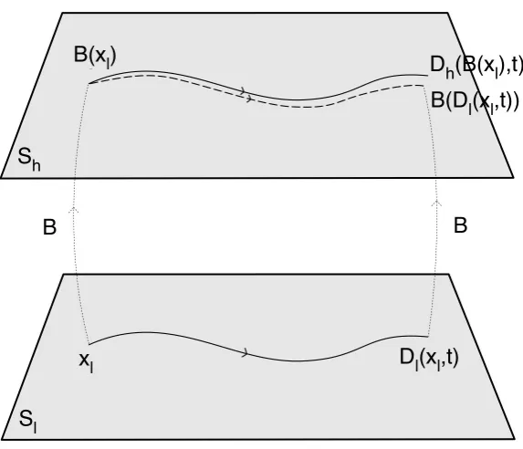
dynam-Figure 1: ReductionDS requires the existence of a time-independent “bridge map” B
from the state space of the low-level model, Sl, to that of the high-level model, Sh, that
approximately commutes with the operation of dynamical evolution for initial statesxl in
a certain domain dl ⊂ Sl. This amounts to the requirement that the trajectories on Sh
induced via B by the low-level dynamics approximate the trajectories prescribed by the corresponding high-level dynamics.
ics. In fact, in cases of reduction one expects the trajectory B Dl(xl, t)
to track the behavior of these degrees of freedom more accurately than the tra-jectoryDh(B(xl), t) if the low-level model Ml is the more accurate of the two
descriptions. That is, we expect that over timescaleτ,B Dl(xl, t)
tracks the behavior of the relevant physical degrees of freedom ofK to within a margin of errorγsuch thatγ < δ. This in turn requires that the trajectoriesDh B(xl), t
and B Dl(xl, t)
agree with each other to within a margin of 2δ. Thus, the physical property of systemK that is represented byxh in the high-level model
is represented in the low-level model by B(xl), so that there is a strong sense
in which the high-level state and the function of the low-level state associated with the bridge mapco-refer in the range of contexts where both successfully track the behavior of the system. 7
I should clarify here that reductionDS is not being presented as a
essary or sufficient condition for reductionM in cases where two dynamical
systems sharing a time parameter are purported to describe the same phys-ical system (although I suspect that it does serve to characterize most such instances). It is not being put forward as a sufficient condition because, if the quantity B(xl) in the low-level model is supposed to stand in as the low-level
model’s surrogate for xh, one should expect it to mimicxh’s behavior in ways
other than through its dynamical evolution - for example, through its sym-metry transformation properties. This point is discussed further in Section 6.
ReductionDS is also not being put forward as a necessary condition in order to
leave open the possibility that there might be other ways in which dynamical systems models that share a time parameter and describe the same physical system may relate to each other so as to facilitate the kind of subsumption required of reduction. 8 Rather, the relation specified byreduction
DS is being
suggested here as atemplate for reduction that is useful for the treatment of a wide range of examples in this class of cases. Moreover, it suggests a strategy for reduction in some inter-model relations that are not as yet well-understood (e.g., between models of non-relativistic quantum mechanics and interacting quantum field theory, both of which can be formulated as dynamical systems using Schrodinger picture formulations) as well as suggesting extensions to inter-model reduction involving other kinds of model.
4.2
Reduction as a Three-Place Relation
I wish to address a concern about DS reduction that may occur to some readers: specifically, that given any two dynamical systems models in which the low-level state space has at least the same cardinality as the high-low-level one, the criteria for DS reduction will be satisfied trivially if we allowδto be sufficiently large, andτ and dh to be sufficiently small. This concern can be addressed by
highlighting the fact that it is not justany values ofδ,τ anddh are consistent
with the criteria for DS reduction; rather, these parameters are constrained by the nature of the fit between the model Mh and the behavior of the system K
itself. Recall that the parameterδserves to characterize the degree of accuracy with which Mh tracks the behavior of K; τ characterizes the timescales over
which it does so;dh characterizes the set of initial states for whichMh succeeds
in tracking the system’s behavior within this timescale and margin of error. Determining the values of these parameters is therefore an empirical matter, to be assessed on the basis of the observed fit between the high-level model and system. 9 Once we have fixed these parameters - or ranges of possible
values for them - the task of assessing whether the formal requirements of DS reduction are met for a given pair of models become a question purely of mathematics. Moreover, once these parameters have been set, the criteria for DS reduction represent a highly non-trivial constraint on the mathematical relationship between the two models.
It should be emphasized here that the two models Mh and Ml by
them-selves do not provide us with sufficient information to assess whether the re-quirements for DS reduction are met between them. A third element - namely, the system itself, and more specifically a comparison of the system’s behavior with the behavior prescribed by Mh - is needed in order to assess whether
the criteria for DS reduction are satisfied. This should come as no surprise since reductionM requires that the low-level model dovetail structurally with
the high-level model only in those circumstances where the high-level model “works” at tracking the behavior of the systemK. And, of course, the question as to what, precisely, these circumstances are is an empirical one requiring reference to the system itself.
The criteria for DS reduction reflect a more general approach to reduc-tion in which reducreduc-tion is, in a certain sense, regarded not as a two place relation between high- and low-level descriptions, but as athree-place relation between high-level description, low-level description and that portion of the physical world that both represent. This follows naturally from the particu-lar construal of “reduction” adopted here, which requires that the low-level description subsume the domain of application of the high-level description; in order to determine what this domain of application is, it is necessary to consider not only the descriptions themselves, but the quality and scope of agreement between the high-level description and the portion of the world it is supposed to represent.
4.3
“Differential” Conditions for DS Reduciton
Assume that the dynamics of the high- and low-level models are specified by first-order differential equations of the form (2), so that dxh
dt = fh(x, t) and 9Having said this, it is also important to acknowledge that it may not always be a simple matter to assess the precise parameters of agreement between our models and the systems they represent. Nevertheless, it is often possible at the very least to place empirically determinedbounds onδ,τ anddh. For example, we know that current models of quantum
dxl
dt =fl(x, t).
10 Then it is possible to state a stronger, “differential” version
of (4) that requires the low-level quantity B(xl) to approximately satisfy the
high-level equations of motion. Making the variable substitution x0h ≡ B(xl),
we can write this requirement compactily as
dx0h
dt ≈fh(x
0
h, t) (5)
or more explicitly as,
dB(xl(t))
dt ≈fh
B xl(t)
, t
. (6)
If this condition holds over timescaleτ and the margin of error characterizing the approximate equality in (6) is η, then condition (4) will be satisfied over timescale τ and within margin of error 2δ ≡ ητ. 11 As we will see in the
next section, in typical cases, the approximate equality (6) will continue hold only as long as xl(t) remains in some restricted domain d0l ⊂ Sl. Also, since
the validity of the relation (6) hinges on the behavior of B(xl(t)), which in
turn depends on the behavior ofxl(t), which in turn depends on the low-level
dynamical equations of motion, the condition (6) should be deduced from the low-level dynamics, together with the state restriction xl∈d0l.
4.4
DS Reduction as a Special Case of Local Nagel/Schaffner
Reduction
Recall that global Nagel/Schaffner reduction, described in Section 2, distin-guishes four ‘theories’: a low-level theory Tl, a high-level theory Th, an
“im-age” theory Th∗, and an “analogue” theory Th0. Th∗ is formulated in terms of the concepts of Tl and deduced directly from Tl, typically for some restricted
boundary or initial conditions. Th0 is then obtained from Th∗ by straightfor-ward bridge principle substitution, and is formulated in terms of the concepts of Th. If the reduction is successful, Th0 will be “strongly analogous” to Th,
where strong analogy signifies approximate agreement of some sort. DS reduc-tion, if effected through proof of the differential condition described in Section 4.3, follows essentially the same series of steps, but with models rather than theories.
By analogy with the four “theories” of global Nagel/Schaffner reduction, in DS reduction one has a low-level model Ml, a high-level model Mh, an
“image model” Mh∗ and an “analogue model” Mh0. The image model Mh∗ is formulated using elements of the modelMl - that is, in terms of mathematical
structures defined onMl’s state space - and can be deduced from Ml solely on
10Where, recall, ∂
∂tDh(xh0, t) =fh(Dh(xh0, t)) and ∂
∂tDl(xl0, t) =fl(Dl(xl0, t))
11To see this, integrate both sides of (6) fromt= 0 up to any timetless thanτ, employing the substitution fh(B(xl(t))) = ∂t∂Dh(B(xl0), t), the fact that B(Dl(xl0,0)) = B(xl0) =
the basis of a restriction to a particular domain of states in Sl. Its dynamics
are given by the relation,
“Image Model” Dynamics:
d
dtB xl(t)
≈fh B xl(t)
, t (7)
which holds for xl in some domain d0l ⊂ Sl. Note that this relation
approxi-mately takes the same form as the high-level equation of motiondxh
dt =fh(xh, t),
but with xh replaced by its counterpart B(xl) in the low-level model. Recall
from Section 4.3 that satisfaction of the image model dynamics within ap-propriate margins suffices to ensure satisfaction of the condition (4). The analogue modelMh0 is then obtained from the image model through the bridge map substitution,
Bridge Map Substitution:
x0h ≡B(xl) (8)
and the analogue dynamics are specified by the relation,
“Analogue Model” Dynamics:
dx0h
dt ≈fh(x
0
h, t). (9)
Note that this dynamical equation is identical to the high-level equation of motion, apart from the approximate nature of the given equality. The domain of applicability of this equation withinShis the image domainB(d0l). Note that
the expression B(xl), which occurs in the image model, is an expression built
from structures within the low level modelMl - in this sense, the image model
is formulated in the mathematical ‘language’ of the low-level model. On the other hand, the more condensed notation of the analogue model conceals the detailed construction ofx0hfrom quantities in the low-level modelMl, regarding
x0h simply as a point inSh rather than as a quantity constructed from elements
of Ml; in this sense, one may view the analogue model as formulated in the
mathematical ‘language’ of the high-level model. For reduction to take place, the analogue model Mh0 must be “strongly analogous” to the high level model
Mh. In DS reduction, the relationship of strong analogy is unambiguous, and
specifically requires that
x0h(t)−xh(t)
h <2δ ∀0≤t ≤τ, (10)
where τ again is the reduction timescale and the measure of approximation between the analogue and high-level dynamics is provided by the norm | ◦ |h
on the high-level state space. Note that this “strong analogy” claim is just the condition (3) rewritten using bridge map substitution x0h(t) ≡ B Dl(xl0, t)
and the definitionxh(t)≡Dh B(xl0), t
.
5
Examples of DS Reduction
In this section, I show that the conditions for DS reduction are satisfied by a range of different model pairs. I do so specifically by showing that the relation (6) holds for a certain choice of bridge map and a certain domain of states in the low-level state space, offering qualitative remarks concerning the timescale over which the relation (6) continues to hold. My presentation of each example will follow a common outline: a. specification of the state spaces and dynamical equations of the two models; b. specification of the bridge map between the models; c. specification of the domain d0l where Eq. (6) holds between the models; d. statement of the condition (6) for the particular pair of models being considered; e. restatement of this condition, in the form (5), which more directly resembles the high-level dynamical equation; f. discussion of factors affecting the timescale on which (6) holds. Where necessary, proof of (6) is deferred to the Appendix.
5.1
CM/QM
Let the high-level model Mh be a model of classical mechanics whose state
space is some N-particle, 6N-dimensional phase space Sh ≡ ΓN and whose
dynamicsDh are given by the solutions to the Hamilton equations (dXdt,dPdt) =
(∂H∂P,−∂H
∂X), with H = P2
2M +V(X). In the notation of Section 4.3, we have
xh ≡(X, P) and fh(xh)≡(∂H∂P,−∂H∂X) = (MP,−∂V∂X).
Let the low-level model Ml be a model of non-relativistic quantum
me-chanics whose state space is some N-particle Hilbert space Sl ≡ HN and
whose dynamics Dl are given by the solutions to the Schrodinger equation
i∂∂t|ψi = ˆH|ψi, with ˆH = 2MPˆ2 +V( ˆX). In the notation of Section 4.3, we have
xl≡ |ψi and fl(xl)≡ −iHˆ|ψi.
Consider the function B :HN →ΓN from the low-level to the high-level
state space that maps a quantum state into the phase space point associated with the expectation values of position and momentum in this state,
B(xl)≡(hψ|Xˆ|ψi,hψ|Pˆ|ψi) = (hXˆi,hPˆi). (11)
d0l≡ {|ψi ∈ HN||ψi=|q, pi for some q, p∈ΓN}, (12)
where|q, pidenotes a narrow wave packet with average positionq and average momentump, and the required standard of narrowness inX is defined relative to the scale of spatial variation of the potentialV. On the basis of the low-level Schrodinger dynamics, one can show that for |ψi in d0l, the relation (6) holds relative to this particular case, so that the quantity associated with the bridge map approximately satisfies the high-level Hamilton equations:
d
dt(hψ|Xˆ|ψi,hψ|Pˆ|ψi)≈ ∂H ∂P h
ψ|Xˆ|ψi,hψ|Pˆ|ψi
,−∂H
∂X
h
ψ|Xˆ|ψi,hψ|Pˆ|ψi
! = P M hˆ Pi
,−∂V(X)
∂X hˆ Xi ! , (13)
or, more compactly, employing the variable substitutions (X0, P0)≡(hψ|Xˆ|ψi,hψ|Pˆ|ψi),
d dt(X
0, P0)≈ ∂H
∂P
X0,P0
,−∂H
∂X
X0,P0 ! = P M P0
,−∂V(X)
∂X X0 . (14)
This claim follows straightforwardly from Ehrenfest’s Theorem, which states that dhdtPˆi = −h∂V∂Xˆ(X)i, from the fact that dhdtXˆi = MPˆ, and from the well-known result that for wave packets whose position-space width is narrow by comparison with the characteristic length scales on which V(X) varies,
dhPˆi
dt ≈ − ∂V(X)
∂X hˆ
Xi [24].
On timescales where wave packets remain ind0l, the relation (13) ensures that quantum expectation values of position and momentum approximately satisfy the classical dynamics of the high-level model, and that (4) is satisfied. These timescales in turn will depend on two general factors: 1) the maximum spread in position and momentum of wave packets allowed by the definition of
d0l, which in turn will depend on the required accuracy of the approximation in (13) and on the scale of spatial variation of the potentialV; 2) the dynamics of the low-level model, and in particular the mass M and the strength of chaotic effects associated with the Hamiltonian H. In general, the larger M is, the slower wave packets inHN will tend to spread; moreover, it is typically the case that the smaller the Lyapunov exponent characterizing chaotic divergences of trajectories in the classical phase space of the system, the slower the rate of spreading of wave packets inHN [36]. 12
5.2
NRQM/RQM
Let the high-level model Mh be a model of nonrelativistic quantum mechanics
of a spin-1/2 particle whose state space is the Hilbert space of 2-spinorsSh ≡ HP 13and whose dynamicsDh are given by the solutions to the Pauli equation,
i∂t∂φα(x, t) = 1
2m[σ·(ˆp−qA(x))] 2
+qV(x) αβφβ(x, t), where φα(x, t) are
2-spinor functions on 3-D space, α, β = 1,2, σi are the Pauli matrices, m is the
particle’s mass, q is its electromagnetic charge, and A(x) and V(x) are fixed background electromagnetic potentials. 14 In the notation of Section 4.3, we
havexh ≡φα(x, t) and
fh(xh)≡ −i 1
2m[σ·(ˆp−qA(x))] 2
+qV(x) αβφβ(x, t). 15
Let the low-level model Mlbe a model of relativistic quantum mechanics
for a spin-1/2 particle whose state space is the Dirac Hilbert space of 4-spinors
Sl ≡ HD and whose dynamics Dl are given by the solutions to the Dirac
equation i∂t∂ψa(x, t) =
α ·(−i∇ − q ~A(x)) + βm +qV(x)acψc(x, t), where
a= 1,2,3,4 and likewise forb and c, where repeated spinor indices have been summed over, αi and β are the Dirac matrices, m is the mass of the particle,
q is its electromagnetic charge, andA(x) and V(x) are fixed background elec-tromagnetic potentials. In the notation of Section 4.3, we have xl ≡ ψa(x, t)
and fl(xl)≡ −i
α·(−i∇ −q ~A(x)) +βm+qV(x)acψc(x, t). 16
Consider the function B :HD → HP from the low-level to the high-level
state space given by
B(xl)≡eimtPaαψa(x, t), (15)
wherePα
a is the projector onto the subspace of the 4-spinor space corresponding
to the upper two components of any spinor. Because of the time-dependent factor eimt, this bridge map may seem to violate the requirement that bridge maps not depend explicitly on time. However, the violation is only apparent
evolution of the molecule’s center of mass in some cases can be accurately described by the unitary evolution of a pure state (“bucky ball” interference experiments with large molecules have shown this explicitly, as discussed, for example, in [32], Ch. 6). The relatively large mass of such molecules by comparison with smaller particles like electrons, protons and neutrons slows the rate at which pure state wave packets spread, thereby allowing narrow wave packets to maintain their approximately classical evolutions over longer timescales in these systems. On such timescales, both the classical and quantum models are adequate to describe the motion of the molecule’s center of mass to within a certain reasonable margin of error.
13Where the “P” is for “Pauli.”
14Unless explicitly stated otherwise, I employ the Einstein summation convention over repeated indices throughout.
15 The reader should note that for purposes of concision, I am abusing notation here, since the statexh is not properly described by the componentsφα(x, t), but rather by the
expression xh ≡ |φi=PαR dx φα(x, t) |xαi, where |xαi is a state of positionx and spin
α(say, in the z-direction). Likewise, the expression forfh(xh) employs a similar abuse of
notation, as does my notation describing the low-level relativistic Dirac model.
since the state space is in fact theprojective Hilbert space, and multiplication of a Hilbert space vector in either the high-or low-level model by an overall phase (whether time dependent or not) does not affect the projective representation of the state. Now consider the domain of low-momentum 4-spinors,
d0l =
ψa(x)∈ HD
ψa(x) = X
i=1,2 Z µ
0
d3k ψ˜i(k)uai(k)e−ikx, µ m << 1
, (16)
where uai(k) are positive energy eigenstates of the Dirac Hamiltonian indexed by momentum k and the spin i, and the upper limit µ on the momentum integral imposes the restriction to low-momentum states. On the basis of the low-level Dirac dynamics, one can show that for ψa(x) ∈ d0
l, the relation
(6) holds for the given bridge map and models, so that B(xl) in this case
approximately satisfies the high-level Pauli equation:
∂
∂t e
imt
Paαψa(x, t)≈ −i
1
2m [σ·(−i∇ −qA(x))]
2
+qV(x)
αβ
eimtPaβψa(x, t)
(17)
or, more compactly, employing the variable substitutionφ0α(x, t)≡eimtPβ
aψa(x, t),
∂ ∂tφ
0α
(x, t)≈ −i
1
2m[σ·(−i∇ −qA(x))]
2
+qV(x)
αβ
φ0β(x) (18)
for all spatial positions x (not to be confused with the high-level state xh
or the low-level state xl). Proof of this relation can be found in [19], or in
most good textbooks on relativistic quantum mechanics, such as [24]. The timescales on which ψa(x, t) remains in d0
l will depend primarily on the choice
of background fields A(x) and V(x); the domain d0l will be preserved as long as these background fields do not transfer significant amounts of momentum (that is, on the order of m) to the spinor field.
5.3
NRQM/RQFT
Let the high-level model Mh be model of N free spinless particles in
non-relativistic quantum mechanics whose state space is some N-particle Hilbert space Sh ≡ HN and whose dynamics Dh are given by the solutions to the
non-relativistic Schrodinger equation for N free particles all with mass m:
i∂
∂tψ(x1, ..., xN, t) = − PN
i=1 1 2m∇
2
iψ(x1, ..., xN, t). In the notation of Section
4.3, we havexh ≡ψ(x1, ..., xN, t) and fh(xh)≡i PN
i=1 1 2m∇
2
iψ(x1, ..., xN, t). 17
Let the low-level model Ml be a model of a free massive scalar quantum
field in relativistic quantum field theory whose state space is the free-particle