SAT-Based Explicit LTLf Satisfiability Checking

(1)

The Thirty-Third AAAI Conference on Artificial Intelligence (AAAI-19)

SAT-Based Explicit

LTL

f

Satisfiability Checking

∗

Jianwen Li, Kristin Y. Rozier

Iowa State University

Ames, IA, USA {jianwen,kyrozier}@iastate.edu

Geguang Pu, Yueling Zhang

East China Normal University

Shanghai, China {ggpu,ylzhang}@sei.ecnu.edu.cn

Moshe Y. Vardi

Rice University Houston, TX, USA

[email protected]

Abstract

We present a SAT-based framework forLTLf (Linear Tem-poral Logic on Finite Traces) satisfiability checking. We use propositional SAT-solving techniques to construct a transition system for the inputLTLf formula; satisfiability checking is then reduced to a path-search problem over this transition system. Furthermore, we introduceCDLSC(Conflict-Driven

LTLf Satisfiability Checking), a novel algorithm that lever-ages information produced by propositional SAT solvers from both satisfiability and unsatisfiability results. Experimental evaluations show that CDLSCoutperforms all other exist-ing approaches forLTLf satisfiability checking, by demon-strating an approximate four-fold speed-up compared to the second-best solver.

Introduction

Linear Temporal Logic over Finite Traces, orLTLf, is a

for-mal language gaining popularity in the AI community for formalizing and validating system behaviors. While stan-dard Linear Temporal Logic (LTL) is interpreted on infi-nite traces (Pnueli 1977), LTLf is interpreted over finite

traces (De Giacomo and Vardi 2013). While LTL is typi-cally used in formal-verification settings, where we are in-terested in nonterminating computations, cf. (Vardi 2007),

LTLf is more attractive in AI scenarios focusing on finite

behaviors, such as planning (Bacchus and Kabanza 1998; De Giacomo and Vardi 1999; Calvanese, De Giacomo, and Vardi 2002; Patrizi et al. 2011; Camacho et al. 2017), plan constraints (Bacchus and Kabanza 2000; Gabaldon 2004), and user preferences (Bienvenu, Fritz, and McIlraith 2006; 2011; Sohrabi, Baier, and McIlraith 2011). Due to the wide spectrum of applications ofLTLf in the AI community (De

Giacomo, Masellis, and Montali 2014), it is worthwhile to study and develop an efficient framework for solving

LTLf-reasoning problems. Just as propositional

satisfiabil-ity checking is one of the most fundamental propositional reasoning tasks,LTLfsatisfiability checking is a

fundamen-tal task forLTLfreasoning.

Given an LTLf formula, the satisfiability problem asks

whether there is a finite trace that satisfies the formula. A

∗

A full report is at http://temporallogic.org/research/AAAI19/. Geguang Pu and Kristin Y. Rozier are corresponding authors. Copyright c2019, Association for the Advancement of Artificial Intelligence (www.aaai.org). All rights reserved.

“classical” solution to this problem is to reduce it to the LTL satisfiability problem (De Giacomo and Vardi 2013). The advantage of this approach is that the LTL satisfia-bility problem has been studied for at least a decade, and many mature tools are available, cf. (Rozier and Vardi 2007; 2010). Thus, LTLf satisfiability checking can benefit from

progress in LTL satisfiability checking. There is, however, an inherent drawback that an extra cost has to be paid when checking LTL formulas, as the tool searches for a “lasso” (a lasso consists of a finite path plus a cycle, representing an in-finite trace), whereas models ofLTLfformulas are just finite

traces. Based on this motivation, (Li et al. 2014) presented a tableau-style algorithm for LTLf satisfiability checking.

They showed that the dedicated tool,Aalta-finite, which con-ducts an explicit-state search for a satisfying trace, outper-forms extant tools forLTLfsatisfiability checking.

The conclusion of a dedicated solver being superior to

LTLf satisfiability checking from (Li et al. 2014), seems

to be out of date by now because of the recent dramatic improvement in propositional SAT solving, cf. (Malik and Zhang 2009). On one hand, SAT-based techniques have led to a significant improvement on LTL satisfiability check-ing, outperforming the tableau-based techniques of Aalta-finite(Li et al. 2014). (Also, the SAT-based toolltl2sat for

LTLfsatisfiability checking outperformsAalta-finiteon

par-ticular benchmarks (Fionda and Greco 2016).) On the other hand, SAT-based techniques are now dominant in symbolic model checking (Cavada et al. 2014; Vizel, Weissenbacher, and Malik 2015). Our preliminary evaluation indicates that

LTLf satisfiability checking via SAT-based model

check-ing (Bradley 2011; Een, Mishchenko, and Brayton 2011) or via SAT-based LTL satisfiability checking (Li et al. 2015) both outperform the tableau-based tool Aalta-finite. Thus, the question raised initially in (Rozier and Vardi 2007) needs to be re-opened with respect toLTLfsatisfiability checking:

is it best to reduce to SAT-based model checking or develop a dedicated SAT-based tool?

Inspired by (Li et al. 2015), we present an explicit-state SAT-based framework forLTLf satisfiability. We construct

theLTLf transition systemby utilizing SAT solvers to

(2)

specializing the transition-system approach of (Li et al. 2015) toLTLfand its finite-trace semantics, we get a

frame-work that is significantly simpler and yields a much more efficient algorithmCDLSCthan the one in (Li et al. 2015).

We conduct a comprehensive comparison among dif-ferent approaches. Our experimental results show that the performance of CDLSC dominates all other exist-ing LTLf-satisfiability-checking algorithms. On average,

CDLSCachieves an approximate four-fold speed-up, com-pared to the second-best solution (IC3 (Bradley 2011)+K-LIVE (Claessen and S¨orensson 2012)) tested in our experi-ments. Our results re-affirm the conclusion of (Li et al. 2014) that the best approach toLTLf satisfiability solving is via a

dedicated tool, based on explicit-state techniques.

LTL over Finite Traces

Given a setP of atomic propositions, anLTLf formula φ

has the form:

φ::=tt|p| ¬φ|φ∧φ| Xφ|φUφ;

wherett is true, ¬ is the negation operator, ∧ is the and operator,X is the strong Next operator and U is the Until operator. We also have the dualsff(false) fortt,∨for∧,N (weak Next) forX andRfor U. Aliteral is an atomp ∈ P or its negation (¬p). Moreover, we use the notationGφ (Globally) andFφ(Eventually) to representffRφandttUφ. Notably,X is the standardnextoperator, whileN isweak next; X requires the existence of a successor state, while N does not. ThusNφis always true in the last state of a finite trace, since no successor exists there. This distinction is specific toLTLf.

LTLf formulas are interpreted over finite traces (De

Gi-acomo and Vardi 2013). Given an atom set P, we define Σ = 2P be the family of sets of atoms. Letξ ∈ Σ+ _{be a} finite nonempty trace, withξ = σ0σ1. . . σn. we use|ξ| =

n+ 1to denote the length ofξ. Moreover, for0 ≤i ≤n, we denoteξ[i]as the i-th position ofξ, andξi to represent

σiσi+1. . . σn, which is the suffix ofξfrom positioni. We

• ξ|=φ1∧φ2, ifξ|=φ1andξ|=φ2; • ξ|=Xφif|ξ|>1andξ1|=ψ;

• ξ|= (φ1Uφ2), if there exists0 ≤i <|ξ|such thatξi |=

φ2and for every0≤j < iit holds thatξj |=φ1;

Definition 1(LTLf Satisfiability Problem). Given anLTLf

formula φover the alphabet Σ, we say φ is satisfiable iff there is a finite nonempty traceξ∈Σ+_{such that}_ξ_|₌_φ_.

Notations. We usecl(φ)to denote the set of subformulas of φ. LetA be a set ofLTLf formulas, we denote VAto

be the formula V

ψ∈Aψ. The two LTLf formulas φ1, φ2 are semantically equivalent, denoted as φ1 ≡ φ2, iff for every finite trace ξ, ξ |= φ1 iff ξ |= φ2. Obviously, we have (φ1 ∨φ2) ≡ ¬(¬φ1 ∧ ¬φ2), Nψ ≡ ¬X ¬ψ and (φ1Rφ2)≡ ¬(¬φ1U ¬φ2).

We say anLTLfformulaφis inTail Normal Form(TNF)

ifφis inNegated Normal Form(NNF) andN-free. It is triv-ial to know that everyLTLfformula has an equivalent NNF.

Assume φ is in NNF, tnf(φ) is defined as t(φ)∧ FT ail, whereT ailis a new atom to identify the last state of satisfy-ing traces (Motivated from (De Giacomo and Vardi 2013)), and t(φ) is an LTLf formula defined recursively as

fol-lows: (1)t(φ) = φif φistt,ff or a literal; (2) t(Xψ) = ¬T ail ∧ X(t(ψ)); (3) t(Nψ) = T ail ∨ X(t(ψ)); (4) t(φ1∧φ2) =t(φ1)∧t(φ2); (5)t(φ1∨φ2) =t(φ1)∨t(φ2); (6)t(φ1Uφ2) = (¬T ail∧t(φ1))Ut(φ2); (7)t(φ1Rφ2) = (T ail∨t(φ1))Rt(φ2).

Theorem 1. φis satisfiable ifftnf(φ)is satisfiable.

In the rest of the paper, unless clearly specified, the input

LTLf formula is in TNF.

Approach Overview

There is a Non-deterministic Finite Automaton (NFA)Aφ

that accepts exactly the same language as anLTLf formula

φ(De Giacomo and Vardi 2013). Instead of constructing the NFA for φ, we generate the correspondingtransition sys-tem(Definition 5), by leveraging SAT solvers. The transi-tion system represents an intermediate structure of the NFA, in which every state consists of a set of subformulas ofφ.

The classic approach to generate the NFA from anLTLf

formula, i.e., Tableau Construction (Gerth et al. 1995), cre-ates the set of all one-transition next stcre-ates of the current state. Since the number of these states can be extremely large, we leverage SAT solvers to compute the next states of the current state iteratively. Although both approaches share the same worst case (computing all states in the state space), our new approach is better for on-the-fly checking, as it com-putes new states only if the satisfiability of the formula can-not be determined based on existing states.

We show the SAT-based approach via an example. Con-sider the formula φ = (¬T ail ∧a)Ub. The initial state s0 of the transition system is {φ}. To compute the next states of s0, we translate φ to its equivalentneXt Normal Form (XNF), e.g.,xnf(φ) = (b∨((¬T ail ∧a)∧ Xφ)), see Definition 4. If we replace Xφ inxnf(φ)with a new propositions p1, the new formula, denoted xnf(φ)p, is a pure Boolean formula. As a result, a SAT solver can com-pute an assignment for the formula xnf(φ)p_{. Assume the}

assignment is {a,¬b,¬T ail, p1}, then we can induce that (a∧¬b∧¬T ail∧Xφ)⇒φis true, which indicates{φ}=s0 is a one-transition next state of s0, i.e.,s0 has a self-loop with the label{a,¬b,¬T ail}. To compute another next state of s0, we add the constraint ¬p1 to the input of the SAT solver. Repeat the above process and we can construct all states in the transition system.

Checking the satisfiability ofφis then reduced to finding a final state(Definition 6) in the corresponding transition sys-tem. Sinceφis in TNF, a final statesmeets the constraint thatT ail∧xnf(V_s₎p_(recall_s_{is a set of subformulas of}_φ_{) is}

satisfiable. For the above example, the initial states0is actu-ally a final state, asT ail∧xnf(φ)p_{is satisfiable. Because all}

(3)

conflict sequenceC, in which each element, denoted asC[i] (0≤i <|C|), is a set of states in the transition system that cannot reach a final state inisteps. Starting from the initial state, CDLSCiteratively checks whether a final state can be reached, and makes use of the conflict sequence to ac-celerate the search. Consider the formulaφ= (¬T ail)Ua∧ (¬T ail)U(¬a)∧(¬T ail)Ub∧(¬T ail)U(¬b)∧(¬T ail)Uc. In the first iteration,CDLSCchecks whether the initial state s0 = {φ} is a final state, i.e., whetherT ail∧xnf(φ)p is satisfiable. The answer is negative, sos0 cannot reach a fi-nal state in 0 steps and can be added into C[0]. However, we can do better by leveraging the Unsatisfiable Core (UC) returned from the SAT solver. Assume that we get the UC u1 = {(¬T ail)Ua,(¬T ail)U(¬a)}. That indicates every state scontaining u, i.e., s ⊇ u, is not a final state. As a result, we can adduinstead ofs0 intoC[0], making the al-gorithm much more efficient.

Now in the second iteration,CDLSCfirst tries to com-pute a one-transition next state ofs0that is not included in C[0]. (Otherwise the new state cannot reach a final state in 0 step.) This can be encoded as a Boolean formulaxnf(φ)p_∧

¬(p1 ∧ p2) where p1, p2 represent X((¬T ail)Ua) and X((¬T ail)U(¬a))respectively. Assume the new states1= {(¬T ail)Ua,(¬T ail)Ub,(¬T ail)U(¬b),(¬T ail)Uc} is generated from the assignment of the SAT solver. Then

CDLSCchecks whethers1can reach a final state in 0 step, i.e.,xnf(V_s

1)p∧T ailis satisfiable. The answer is negative and we can add the UCu2 ={(¬T ail)Ub,(¬T ail)U(¬b)} to C[0] as well. Now to compute a next state of s0 that is not included in C[0], the encoded Boolean for-mula becomes xnf(φ)p ∧ ¬(p1 ∧ p2) ∧ ¬(p3 ∧ p4) where p3, p4 represent X((¬T ail)Ub) and X((¬T ail)U(¬b)) respectively. Assume the new state s2 = {(¬T ail)Ua,(¬T ail)Ub,(¬T ail)Uc} is gen-erated from the assignment of the SAT solver. Since

xnf(V

s2)p ∧T ail is satisfiable,s2 is a final state and we conclude that the formulaφis satisfiable. In principle, there are a total of25 = 32states in the transition system ofφ, butCDLSCsucceeds to find the answer by computing only 3 of them (including the initial state).

CDLSCalso leverages the conflict sequence to acceler-ate checking unsatisfiable formulas. Like Bounded Model Checking (BMC) (Biere et al. 1999),CDLSCsearches the model iteratively, but BMC invokes only one SAT call for each iteration, whileCDLSC invokes multiple SAT calls.

CDLSCis more like an IC3-style algorithm, but achieves a much simpler implementation by using UC instead of the Minimal Inductive Core(MIC) like IC3 (Bradley 2011).

SAT-based Explicit-State Checking

Given an LTLf formula φ, we construct theLTLf

transi-tion system(Li et al. 2014; 2015) leveraging SAT solvers and then check the satisfiability of the formula over its cor-responding transition system.

LTL

f

Transition System

First, we show how one can consider LTLf formulas as

propositional ones. This requires considering temporal sub-formulas aspropositional atoms.

Definition 2(Propositional Atoms). For anLTLf formula

φ, we define the set of propositional atoms ofφ, i.e.,PA(φ), as follows: (1)PA(φ) = {φ} ifφ is an atom, Next, Until or Release formula; (2)PA(φ) = PA(ψ)ifφ = (¬ψ); (3) PA(φ) =PA(φ1)∪PA(φ2)ifφ= (φ1∧φ2)or(φ1∨φ2).

Considerφ= (a∧((¬T ail∧a)Ub)∧ ¬(¬T ail∧ X(a∨ b))). We havePA(φ) ={a, T ail,((¬T ail∧a)Ub),(X(a∨ b))}. Intuitively, the propositional atoms are obtained by treating all temporal subformulas of φ as atomic proposi-tions. Thus, anLTLf formulaφcan be viewed as a

proposi-tional formula overPA(φ).

Definition 3. For anLTLf formulaφ, letφp beφ

consid-ered as a propositional formula overPA(φ). Apropositional assignmentAofφp, is in2PA(φ)and satisfiesA|=φp.

Consider the formulaφ = (a∨(¬T ail∧a)Ub)∧(b∨ (T ail∨c)Rd). From Definition 3,φp_is₍_a_∨_p

1)∧(b∨p2) where p1, p2 are two Boolean variables representing the truth values of(¬T ail∧a)Uband(T ail∨c)Rd. Moreover, the set{¬a, p1((¬T ail∧a)Ub),¬b, p2((T ail∨c)Rd)}is a propositional assignment of φp_{. In the rest of the paper,}

we do not introduce the intermediate variables and directly say {¬a,(¬T ail ∧a)Ub,¬b,(T ail ∨c)Rd} is a proposi-tional assignment ofφp_{. The following theorem shows the}

relationship between the propositional assignment ofφpand the satisfaction ofφ.

Theorem 2. For an LTLf formula φand a finite trace ξ,

ξ |=φimplies there exists a propositional assignmentAof φp_{such that}_ξ_|₌V_A_{; On the other hand,}_ξ_|₌V_A_where Ais a propositional assignment ofφp, also impliesξ|=φ.

We now introduce theneXt Normal Form(XNF) ofLTLf

formulas, which is useful for the construction of the transi-tion system.

Definition 4(neXt Normal Form). AnLTLfformulaφis in

neXt Normal Form(XNF) if there are no Until or Release subformulas ofφinPA(φ).

For example,φ= ((¬T ail∧a)Ub)is not in XNF, while (b∨(¬T ail∧a∧(X((¬T ail∧a)Ub))))is. EveryLTLf

for-mulaφhas a linear-time conversion to an equivalent formula in XNF, which we denoted asxnf(φ).

Theorem 3. For anLTLf formulaφ, there is a

correspond-ing LTLf formula xnf(φ)in XNF such that φ ≡ xnf(φ).

Furthermore, the cost of the conversion is linear.

Observe that when φis in XNF, there can be only Next (no Until or Release) temporal formulas in the propositional assignment ofφp. Forφ=b∨(a∧ ¬T ail∧ X(aUb)), the setA ={a,¬b,¬T ail,X(aUb)}is a propositional assign-ment ofφp. Based onLTLf semantics, we can induce from

A that if a finite traceξsatisfying ξ[0] ⊇ {a,¬b,¬T ail} andξ1|=aUb,ξ|=φis true. This motivates us to construct the transition system forφ, in which{aUb}is a next state of {φ}and{a,¬b,¬T ail}is the transition label between these two states.

Letφbe an LTLf formula andA be a propositional

(4)

Definition 5. Given anLTLfformulaφand its literal setL,

letΣ = 2L. We define thetransition systemTφ= (S, s0, T) forφ, whereS ⊆2cl(φ)_{is the set of states,}_s

0={φ} ∈Sis theinitial state, and

• T : S × Σ → 2S is the transition relation, where s2 ∈ T(s1, σ)(σ∈ Σ) holds iff there is a propositional assignment A of xnf(V

s1)p such that σ ⊇ L(A) and

s2=X(A).

A run ofTφ on a finite trace ξ(|ξ| = n > 0) is a finite

sequences0, s1, . . . , snsuch thats0 is the initial state and

si+1∈T(si, ξ[i])holds for all0≤i < n.

We define the notation |r| for a run r, to represent the length of r, i.e., number of states inr. We say state s2 is reachable from states1 ini(i ≥ 0) steps (resp. in up to i steps), if there is a runron some finite traceξleading from s1tos2and|r|=i(resp.|r| ≤i). In particular, we says2is aone-transition next stateofs1ifs2is reachable froms1in 1 steps. Since a statesis a subset ofcl(φ), which essentially is a formula with the form ofV

ψ∈sψ, we mix the usage of

the state and formula in the rest of the paper. That is, a state can be a formula ofV

ψ∈sψ, and a formulaφcan be a set of

states, i.e.,s∈φiffs⇒φ.

Lemma 1. LetTφ = (S, s0, T)be the transition system of

φ. Every states∈Sis reachable from the initial states0.

Definition 6(Final State). Letsbe a state of a transition systemTφ. Thensis afinal stateofTφ iff the Boolean

for-mulaT ail∧(xnf(s))pis satisfiable.

By introducing the concept offinal state, we are able to check the satisfiability of theLTLfformulaφoverTφ.

Theorem 4. Letφbe anLTLfformula. Thenφis satisfiable

iff there is a final state inTφ.

An intuitive solution from Theorem 4 to check the satisfi-ability ofφis to construct states ofTφuntil (1) either a final

state is found by Definition 6, meaningφis satisfiable; or (2) all states inTφare generated but no final state can be found,

meaningφis unsatisfiable. This approach is simple and easy to implement, however, it does not perform well according to our preliminary experiments.

Conflict-Driven

LTL

f

Satisfiability Checking

In this section, we present a conflict-driven algorithm for

LTLf satisfiability checking. The new algorithm is inspired

by (Li et al. 2015), where information of both satisfiabil-ity and unsatisfiabilsatisfiabil-ity results of SAT solvers are used. The motivation is as follows: In Definition 6, if the Boolean for-mulaT ail∧xnf(s)p_{is unsatisfiable, the SAT solver is able}

to provide a UC (Unsatisfiable Core)csuch thatc ⊆sand T ail∧xnf(c)p_{is still unsatisfiable. It means that}_c_represents

a set of states that are not final states. By adding a new con-straint¬(V

ψ∈cXψ), the SAT solver can provide a model (if

exists) that avoids re-generation of those states inc, which accelerates the search of final states. More generally, we de-fine theconflict sequence, which is used to maintain all in-formation of UCs acquired during the checking process.

Definition 7 (Conflict Sequence). Given anLTLf formula

φ, a conflict sequence C for the transition system Tφ is a

finite sequence of set of states such that:

1. The initial states0={φ}is inC[i]for0≤i <|C|; 2. Every state inC[0]is not a final state;

3. For every states∈ C[i+ 1](0≤i <|C| −1), all the one-transition next states ofsare included inC[i].

We call eachC[i]is aframe, andiis theframe level.

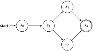
In the definition, |C|represents the length ofC andC[i] denotes the i-th element ofC. Consider the transition sys-tem shown in Figure 1, in which s0 is the initial state and s4 is the final state. Based on Definition 7, the se-quenceC = {s0, s1, s2, s3},{s0, s1},{s0}is a conflict se-quence. Notably, the conflict sequence for a transition sys-tem may not be unique. For the above example, the se-quence{s0, s1},{s0}is also a conflict sequence for the sys-tem. This suggests that the construction of a conflict se-quence is algorithm-specific. Moreover, it is not hard to in-duce that every non-empty prefix of a conflict sequence is also a conflict sequence. For example, a prefix ofCabove, i.e.,{s0, s1, s2, s3},{s0, s1}, is a conflict sequence. As a re-sult, a conflict sequence can be constructed iteratively, i.e., the elements can be generated (and updated) in order. Our new algorithm is motivated by these two observations.

s0

start s1

s2

s3

s4

Figure 1: An example transition system for the conflict se-quence.

An inherent property of conflict sequences is described in the following lemma.

Lemma 2. Let φbe an LTLf formula with a conflict

se-quenceCfor the transition systemTφ, thenT0≤j≤iC[j](0≤

i < |C|)represents a set of states that cannot reach a final state in up toisteps.

Proof. We first proveC[i](i≥0)is a set of states that cannot reach a final state inistep. Basically from Definition 7,C[0] is a set of states that are not final states. Inductively, assume C[i](i≥0)is a set of states that cannot reach a final state in isteps. From Item 3 of Definition 7, every states ∈ C[i+ 1]satisfies all its one-transition next states are inC[i], thus every states ∈ C[i+ 1]cannot reach a final state ini+ 1 steps. Now since C[i](i ≥ 0) is a set of states that cannot reach a final state ini steps,T

0≤j≤iC[j] is a set of states

that cannot reach a final state in up toisteps.

We are able to utilize the conflict sequence to accelerate the satisfiability checking ofLTLfformulas, using the

(5)

Theorem 5. TheLTLf formulaφis satisfiable iff there is a

runr =s0, s1, . . . , sn(n ≥0) ofTφsuch that (1) sn is a

final state; and (2)si(0≤i≤n) is not inC[n−i]for every

conflict sequenceCofTφwith|C|> n−i.

Proof. (⇐) Sincesnis a final state,φis satisfiable

accord-ing to Theorem 4. (⇒) Since φis satisfiable, there is a fi-nite trace ξsuch that the corresponding run r of Tφ on ξ

ends with a final state (according to Theorem 4). Letr be s0 −→ s1 −→ . . . sn wheresnis the final state. It holds that

si(0≤i≤n) is a state that can reach a final state inn−i

steps. Moreover for everyCofTφwith|C|> n−i,C[n−i]

(C[n−i]is meaningless when|C| ≤n−i) represents a set of states that cannot reach a final state inn−isteps (From the proof of Lemma 2). As a result, it is true thatsiis not in

C[n−i]if|C|> n−i.

Theorem 5 suggests that to check whether a statescan reach a final state inisteps (i≥1), finding a one-transition next states0ofsthat is not inC[i−1]is necessary; ass0 ∈ C[i−1]impliess0 cannot reach a final state ini−1steps (From the proof of Lemma 2). If all one-transition next states ofsare inC[i−1],scannot reach a final state inisteps.

Theorem 6. TheLTLfformulaφis unsatisfiable iff there is

a conflict sequenceC and i ≥ 0 such thatT

0≤j≤iC[j] ⊆

C[i+ 1].

Proof. (⇐) T

0≤j≤iC[j] ⊆ C[i + 1] is true implies that

T

0≤j≤iC[j] =

T

0≤j≤i+1C[j] is true. Also from Lemma 2 we knowT

0≤j≤iC[j]is a set of states that cannot reach

a final state in up to i steps. Since φ ∈ C[i] is true for eachi≥0,φis inT

0≤j≤iC[j]. Moreover,

T

0≤j≤iC[j] =

T

0≤j≤i+1C[j] is true implies all reachable states from φ are included inT

0≤j≤iC[j]. We have known all states in

T

0≤j≤iC[j]are not final states, soφis unsatisfiable.

(⇒) If φ is unsatisfiable, every state in Tφ is not a

fi-nal state. Let S be the set of states of Tφ. According to

Lemma 2, T

0≤j≤iC[j](i ≥ 0) contains the set of states

that are not final in up to i steps. Now we let C satisfy that T

0≤j≤iC[j](i ≥ 0) contains all states that are not

final in up to i steps, so T

0≤j≤iC[j] includes all

reach-able states fromφ, asφis unsatisfiable. However, because T

0≤j≤iC[j] ⊇

T

0≤j≤i+1C[j] ⊇ S(i≥ 0), there must be ani ≥ 0 such thatT

0≤j≤iC[j] =

T

0≤j≤i+1C[j], which indicates thatT

0≤j≤iC[j]⊆ C[i+ 1]is true.

Algorithm Design. The algorithm, named CDLSC

(Conflict-Driven LTLf Satisfiability Checking), constructs

the transition system on-the-fly. The initial states0 is fixed to be {φ} whereφ is the input formula. From Definition 6, whether a statesis final is reducible to the satisfiability checking of the Boolean formulaT ail∧xnf(s)p. Ifs0is a final state, there is no need to maintain the conflict sequence inCDLSC, and the algorithm can return SAT immediately; Otherwise, the conflict sequence is maintained as follows.

• InCDLSC, every element ofC is a set of set of subfor-mulas of the input formulaφ. Formally, eachC[i](i≥0)

can be represented by theLTLf formulaW_c∈C[i]

V

ψ∈cψ

wherecis a set of subformulas ofφ. We mix-use the no-tation C[i]for the corresponding LTLf formula as well.

Every statessatisfyings⇒ C[i]is included inC[i].

• C is created iteratively. In each iterationi ≥ 0, C[i] is initialized as the empty set.

• To compute elements inC[0], we consider an existing state s(e.g.,s0). If the Boolean formulaT ail∧xnf(s)pis un-satisfiable,sis not a final state and can be added intoC[0] from Item 2 of Definition 7. Moreover,CDLSCleverages the Unsatisfiable Core (UC) technique from the SAT com-munity to add a set of states, all of which are not final and includes, toC[0]. This set of states, denoted asc, is also represented by a set ofLTLfformulas and satisfiesc⊆s.

• To compute elements in C[i+ 1] (i ≥ 0), we consider the Boolean formula(xnf(s)∧¬X(C[i]))p_{, where}_X_(C[_i_])

represents the LTLf formula Wc∈C[i]

V

ψ∈cX(ψ). The

above Boolean formula is used to check whether there is a one-transition next state of sthat is not inC[i]. If the formula is unsatisfiable, all the one-transition next states ofsare inC[i], thusscan be added intoC[i+ 1]according to Item 3 of Definition 7. Similarly, we also utilize the UC technique to obtain a subsetcofs, such thatcrepresents a set of states that can be added intoC[i+ 1].

As shown above, every Boolean formula sent to a SAT solver has the form of (xnf(s)∧θ)pwheresis a state andθ is eitherT ailor¬X(C[i]). Since every statesconsists of a set ofLTLf formulas, the Boolean formula can be rewritten

asα1= (V_ψ∈sxnf(ψ)∧θ)p. Moreover, we introduce a new Boolean variablepψfor eachψ∈s, and re-encode the

for-mula to beα2 =V_ψ∈spψ∧(V_ψ∈s(xnf(ψ)∨ ¬pψ)∧θ)p.

α2is satisfiable iffα1is satisfiable, andAis an assignment ofα2iffA\{pψ|ψ∈s}is an assignment ofα1. Sendingα2 instead ofα1 to the SAT solver that supports assumptions (e.g., Minisat (E´en and S¨orensson 2003)) enables the SAT solver to return the UC, which is a set ofs, whenα2is un-satisfiable. For example, assumes = {ψ1, ψ2, ψ3}andα2 is sent to the SAT solver with{pψi|i∈ {1,2,3}}being the

assumptions. If the SAT solver returns unsatisfiable and the UC{pψ1}, the setc ={ψ1}, which represents every state

includingψ1, is the one to be added into the corresponding C[i]. We use the notationget uc()for the above procedure.

(6)

Algorithm 1Implementation ofCDLSC

Require: AnLTLfformulaφ. Ensure: SAT or UNSAT.

1: ifT ail∧xnf(φ)p_{is satisfiable}_then

2: return SAT; 3: SetC[0] :={φ}; 4: Setf rame level:= 0; 5: whiletruedo

6: iftry satisf y(φ, f rame level)returns truethen

7: return SAT;

8: ifinv f ound(f rame level)returns truethen

9: return UNSAT;

10: f rame level:=f rame level+ 1; 11: SetC[f rame level] =∅;

implemented recursively. Each time it checks whether a next state of the inputφ, which belongs to a lower level (than the inputf rame level) frame can be found (Line 2). If such a new stateφ0is constructed,try satisf yfirst checks whether φ0 is a final state whenf rame level is 0 and returns true if so. Ifφ0 is not a final state, a UC is extracted from the SAT solver and added toC[0](Line 5-11). Iff rame level is not 0,try satisf yrecursively checks whether a model of φ0 can be found with the length off rame level (Line 12-13). If the result is negative and such a state cannot be con-structed, a UC is extracted from the SAT solver and added intoC[f rame level+ 1](Line 14-15).

Algorithm 2Implementation oftry satisf y Require: φ: The formula is working on;

f rame level: The frame level is working on.

Ensure: true or false.

1: Letψ=¬X(C[f rame level]); 2: while(ψ∧xnf(φ))p_{is satisfiable}_do

3: LetAbe the model of(ψ∧xnf(φ))p_;

4: Letφ0 =X(A), i.e., be the next state ofφextracted fromA;

5: iff rame level== 0then

6: if T ail∧xnf(φ0)p_{is satisfiable}_then

7: return true;

8: else

9: Letc=get uc();

10: AddcintoC[f rame level]; 11: Continue;

12: iftry satisf y(φ0, f rame level−1)is truethen

13: return true; 14: Letc=get uc();

15: AddcintoC[f rame level+ 1]; 16: return false;

Notably, Item 1 of Definition 7, i.e.,{φ} ∈ C[i], is guar-anteed for each i ≥ 0, as the original input formula of try satisf yis alwaysφ(Line 6 in Algorithm 1) and there is somec(Line 15 in Algorithm 2) including{φ}that is added intoC[i], if no model can be found in the current iteration.

The procedure inv f ound in Algorithm 1 implements Theorem 6 in a straightforward way: it reduces checking

0

5000

10000

15000

20000

0 1000 2000 3000 4000 5000 6000 7000

Aalta-finite ltl2sat Aalta-infinite IC3+K-LIVE CDLSC

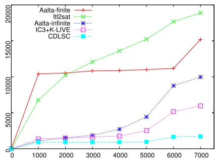
Figure 2: Result forLTLf Satisfiability Checking on

LTL-as-LT Lf Benchmarks. The X axis represents the number

of benchmarks, and the Y axis is the accumulated checking time (s).

whether T

0≤j≤iC[j] ⊆ C[i + 1] holds on some frame

level i, to satisfiability checking of the Boolean formula V

1≤j≤iC[j] ⇒ C[i+ 1]. Theorem 7 provides the

theoret-ical guarantee thatCDLSCalways terminates correctly.

Lemma 3. After each iteration ofCDLSCwith no model found, the sequence C is a conflict sequence ofTφ for the

transition systemTφ.

Theorem 7. TheCDLSCalgorithm terminates with a cor-rect result.

Summarily,CDLSCis a conflict-driven on-the-fly satis-fiability checking algorithm, which successfully leads to ei-ther an earlier finding of a satisfying model, or the faster termination with the unsatisfiable result.

Experimental Evaluation

Benchmarks1 _{Our extensive experimental evaluation,}

checking 9142 formulas, uses two classes of benchmarks: 7442 LTL-as-LT Lf (since LTL formulas share the same

syntax as LT Lf) and 1700 LT Lf-Specific benchmarks,

which are common LT Lf patterns that are all satisfiable

by finite traces (but not necessarily by infinite traces). We check both execution time and correctness; checking also correctness, as in (Rozier and Vardi 2007), ensures we are comparing performance of tools finding thesameresults.

LTL-as-LT Lf benchmarks consist of the following. Random Formulas generated as in (Rozier and Vardi 2011), vary the number of variables {1, 2, 3}, formula length {5, . . . , 100}, and probability of choosing a tem-poral operator {0.3,0.5,0.7,0.95} from the operator set {¬,∨,∧,X,U,R,G,F,GF }. We generate all formulas prior to testing for repeatability. Counter Formulasscale four, temporally complex patterns that describe large state

1

(7)

Type Number Result IC3+K-LIVE Aalta-finite Aalta-infinite ltl2sat CDLSC

Alternate Response 100 sat 134 1 48 123 3 Alternate Precedence 100 sat 154 3 70 380 4 Chain Precedence 100 sat 127 2 45 83 2

Chain Response 100 sat 79 1 41 49 2

Precedence 100 sat 132 2 14 124 1

Responded Existence 100 sat 130 1 14 327 1

Response 100 sat 155 1 41 53 2

Practical Conjunction 1000 varies 1669 19564 4443 20477 115

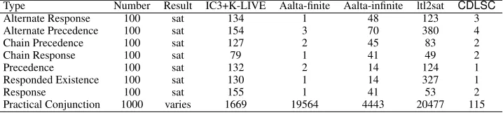
Table 1: Results forLTLfSatisfiability Checking onLT Lf-specific Benchmarks.

spaces:n-bit binary counters for1 ≤ n ≤ 20(Rozier and Vardi 2007). The four templates differ in variables and nest-ing ofX’s.Pattern Formulasencode eight scalable patterns (from (Geldenhuys and Hansen 2006), and are generated by code from (Rozier and Vardi 2007)) scaling ton = 100.

Other LTL formulasthat were used as specifications in re-alistic case studies: (Bloem et al. 2007; De Wulf et al. 2008; Filiot, Jin, and Raskin 2009).

LT Lf-Specific benchmarks consist of the following. Conjunctive Formulascombine commonLT Lf formulas

from (De Giacomo, Masellis, and Montali 2014; Ciccio and Mecella 2015; Prescher, Di Ciccio, and Mendling 2014) as random conjunctions in the style of (Li et al. 2013) in two sets of 500 formulas: (1) 20 variables, varying the number of conjuncts in{10,30,50,70,100}; and (2) 50 conjuncts, varying the number of variables in {10,30,50,70,100}.

Pattern Formulasscalable patterns inspired by (Di Ciccio, Maggi, and Mendling 2016) up to length 100; see Table 1.

Experimental Setup We implement CDLSC in the tool aaltaf2 _{and use Minisat 2.2.0 (E´en and S¨orensson 2003)}

as the SAT engine. We compare it with two extant LTLf

satisfiability solvers: Aalta-finite (Li et al. 2014) and ltl2sat (Fionda and Greco 2016). We also compared with the state-of-art LTL solver Aalta-infinite (Li et al. 2015), using the

LTLf-to-LTL satisfiability-preserving reduction described

in (De Giacomo and Vardi 2013). As LTL satisfiability checking is reducible to model checking, as described in (Rozier and Vardi 2007), we also compared with this reduc-tion, using nuXmv with the IC3+K-LIVE back-end (Cavada et al. 2014), as anLTLf satisfiability checker.

We ran the experiments on a RedHat 6.0 cluster with 2304 processor cores in 192 nodes (12 processor cores per node), running at 2.83 GHz with 48GB of RAM per node. Each tool executed on a dedicated node with a timeout of 60 sec-onds, measuring execution time with Unixtime. Excluding timeouts, all solvers found correct verdicts for all formulas. All artifacts are available in the supplemental material.

Results Figure 2 shows the results for LTLf

satisfiabil-ity checking on LTL-as-LTLf benchmarks.CDLSC

outper-forms all other approaches. On average,CDLSCperforms about 4 times faster than the second-best approach IC3+K-LIVE (1705 seconds vs. 6075 seconds).CDLSCchecks the

LTLfformula directly, while IC3+K-LIVE must take the

in-put of the LTL formula translated from theLTLf formula.

As a result, IC3-KLIVE may take extra cost, e.g., finding a satisfying lasso for the model, to the satisfiability checking.

2

https://github.com/lijwen2748/aaltaf

Meanwhile, CDLSCcan benefit from the heuristics dedi-cated forLTLfthat are proposed in (Li et al. 2014). Finally,

the performance of ltl2sat is highly tied to its performance for unsatisfiability checking as most of the timeout cases for ltl2sat are unsatisfiable. For Aalta-finite, its performance is restricted by the heavy cost of the Tableau Construction.

Table 1 shows the results forLTLf-specific experiments.

Columns 1-3 show the types ofLTLf formulas under test,

the number of test instances for each formula type, and the results by formula type. Columns 4-8 show the check-ing times by formula types in seconds. The dedicatedLTLf

solvers perform extremely fast on the seven scalable pattern formulas (Column 5 and 8), because their heuristics work well on these patterns. For the difficult conjunctive bench-marks,CDLSCstill outperforms all other solvers.

Discussion and Concluding Remarks

There are two ways to apply Bounded Model Checking (BMC) to LTLf satisfiability checking. The first one is to

check the satisfiability of the LTL formula from the input

LTLf formula. Since (Li et al. 2015) showed this approach

performs worse than IC3+K-LIVE,CDLSCoutperforming IC3+K-LIVE implies thatCDLSCalso outperforms BMC. The second approach is to check the satisfiability of the

LTLf formula φdirectly, by unrolling φiteratively. In the

worst case, BMC can terminate (with UNSAT) once the it-eration reaches the upper bound. This is exactly what is im-plemented in ltl2sat (Fionda and Greco 2016).

Our experiments demonstrate that CDLSCoutperforms Aalta-infinite and IC3+K-LIVE, which are designed for LTL satisfiability checking, showing the advantage of a dedicated algorithm for LTLf. Notably,CDLSCmaintains a conflict

(8)

References

Bacchus, F., and Kabanza, F. 1998. Planning for temporally extended goals. Ann. of Mathematics and Artificial Intelli-gence22:5–27.

Bacchus, F., and Kabanza, F. 2000. Using temporal logic to express search control knowledge for planning. Artificial Intelligence116(1–2):123–191.

Bienvenu, M.; Fritz, C.; and McIlraith, S. 2006. Planning with qualitative temporal preferences. InKR, 134–144. Bienvenu, M.; Fritz, C.; and McIlraith, S. A. 2011. Speci-fying and computing preferred plans. Artificial Intelligence 175(7C8):1308 – 1345.

Biere, A.; Cimatti, A.; Clarke, E.; and Zhu, Y. 1999. Sym-bolic model checking without BDDs. InProc. 5th Int. Conf. on Tools and Algorithms for the Construction and Analysis of Systems, volume 1579 ofLecture Notes in Computer Sci-ence. Springer.

Bloem, R.; Galler, S.; Jobstmann, B.; Piterman, N.; Pnueli, A.; and Weiglhofer, M. 2007. Automatic hardware synthesis from specifications: A case study. InDATE, 1188–1193. Bradley, A. 2011. SAT-based model checking without un-rolling. In Jhala, R., and Schmidt, D., eds., Verification, Model Checking, and Abstract Interpretation, volume 6538 ofLNCS. Springer. 70–87.

Calvanese, D.; De Giacomo, G.; and Vardi, M. 2002. Rea-soning about actions and planning in LTL action theories. InPrinciples of Knowledge Representation and Reasoning, 593–602. Morgan Kaufmann.

Camacho, A.; Baier, J.; Muise, C.; and McIlraith, A. 2017. Bridging the gap between LTL synthesis and automated planning. Technical report, U. Toronto.

Cavada, R.; Cimatti, A.; Dorigatti, M.; Griggio, A.; Mariotti, A.; Micheli, A.; Mover, S.; Roveri, M.; and Tonetta, S. 2014. The NuXMV symbolic model checker. InCAV, 334–342. Ciccio, C. D., and Mecella, M. 2015. On the discovery of declarative control flows for artful processes. ACM Trans. Manage. Inf. Syst.5(4):24:1–24:37.

Claessen, K., and S¨orensson, N. 2012. A liveness checking algorithm that counts. InFMCAD, 52–59. IEEE.

De Giacomo, G., and Vardi, M. 1999. Automata-theoretic approach to planning for temporally extended goals. In Proc. European Conf. on Planning, Lecture Notes in AI 1809, 226–238. Springer.

De Giacomo, G., and Vardi, M. 2013. Linear temporal logic and linear dynamic logic on finite traces. InIJCAI, 2000– 2007. AAAI Press.

De Giacomo, G.; Masellis, R. D.; and Montali, M. 2014. Reasoning on LTL on finite traces: Insensitivity to infinite-ness. InAAAI, 1027–1033.

De Wulf, M.; Doyen, L.; Maquet, N.; and Raskin, J.-F. 2008. Antichains: Alternative algorithms for LTL satisfiability and model-checking. InTACAS, volume 4963 ofLNCS, 63–77. Springer.

Di Ciccio, C.; Maggi, F.; and Mendling, J. 2016. Efficient

discovery of target-branched declare constraints. Inf. Syst. 56(C):258–283.

E´en, N., and S¨orensson, N. 2003. An extensible SAT-solver. InSAT, 502–518.

Een, N.; Mishchenko, A.; and Brayton, R. 2011. Efficient implementation of property directed reachability. In FM-CAD, 125–134.

Filiot, E.; Jin, N.; and Raskin, J.-F. 2009. An antichain algorithm for LTL realizability. InCAV, 263–277.

Fionda, V., and Greco, G. 2016. The complexity of LTL on finite traces: Hard and easy fragments. InAAAI, 971–977. AAAI Press.

Gabaldon, A. 2004. Precondition control and the progres-sion algorithm. InKR, 634–643. AAAI Press.

Geldenhuys, J., and Hansen, H. 2006. Larger automata and less work for LTL model checking. InSPIN, volume 3925 ofLNCS, 53–70. Springer.

Gerth, R.; Peled, D.; Vardi, M.; and Wolper, P. 1995. Simple on-the-fly automatic verification of linear temporal logic. In Dembiski, P., and Sredniawa, M., eds.,Protocol Specifica-tion, Testing, and VerificaSpecifica-tion, 3–18. Chapman & Hall. Li, J.; Zhang, L.; Pu, G.; Vardi, M.; and He, J. 2013. LTL satisfibility checking revisited. InTIME, 91–98.

Li, J.; Zhang, L.; Pu, G.; Vardi, M. Y.; and He, J. 2014. LTLf

satisfibility checking. InECAI, 91–98.

Li, J.; Zhu, S.; Pu, G.; and Vardi, M. 2015. SAT-based explicit LTL reasoning. InHVC, 209–224. Springer. Malik, S., and Zhang, L. 2009. Boolean satisfiability from theoretical hardness to practical success. Commun. ACM 52(8):76–82.

Patrizi, F.; Lipoveztky, N.; De Giacomo, G.; and Geffner, H. 2011. Computing infinite plans for LTL goals using a classical planner. InIJCAI, 2003–2008. AAAI Press. Pnueli, A. 1977. The temporal logic of programs. InIEEE FOCS, 46–57.

Prescher, J.; Di Ciccio, C.; and Mendling, J. 2014. From declarative processes to imperative models. SIMPDA 1293:162–173.

Rozier, K., and Vardi, M. 2007. LTL satisfiability checking. InSPIN, volume 4595 ofLNCS, 149–167. Springer. Rozier, K., and Vardi, M. 2010. LTL satisfiability checking. STTT12(2):123–137.

Rozier, K., and Vardi, M. 2011. A multi-encoding approach for LTL symbolic satisfiability checking. InInt’l Symp. on Formal Methods, volume 6664 ofLNCS, 417–431. Springer. Sohrabi, S.; Baier, J. A.; and McIlraith, S. A. 2011. Preferred explanations: Theory and generation via planning. InAAAI, 261–267.

Vardi, M. 2007. Automata-theoretic model checking revis-ited. InVMCAI, LNCS 4349, 137–150. Springer.