The Thirty-Third AAAI Conference on Artificial Intelligence (AAAI-19)
LENA: Locality-Expanded Neural Embedding for Knowledge Base Completion
Fanshuang Kong,
1,2Richong Zhang,
∗1,2Yongyi Mao,
3Ting Deng
1,21SKLSDE, School of Computer Science and Engineering, Beihang University, Beijing, China 2Beijing Advanced Institution on Big Data and Brain Computing, Beihang University, Beijing, China
3School of Electrical Engineering and Computer Science, University of Ottawa, Ottawa, Canada kongfs,zhangrc,[email protected], [email protected]
Abstract
Embedding based models for knowledge base completion have demonstrated great successes and attracted significant research interest. In this work, we observe that existing em-bedding models all have their loss functions decomposed into atomic loss functions, each on a triple or an postulated edge in the knowledge graph. Such an approach essentially implies that conditioned on the embeddings of the triple, whether the triple is factual is independent of the structure of the knowl-edge graph. Although arguably the embeddings of the entities and relation in the triple contain certain structural information of the knowledge base, we believe that the global information contained in the embeddings of the triple can be insufficient and such an assumption is overly optimistic in heterogeneous knowledge bases. Motivated by this understanding, in this work we propose a new embedding model in which we dis-card the assumption that the embeddings of the entities and relation in a triple is a sufficient statistic for the triple’s factual existence. More specifically, the proposed model assumes that whether a triple is factual depends not only on the embedding of the triple but also on the embeddings of the entities and rela-tions in a larger graph neighbourhood. In this model, attention mechanisms are constructed to select the relevant information in the graph neighbourhood so that irrelevant signals in the neighbourhood are suppressed. Termed locality-expanded neu-ral embedding with attention (LENA), this model is tested on four standard datasets and compared with several state-of-the-art models for knowledge base completion. Extensive experiments suggest that LENA outperforms the existing mod-els in virtually every metric.
Introduction
Knowledge bases, such as YAGO, DBpedia and Freebase, have seen explosive growth in many application domains. As most of knowledge bases are extracted from human-edited knowledge sources, the data integrity therein is hardly guar-anteed and the information contained in the knowledge bases is expected to be far from complete. This makesknowledge base completiona particularly important task.
The data in a knowledge base is usually represented as a set of triples, each in the form of(h, r, t), wherehand
tareentitiesandrindicates arelation. The triple(h, r, t)
∗
Corresponding author:[email protected] Copyright c2019, Association for the Advancement of Artificial Intelligence (www.aaai.org). All rights reserved.
in a knowledge base is meant to indicate the fact that h
andtparticipates in the relationr. For example, the triple (Paris, isCapitalOf, France) indicates the fact that Paris is the capital of France. The cross linkage of the factual triples in a knowledge base allows it to be interpreted as a graph where vertices represent entities, edges represent triples, and edge labels represent relations. Since many factual triples are expected missing from a knowledge bases, the objective of knowledge base completion is to discover the missing triples, or edges.
Among the diverse studies in knowledge base com-pletion, knowledge base embedding (Bordes et al. 2013; Wang et al. 2014; Lin et al. 2015; Lin, Liu, and Sun 2015; Dettmers et al. 2018) has demonstrated great successes and is receiving increasing attention at present. Overall this em-bedding methodology falls in the connectionist paradigm of artificial intelligence, in which knowledge base completion is formulated as learning a distributed representation (Hinton, McClelland, and Rumelhart 1986) for entities and relations. With this methodology, the entities and relations in the knowl-edge base are represented as quantities (such as vectors or matrices) in a low-dimensional vector space, and these quanti-ties are learned by minimizing certain loss functions carefully designed to hopefully capture the structure of the knowledge base.
Despite the successes of the embedding models for knowl-edge base completion, this work is motivated by the following observation. In all existing embedding models, the global loss functions decomposes into “atomic” losses, each on a triple
(h, r, t). Although the parameters of the model, or the em-beddings, are linked via the connectivity of the knowledge base, a fundamental assumption in such an approach is that the embeddings for entities, say forhandt, and for relation, say forr, are sufficient to aggregate all structural information contained in the knowledge base for predicting whether the triple(h, r, t)is factual.
Rebecca
Jerry Female
U.S. Berkeley
Gender Nationality Wife
Born in
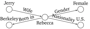
Figure 1: A subgraph of Rebecca.
For example, the embeddings of the “less connected” or “in-frequent” entities and relations may not aggregate sufficient information from learning. Then the assumption that the em-beddings of a triple form a sufficient statistics for predicting its factual existence is expected to fail.
Motivated by this understanding, we relax this assump-tion and take an alternative route from the convenassump-tional ap-proaches. More specifically, we propose a model in which the factual existence of a triple not only depends on the em-beddings of the triple but also depends on the emem-beddings of a larger graph neighbourhood. That is, we expand the “mod-elling locality” from edges to larger graph neighbourhoods. To see that graph neighbourhood information can indeed be helpful, consider the toy example in Figure 1. In the figure, the fact “Rebecca is the wife of Jerry” will be relevant for predicting “Rebecca’s gender is female”, and the fact “Re-becca was born in Berkeley” can be useful for predicting “the nationality of Rebecca is U.S.”. In this example, it is also re-markable that not all information in a given neighbourhood of a triple is relevant to the existence of the triple. To account for such a phenomenon, an attention mechanism is built in our model to (soft-)select the relevant information in a designated graph neighbourhood and suppress the irrelevant noise.
Our proposed model, termed Locality-Expanded Neural Embedding With Attention, or LENA, is tested on four stan-dard datasets and compared against various state-of-the-art models. Experimental results confirm its effectiveness.
Problem Statement and Prior Art
We consider a knowledge Base (KB) as an edge-labelleddirectedgraph, where vertices represent entities, edge labels represent relations, and each directed edge represents a triple
(h, r, t)in the KB. The edge(h, r, t)is labelled byrand has direction pointing from the head entityhto the tail entityt.
Denote the KB of interest byG. That is,G is set of the all factual triples collected in the KB. Each triple in G is also referred to as apositive example. In practice,Gdoes not include all factual triples, and the objective of KB completion is to fillGwith the missing triples. Equivalently, the problem can be formulated as determining whether an arbitrary triple
(h, r, t) ∈ G/ can be factual. Such a triple will be called a
candidate triplefor the ease of reference.
A dominant approach to KB completion is by KB embed-ding. In KB embedding, the entities and relations are mapped to distributed representations (i.e., “embeddings”) in some Euclidean spaces and the structure of the KB is modelled in a loss function relating theses embeddings. Usually the loss function decomposes into the sum of some “atomic” loss function, each involving a positive example, or, if available, a
negative example. The learning of the embeddings is then car-ried out by minimizing the loss function over the embeddings, usually via stochastic gradient descent (SGD). After the em-beddings are obtained, whether a candidate triple is factual can be determined by evaluating the atomic loss function applied to the embeddings of the triple.
Existing Embedding Models
An influential work in KB embedding, TransE (Bordes et al. 2013) uses an atomic loss function that penalizes the dissatisfaction of equaionh+r=t, whereh,randtare the embedding vectors for the head, relation, and tail in a factual triple(h, r, t). The model is later extended to other models, such as TransH(Wang et al. 2014) and TransR(Lin et al. 2015), to better handle one-to-many and many-to-many relations.
The current state-of-the-art embedding models include, to the best of our knowledge, ProjE (Shi and Weninger 2017), DistMult (Yang et al. 2014), Ensemble DistMult (Kadlec, Ba-jgar, and Kleindienst 2017), ComplEx (Trouillon et al. 2016), Analogy (Liu, Wu, and Yang 2017) and ConvE (Dettmers et al. 2018). These models also define their atomic loss func-tions at the triple level. Recently another state-of-the-art em-bedding model R-GCN(Schlichtkrull et al. 2017) has also been presented. Unlike most other models, the successive application of graph convolution(Kipf and Welling 2016) in R-GCN allows the model to pool information beyond the triple level. There are a variety of other embedding mod-els, including, e.g., RESCAL (Nickel, Tresp, and Kriegel 2011), LFM (Jenatton et al. 2012), SME (Bordes et al. 2014), PTransE (Lin, Liu, and Sun 2015), CVSM (Neelakantan, Roth, and McCallum 2015), and a series of models based on graph embedding(Cai, Zheng, and Chang 2017). Also re-lated to this work are some (non-embedding) models for KB completion that exploit graph neighbourhood information. They include, e.g., (Feng et al. ) and (Nguyen et al. 2016) and (Niepert 2016). Except for the Gaifman model (Niepert 2016), most of these models significantly underperform the current art.
LENA
As noted in the previous section, in most KB embedding models, particularly the current state of the art, the “atomic” loss function is defined at the triple level. That is, the loss of a triple(h, r, t), factual or not, depends only on (the em-beddings of) the entities (handr) and relationrinvolved in the triple. In other words, these models assume that the embeddings ofh,randtcontain sufficient information as to whether(h, r, t)is a factual triple. Translated to a proba-bilistic language, such an assumption essentially asserts that
conditioned on the embeddings of(h, r, t)in the KB, whether a triple(h, r, t)could be factual is independent of the KB (graph) structure.
a good amount of structural information has been extracted in the embeddings, there is no convincing reason to believe that the embeddings of some arbitraryh,randtare indeed suffi-cient statistics for the factual existence of the triple(h, r, t). In particular, the heterogeneity of the KB usually would im-ply that the information captured by the embedding of an entity or relation can vary significantly across the KB.
This motivates us to develop an alternative modelling strat-egy in which the “atomic” unit of modelling expands beyond a single edge. More specifically, our fundamental hypothesis is that whether some triple(h, r, t)is factual not only de-pends on the embeddings ofh,randt, but also depends on the embeddings of neighbouring edges (i.e., the adjacent en-tities and relations) in the KB. The model we propose in this paper is termed “locality-expanded neural embedding with attention”, or LENA, since the “locality” of modelling is ex-panded from the edge level to a larger graph neighbourhood and an attention mechanism (Bahdanau, Cho, and Bengio 2015) is also used to (soft) select the relevant information contained in the neighbourhood. We now present LENA.
Setup
We denote by Rthe set of all relations and byN the set of all entities. For reasons that will be come clear later, for each relationr ∈ R, we introduce its reciprocal relation
r−. More precisely, whenever there is a triple(h, r, t), the triple can also be written as(t, r−, h). For example, (Paris, isCapitalOf, France) can be written alternatively as (France, hasCapitalCity, Paris); then isCapitalOf and hasCapitalCIty are a pair of reciprocal relations.
We expand the set Rof relations to the set R˜, which includes the reciprocal relations. That is,R˜ :=R ∪ {r− :
r∈ R}. For each triple(h, r, t)in the KB, we also include its reciprocal triple(t, r−, h)inG. Then whenGis interpreted as a edge-labelled directed graph, every triple(h, r, t)in the KB is represented by two edges: one as an edge with label
rpointing from vertexhto vertext, the other as an edge with labelr−pointing fromttoh. Then the graphGcontains twice as many edges as the number of the triples in the KB. For any given edgee ∈ G , we may useh(e)andt(e)to denote its head and tail entities and user(e)to denote its relation.
Probabilistic Modelling
At the highest level, LENA adopts the probabilistic mod-elling methodology. For any given entityh∈ N and relation
r ∈ R˜, we aim to model the probability that an arbitrary entitytforms a factual triple(h, r, t)withhandr. This prob-ability, denoted byp(t|h, r), is naturally assumed to take the common soft-max form:
p(t|h, r) = Pexp(s(h, r, t))
t0∈N
exp(s(h, r, t0)). (1)
In this model,s(·,·,·)is a scoring function onN ×R ט N, which we will define momentarily. We note that in this formulation, it may appear that we are only concerned with the “tail-prediction” problem(h, r,?). But noting we have
included reciprocal triples and reciprocal relations, any “head-prediction” problem (?, r, t) can be converted to the tail-prediction problem(t, r−,?). Thus this formulation entails
no loss of generality.
Embedding Entities and Relations
We embed entities and relations both as vectors inRk. More specifically, we use a k× |N |matrix DE and a k× |R|˜
matrixDRto represent an entity and a relation respectively:
taking an entityx ∈ N as a one-hot vector inR|N | and a relationr∈R˜as a one-hot vector inR|R|˜, their respective
embedding vectorsxandrcan be expressed as
x := DEx (2)
r := DRr (3)
Note that we used bold font letters to denote the embedding vector of the corresponding entity or relation, and in the rest of the paper, we will continue with this notational convention.
h t
a b c d
r r1
r2 r3
r4 h t
a b c d
r r1
r2 r3
r4
r−
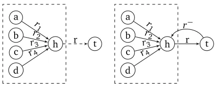
Figure 2: Example of neighbourhood graphsG(h, r, t)(the subgraphs in the dashed boxes) of triple(h, r, t). Triples in
Gare represented by a solid edge, and triples (e.g., candidate triples) not inGare represented by a dashed edge.
Score Function
LetCEandCRbe twok×kmatrices and letbEandbRbe
two vectors inRk. For an arbitrary triple(h, r, t), the score
functions(h, r, t)is parametrized by(CE, CR, bE, bR)and
is defined by
s(h, r, t) :=hvE(h, r, t) +r+bE, CEti
+hvR(h, r, t) +h+bR, CRti,
(4)
wherevE(h, r, t)andvR(h, r, t)are vectors in
Rkand are to
be calculated from the neighbourhood of(h, r, t)in graphG. We note that the introduction of terms vE(h, r, t) and
vR(h, r, t) to the score function is a leap of modelling
methodology in this work. As we will give the construc-tion ofvE(h, r, t)andvR(h, r, t)momentarily, it is precisely due to these terms that the locality is extended beyond the edge level.
As it will become evident, including vE(h, r, t) and
vR(h, r, t)in the score function essentially discards the con-ventional assumption that the factual existence of a triple
Extracting Neighbourhood Information
We now proceed to definevEandvRabove, which are
de-signed to transport information from a larger graph neigh-bourhood.
Neighbourhood For any given triple(h, r, t), we define
G(h, r, t)as
G(h, r, t) :={e∈ G:t(e) =h, e6= (t, r−, h)}.
That is,G(h, r, t)is the subgraph ofGcontaining precisely all edges pointing to entityhexcept the reciprocal edge of
(h, r, t). We will refer to G(h, r, t)as the neighbourhood graph of triple (h, r, t). Figure 2 shows two examples of neighbourhood graphs. In the left figure of Figure 2, the triple(h, r, t)is not originally in the KB. In this case, its re-ciprocal triple(t, r−, h)is not created inG, so the neighbour-hood graph of(h, r, t)contains the edges(a, r1, h),(b, r2, h),
(c, r3, h)and(d, r4, h). In the right figure of Figure 2, the
triple(h, r, t)is in the KB and its reciprocal triple(t, r−, h)
is also included inG. However edge(t, r−, h)is not
consid-ered in the neighbourhood graph of(h, r, t), since(t, r−, h)
is introduced artificially. As such, the neighbourhood graph of(h, r, t)is the same as that in the left figure.
We proceed to explain how information can be extracted from the neighbourhoodG(h, r, t). Although it is possible to extract information from a larger neighbourhood, for train-ing complexity and model capacity considerations, further expansion of locality, paying high price, is expected to result in insignificant return or even overfitting.
To extract information from neighbourhood G(h, r, t), our approach is, to a good extent, motivated by a recent success in sequence modelling exploiting convolution and attention(Kalchbrenner, Grefenstette, and Blunsom 2014; Vaswani et al. 2017).
To that end, letLbe a prescribed positve integer. For any triple(h, r, t), letHL(h, r, t)denote the set of all subsets ofLedges in the neighbourhood graphG(h, r, t). Each of such subset is referred to as awindowofG(h, r, t), since it resembles the notion of window in processing sequence data. The valueLis then referred to as thewindow size.
Using these terminologies, the extracted information can be regarded as being generated in two-step: first, attention mechanisms are used to soft-select the relevant information within each window, and then a pooling operation is applied across the information generated from a set of windows. We now describe the detail of this process.
Windowed Attentions LetΓ∈ HL(h, r, t)be an arbitrary window ofG(h, r, t)containingLedges. We will useh(l; Γ)
to denote the head entity of thel-th edge inΓ, and likewise user(l; Γ)to denote the relation label on the edge.
Let αE
Γ := [αEΓ(0), αEΓ(1), . . . , αEΓ(L)]T be a vector in
RL+1in which each elementαEΓ(l)≥0and
L
P
l=0
αE Γ(l) = 1.
That is, αE
Γ is a probability vector. Similarly, let α R
Γ :=
[αRΓ(0), αΓR(1), . . . , αRΓ(L)]T be a probability vector in
RL+1. The vectorsαEΓ andα R
Γ are to serve as two sets of
attention weights, and their components are defined as fol-low.
αEΓ(l) := exphγ
E
r,h(l; Γ)i
PL
j=0exphγrE,h(j; Γ)i
αRΓ(l) :=
exphγR
r,r(l; Γ)i
PL
j=0exphγrR,r(j; Γ)i
, (5)
whereγrEandγrRare parameter vectors inRk. We note that both attention parametersγE
r andγrRare made dependent of the relation r in the triple (h, r, t) (rather than having the attention parameterγEdepending onh). This break of
symmetry is due to our belief that, it is the relationrrather than entityhthat governs the soft-selection of both entities and relations in the neighbourhoodG(h, r, t).
Using these attention weights, the windowΓgenerates the vectorsvE(Γ)andvR(Γ)in
Rkby
vE(Γ) := αEΓ(0)h+
L
X
l=1
αEΓ(l)h(l; Γ)
vR(Γ) := αRΓ(0)r+
L
X
l=1
αRΓ(l)r(l; Γ). (6)
That is,vE(Γ)is the soft-selected information from
em-beddings ofhand the entities inΓ, andvR(Γ)is the
soft-selected information from embeddings ofrand the relations inΓ. We note that comparing with direct summation or non-parametrized weight summation, such attentive combination or soft-selection reduces the possibility of introducing ir-relevant information, i.e., noise, for predicting the factual existence of(h, r, t).
Cross-Window Pooling The empirical success of CNN has suggested that weighted sum over a sliding window combined with pooling over the windows is a powerful means of extracting features. This motivates us to generate
vE(h, r, t)andvR(h, r, t)by pooling across the outputs from
the windows. Ideally we wish to apply a pooling operation onvE(Γ)’s andvR(Γ)’s across all windows ofG(h, r, t). But this entails combinatorial complexity when entityhis con-nected to a large number of other entities. Additionally such a strategy will also result in the number of windows varying significantly with the size ofG(h, r, t), providing difficulty in parallel training of mini-batches.
For this reason, we turn to a strategy which pools across a fixed number of windows. LetH be a prescribed positive integer. LetHeL(h, r, t)be a random subset ofHL(h, r, t) containing preciselyH windows. Then we definevE(h, r, t)
andvR(h, r, t)as
vE(h, r, t) :=max poolingnvE(Γ) : Γ∈HeL(h, r, t)
o
;
vR(h, r, t) :=max poolingnvR(Γ) : Γ∈HeL(h, r, t)
o
. (7)
At this end, the LENA model, namely, the distribution
Loss Function and Training In the above defined LENA model, the conditional distributionp(t|h, r)for an arbitrary triple(h, r, t)is parametrized byDE,DR,CE,CR,bE,bR,
{γE
r :r∈R}˜ , and{γrR:r∈R}˜ . We denote these parame-ters collectively byΘ. The numberH of windows sampled in a neighbourhood graph and the window sizeLare hyper-parameters of the model.
Given the modelp(t|h, r), it is well-known that the learn-ing of parameterΘunder the maximum-likelihood princi-ple reduces to minimizing the cross entropy between the observed empirical distribution and the model predictive dis-tribution. More precisely, for any given pair(h, r)∈ N ×R˜, letT(h, r) :={t∈ N : (h, r, t)∈ G}.That is,T(h, r)is the set of all entities which have been observed as the tail entity in a triple(h, r, t)inG. LetK:={(h, r)∈ N ×R˜ : (h, r, t)∈ Gfor somet∈ N }.
Under the assumption that for every(h, r)∈ K, the set
T(h, r)is obtained by i.i.d. sampling of the model distribu-tionp(t|h, r). The maximum-likelihood estimateΘ∗of the LENA model reduce to the following cross-entropy mini-mizer:Θ∗:= arg min
Θ P
(h,r)∈K P
t∈T(h,r)
(−logp(t|h, r)).
This loss function is however expensive to optimize in practice. This is due to the large number of entities that results in high complexity in computing the soft-max function and updating its related parameters. Motivated by the approach of (Guillaumin et al. ) and (Shi and Weninger 2017), we restrict the support of the distribution to a random subsetNδ(h, r)of
N, whereδis a prescribed number in(0,1), which we refer to as the “retention rate”.
The construction ofNδ(h, r)is as follows. Draw at uni-formly randomδfraction of the entities inN, and denote the set byAδ(h, r). LetNδ(h, r) :=Aδ(h, r)∪ T(h, r).We then restrict the support of distributionp(·|h, r)toNδ(h, r), by modifyingN in Equation (1) toNδ(h, r).
Finally, following (Guillaumin et al. ) and (Shi and Weninger 2017), we modify the optimization problem to:
Θ∗:=arg min
Θ X
(h,r)∈K X
t∈T(h,r)
− 1
|T(h, r)|logp(t|h, r)
.
(8) In LENA, we optimize Equation (8) using mini-batched SGD, where in each epoch, the setNδ(h, r)for each(h, r)is drawn afresh so that the union of different draws ofNδ(h, r) coversT(h, r).
Experiments
Datasets and Setups
FB15K, WN18, FB15K-237 and WN18-RR are the most commonly used dataset for KB link prediction tasks. We conduct empirical studies on these four datasets to evaluate our model for link prediction.
All four datasets represent multi-relational data as triples. FB15K is a subset of FreeBase, a large-scale general-fact KB, and WN18 is a subset of WordNet, in which entities repre-sent word senses and relations describe lexical relationships between two word senses. It has been noted (Dettmers et al. 2018; Kadlec, Bajgar, and Kleindienst 2017) that for FB15K
Table 1: The statistics of datasets used in this study. Datasets entities relations triples(train/test/valid) FB15K 14,951 1,345 483,142 / 59,071 / 50,000 WN18 40,943 18 141,442 / 5,000 / 5,000 FB15K-237 14,541 237 272,115 / 20,466 / 17,535
WN18-RR 40,943 11 86,835 / 3,134 / 3,034
Table 2: The hyper-parameters of LENA. FB15K FB15K-237 WN18 WN18-RR
L 3 3 5 3
H 90 90 90 60
and WN18 dataset, many testing triples are reciprocal to triples in the training set. So FB15K-237 and WN18-RR are proposed by removing those reciprocal triples from FB15K and WN18. The statistics of the datasets are listed as in Ta-ble 1.
For each triple in the training set (resp. testing set), we produce its reciprocal triple and add it to the training set (resp. testing set). As such the link prediction task is formulated as, for each triple(h, r, t)in the testing set, answer the question
(h, r,?)after the model is trained.
For LENA, the values chosen for retention rate δ are
{0.1,0.25,0.5}. OptimizerAdam (Kingma and Ba 2014) with initial learning rate0.01and mini-batch size 200 is run for 30 epochs. Embedding dimension is chosen as 200. Other hyper-parameter settings of LENA are listed in Table 2.
Evaluation Protocol For each model and for each testing triple(h, r, t), we compute the loss of each triple(h, r, x)
under the model wherexranges over all entities in the KB; we rank these losses from low to high, and obtain the rank for
x=tas the rank for testing case(h, r, t). For models other than LENA, similar ranking is performed for head entityh. For LENA, the loss function is taken as−logp(x|h, r). For other models, their respective loss functions are used.
Evaluation Metrics We use the standard metrics Mean rank (MR) (Bordes et al. 2013), top-10 hit (HIT@10, or sim-ply HIT) (Bordes et al. 2013), reciprocal rank (MRR) (Yang et al. 2014) and their corresponding filtered version metrics, FMR, FHIT and FMRR, to evaluate the model performances. Specifically, MR refers to the average rank of all testing cases, HIT@10 is defined as the percentage of the testing triples that have rank value no greater than 10 and this metric is simply referred as HIT in this paper, and MRR is the average of the multiplicative inverse of the rank value for all testing triples.
The filtered version of three metrics is also considered. In the filtered version, ranking for a testing triple (h, r, t)
is carried out by excluding all entitiesxthat form a triple
(h, r, x)in the training set, validation set or testing set (except
x=t). The filtered MR, HIT@10 and MRR are referred to as F-MR, or F-HIT and F-MR respectively.
Experimental Results and Discussion
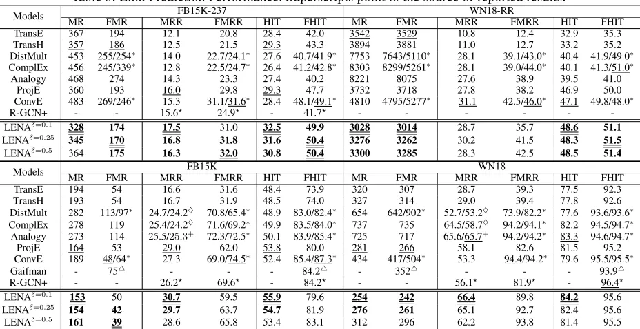
Table 3: Link Prediction Performance. Superscripts point to the source of reported results.
Models FB15K-237 WN18-RR
MR FMR MRR FMRR HIT FHIT MR FMR MRR FMRR HIT FHIT
TransE 367 194 12.1 20.8 28.4 42.0 3542 3529 10.8 12.4 32.9 35.3
TransH 357 186 12.5 21.5 29.3 43.3 3894 3881 11.0 12.7 33.2 35.2
DistMult 453 255/254∗ 14.0 22.7/24.1∗ 27.6 40.7/41.9∗ 7753 7643/5110∗ 28.1 39.1/43.0∗ 40.4 41.9/49.0∗ ComplEx 456 245/339∗ 12.8 22.5/24.7∗ 26.4 41.2/42.8∗ 8303 8299/5261∗ 28.1 39.0/44.0∗ 40.1 41.3/51.0∗
Analogy 468 274 14.3 23.3 27.4 40.2 8221 8075 27.6 38.9 39.5 41.0
ProjE 360 193 16.0 29.8 29.3 47.7 3732 3718 27.8 38.2 46.9 50.0
ConvE 483 269/246∗ 15.3 31.1/31.6∗ 28.4 48.1/49.1∗ 4810 4795/5277∗ 31.1 42.5/46.0∗ 47.1 49.8/48.0∗
R-GCN+ - - 15.6? 24.9? - 41.7? - - - - -
-LENAδ=0.1 328 174 17.5 31.0 32.5 49.9 3028 3014 28.7 35.7 48.6 51.1
LENAδ=0.25 345 170 16.8 31.8 31.6 50.4 3276 3262 30.2 41.5 48.3 51.5
LENAδ=0.5 364 175 16.3 32.0 30.8 50.4 3300 3285 28.3 42.5 48.5 51.4
Models FB15K WN18
MR FMR MRR FMRR HIT FHIT MR FMR MRR FMRR HIT FHIT
TransE 194 54 16.6 31.6 48.4 73.9 320 307 28.7 39.3 77.5 92.3
TransH 193 54 16.7 31.9 48.5 74.0 327 314 29.0 39.4 77.8 92.6
DistMult 282 113/97∗ 24.7/24.2♦ 70.8/65.4∗
48.9 83.0/82.4∗ 654 642/902∗ 52.7/53.2♦ 73.9/82.2∗
77.6 93.6/93.6∗ ComplEx 278 119 25.4/24.2♦ 71.6/69.2∗ 49.9 83.5/84.0∗ 737 735 64.5/58.7♦ 94.2/94.1∗ 82.2 94.5/94.7∗
Analogy 273 114 25.5/25.3+ 72.3/72.5∗
50.1 83.9/85.4∗ 725 717 65.6/65.7+ 94.2/94.2∗
83.3 94.6/94.7∗
ProjE 164 53 29.0 62.0 53.8 80.0 281 266 58.1 82.6 81.5 95.2
ConvE 189 48/64∗ 27.3 69.0/74.5∗ 52.4 85.4/87.3∗ 434 417/504∗ 53.3 94.4/94.2∗ 79.6 95.5/95.5∗
Gaifman - 754 - - - 84.24 - 3524 - - - 93.94
R-GCN+ - - 26.2? 69.6? - 84.2? - - 56.1? 81.9? - 96.4?
LENAδ=0.1 153 50 30.7 59.5 55.9 79.6 254 242 66.4 89.8 84.2 95.6
LENAδ=0.25 154 42 29.7 63.7 54.7 81.9 276 261 65.1 92.7 82.4 95.6
LENAδ=0.5 161 39 28.6 65.8 53.4 83.1 312 296 62.2 93.8 81.4 95.5
TransE and TransH model and use the published code of ProjE model in our experiments.1 For the other compared models, as the performances are not reported on all datasets, we used published code of these models in our experiments in their original parameter settings. For Gaifman and RGCN, we just directly include the reported performance from the original paper.
In Table 3, the values with superscripts are taken from the literature. Specifically, “∗”denotes (Dettmers et al. 2018), “4” denotes (Niepert 2016), “?” denotes (Schlichtkrull et al. 2017), “+” denotes (Liu, Wu, and Yang 2017), and “♦” denotes (Trouillon et al. 2016).
In Table 3, the values without any notation is from our reproduction, the values printed with a single underline are the current “state of the art”. The values printed inboldfont are results of LENA outperforming this “state of the art”. Among them, the top performances are printed in bold font with a double underlines. From the table, it is clear that LENA has the overall best performance. More specifically, on all datasets, LENA (withδ= 0.1,0.25) outperforms any single model in most metrics. For example, on FB15K-237, LENA (δ= 0.25) beats all compared models in all six metrics. On WN18-RR, LENA (δ = 0.25) beats all compared models in five out of six metrics. The only metric on which LENA has not achieved the highest is FMRR. We note however that ConvE has very imbalanced performance: under FMR and FHIT, it underperforms LENA.
1
An author of ProjE has noted the original source code acciden-tally uses testing set in training. We fixed this in our experiments. This leads to degraded performance of ProjE, compared with that in the original paper. For the reimplemented TransE and TransH, we achieve improved performance over the original reported results. Our code is at https://github.com/fskong/LENA.
The performance advantage of LENA on FB15K and WN18 is smaller than that on FB15K-237 and WN18-RR. This is because the testing set of FB15K and WN18 contains a large of fraction of reciprocal triples in the training set. This fact, also noted in (Kadlec, Bajgar, and Kleindienst 2017), offers optimistic artifacts for all models.
It is worth noting that the superior performance of LENA does not come free of cost. Overall the training of LENA takes longer time. For example, when training ProjE and LENA on the same computer, we observe that it takes ProjE 641 seconds to run one epoch, whereas it takes LENA 1524 seconds. For the performance advantage of LENA, we con-sider this additional complexity acceptable.
Behaviour of Attention We now examine the working of the attention mechanism that we build in LENA. For this pur-pose, we compare the prediction performance for each testing triple between LENA and ProjE. The reason that ProjE is chosen for comparison is that when the attention mechanism is disabled, LENA reduces to ProjE2. Thus such a compar-ison allows us to identify how the attention mechanism in LENA functions. To that end, for each testing triple(h, r, t), we define its “rank promotion by LENA” as
rp(h, r, t) :=rankProjE(h, r, t)−rankLENA(h, r, t),
whererankProjE(h, r, t)andrankLENA(h, r, t)are the rank values of(h, r, t)given by ProjE and LENA, respectively.
2
500 1000 1500 2000 2500 3000 3500 4000 4500 5000 0
500 1000
Average Rank Promotion
WN18-RR
500 1000 1500 2000 2500 3000 3500 4000 4500 5000 Entity
0.4 0.5 0.6 0.7 0.8 0.9 1
Weights
0 1 2 3 4 5 7 10 15 Degree
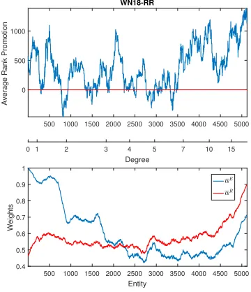
Figure 3:αEandαRvs the degree of entities.
That is,rp(h, r, t)measures by how many positions LENA ranks the testing triple(h, r, t)ahead of ProjE.
For each entitye, letrp(e)be the average ofrp(e, r, t)over all testing triples havingeas the head entity. Also letαE(e)
andαR(e)be respectively the average ofαE(0)and the aver-age ofαR(0)obtained in LENA over all testing triples having
eas the head entity. Note that a higherαE(e)value indicates
that on average predicting triples with head entityeuses less entity information from the neighbourhood graph. Likewise, the corresponding statement can be made forαR(e).
It is possible to obtain the values ofrp(e),αE(e), and
αR(e)for each entityethat has appeared as the head entity in a testing triple. We can sort these entities according to their degrees inGand identify each entityewith its sorted order. Plotting rp(e), αE(e), andαR(e) against the entity order
then allows us to study the behaviour of attention in relation to the entity degrees. Figure 3 is the result of such a study using the WN18RR dataset as an example. In the figure, we have applied a running-window average on the curves with window size 200 to smooth out noisy fluctuations.
On the line between the two plots in Figure 3, the location marked with valuedindicates the location of first window containing an entity having degreed.
In the top figure in Figure 3, the average rank promotion curve is mostly above zero, and often takes high values (a few hundred to a thousand). This correlates well with the overall superior performance of LENA with respect to ProjE. The bottom figure in Figure 3 explains where such rank ad-vantages come from.
For testing triples with low-degree head entities, namely having degree less than3, the rank promotion is primarily due to the relations in the neighbourhood graph (noting that theαRcurve is lower). This can be explained by the fact that for those head entities, there are few entities in the
neighbour-hood graph, therefore the probability that the neighbourneighbour-hood contains helpful entities is very low. However, the probability that the neighbourhood graph contains useful relations can be significantly higher, since WN18RR dataset contains over 40,000 entities but only 18 relations. This significantly higher probability makes the relation information in the neighbour-hood graph play a dominant role in rank promotion.
In the regime where the head entity in the testing triples have degree between 3 and 5, the contribution of the entities in the neighbourhood graph catches up with that of the rela-tions and theαEcurve starts to level and cross theαRcurve.
This can be reasoned by the increased number of entities in the neighbourhood graph and hence increased probability that helpful entities reside therein.
As the degree of the head entities keeps increasing from5, we observe that the neighbouring entities play increasingly stronger roles than the neighbouring relations, and the two curves stay apart. In this regime we also observe that at high degrees, around 7 and above, both curves ramp up, indicating that the contributions from both neighbouring entities and neighbouring relations decay. We speculate that this is due to the following reason. When neighbourhood graph contains more than 7 entities, the number of irrelevant entities and relations it contains also increases and starts to interfere. This challenges LENA’s attention mechanism in detecting signal from noise. When this detection capability decays, the attention mechanism will put more emphasis on the head entity and the relation in the testing triple, relying less on the neighbourhood graph. In degree range, one may also observe that although attention plays weaker roles, the rank promotion is in fact quite high. When carefully looking into the experimental results, we observe that for the test triples in this range, ProjE tends to give poorer rank values (data not shown), and it appears that even weak assistance from the neighbours drastically improves them.
Conclusion
This paper demonstrates that in KB embedding models, the embeddings of a triple(h, r, t)may be insufficient for pre-dicting its factual existence. Extracting and combining in-formation from larger graph neighbourhoods can therefore improve link-prediction performance. We show that atten-tion mechanisms are an effective means of achieving such information extraction and combining. Built on the attention mechanisms, our new model, LENA, has broken a number of performance records, over a range of datasets.
Acknowledgments
This work is supported partly by China 973 program (2015CB358700), by the National Natural Science Foun-dation of China (61772059, 61602023, 61421003), and by the Beijing Advanced Innovation Center for Big Data and Brain Computing and State Key Laboratory of Software De-velopment Environment.
References
Proceedings of the 3rd International Conference on Learning Representations, ICLR.
Bordes, A.; Usunier, N.; Garcia-Duran, A.; Weston, J.; and Yakhnenko, O. 2013. Translating embeddings for modeling multi-relational data. InProceedings of the 27th International Conference on Neural Information Processing Systems, NIPS, 2787–2795.
Bordes, A.; Glorot, X.; Weston, J.; and Bengio, Y. 2014. A semantic matching energy function for learning with multi-relational data.Machine Learning(2):233–259.
Cai, H.; Zheng, V. W.; and Chang, K. C.-C. 2017. A compre-hensive survey of graph embedding: Problems, techniques and applications. arXiv preprint arXiv:1709.07604.
Dettmers, T.; Pasquale, M.; Pontus, S.; and Riedel, S. 2018. Convolutional 2D knowledge graph embeddings. In Proceed-ings of the 32th AAAI Conference on Artificial Intelligence. Feng, J.; Huang, M.; Yang, Y.; and zhu, x. Gake: Graph aware knowledge embedding. InProceedings of the 26th Interna-tional Conference on ComputaInterna-tional Linguistics, COLING, 641–651.
Guillaumin, M.; Mensink, T.; Verbeek, J.; and Schmid, C. Tagprop: Discriminative metric learning in nearest neighbor models for image auto-annotation. InProceedings of the 12th IEEE International Conference on Computer Vision, ICCV, 309–316.
Hinton, G. E.; McClelland, J. L.; and Rumelhart, D. E. 1986. Parallel distributed processing: Explorations in the microstructure of cognition, vol. 1. Cambridge, MA, USA: MIT Press. chapter Distributed Representations, 77–109.
Jenatton, R.; Roux, N. L.; Bordes, A.; and Obozinski, G. 2012. A latent factor model for highly multi-relational data. InProceedings of the 26th International Conference on Neu-ral Information Processing Systems, NIPS, 3167–3175. Kadlec, R.; Bajgar, O.; and Kleindienst, J. 2017. Knowl-edge base completion: Baselines strike back. CoRR
abs/1705.10744.
Kalchbrenner, N.; Grefenstette, E.; and Blunsom, P. 2014. A convolutional neural network for modelling sentences. In
Proceedings of the 52nd Annual Meeting of the Association for Computational Linguistics, ACL, 655–665.
Kingma, D., and Ba, J. 2014. Adam: A method for stochastic optimization. arXiv preprint arXiv:1412.6980.
Kipf, T. N., and Welling, M. 2016. Semi-supervised classification with graph convolutional networks. CoRR
abs/1609.02907.
Lin, Y.; Liu, Z.; Sun, M.; Liu, Y.; and Zhu, X. 2015. Learning entity and relation embeddings for knowledge graph com-pletion. In Proceedings of the 29th AAAI Conference on Artificial Intelligence, 2181–2187.
Lin, Y.; Liu, Z.; and Sun, M. 2015. Modeling relation paths for representation learning of knowledge bases. In
Proceedings of the 2015 Conference on Empirical Methods in Natural Language Processing, EMNLP, 705–714. Liu, H.; Wu, Y.; and Yang, Y. 2017. Analogical inference for multi-relational embeddings. InProceedings of the 34th
International Conference on Machine Learning, ICML, 2168– 2178.
Neelakantan, A.; Roth, B.; and McCallum, A. 2015. Compo-sitional vector space models for knowledge base completion. InProceedings of the Annual Meeting of the Association for Computational Linguistics, ACL, 1–16.
Nguyen, D. Q.; Sirts, K.; Qu, L.; and Johnson, M. 2016. Neighborhood mixture model for knowledge base comple-tion. In Proceedings of the 20th SIGNLL Conference on Computational Natural Language Learning, CoNLL. Nickel, M.; Tresp, V.; and Kriegel, H.-P. 2011. A three-way model for collective learning on multi-relational data. In
Proceedings of the 28th international conference on machine learning, ICML, 809–816.
Niepert, M. 2016. Discriminative gaifman models. In Lee, D. D.; Sugiyama, M.; Luxburg, U. V.; Guyon, I.; and Garnett, R., eds.,Advances in Neural Information Processing Systems 29. Curran Associates, Inc. 3405–3413.
Schlichtkrull, M.; Kipf, T. N.; Bloem, P.; Berg, R. v. d.; Titov, I.; and Welling, M. 2017. Modeling relational data with graph convolutional networks. arXiv preprint arXiv:1703.06103. Shi, B., and Weninger, T. 2017. ProjE: Embedding projection for knowledge graph completion. InProceedings of the 31st AAAI Conference on Artificial Intelligence, 1236–1242.
Trouillon, T.; Welbl, J.; Riedel, S.; Gaussier, ´E.; and Bouchard, G. 2016. Complex embeddings for simple link pre-diction. InProceedings of the 33nd International Conference on Machine Learning, ICML, 2071–2080.
Vaswani, A.; Shazeer, N.; Parmar, N.; Uszkoreit, J.; Jones, L.; Gomez, A. N.; Kaiser, L. u.; and Polosukhin, I. 2017. Attention is all you need. InThe 31st Advances in Neural Information Processing Systems, NIPS, 6000–6010. Wang, Z.; Zhang, J.; Feng, J.; and Chen, Z. 2014. Knowledge graph embedding by translating on hyperplanes. In Proceed-ings of the 28th AAAI Conference on Artificial Intelligence, 1112–1119.