R E V I E W
Open Access
The hyperpycnite problem
G. Shanmugam
Abstract
Sedimentologic, oceanographic, and hydraulic engineering publications on hyperpycnal flows claim that (1) river
flows transform into turbidity currents at plunge points near the shoreline, (2) hyperpycnal flows have the power to
erode the seafloor and cause submarine canyons, and, (3) hyperpycnal flows are efficient in transporting sand across
the shelf and can deliver sediments into the deep sea for developing submarine fans. Importantly, these claims do
have economic implications for the petroleum industry for predicting sandy reservoirs in deep-water petroleum
exploration. However, these claims are based strictly on experimental or theoretical basis, without the supporting
empirical data from modern depositional systems. Therefore, the primary purpose of this article is to rigorously evaluate
the merits of these claims.
A global evaluation of density plumes, based on 26 case studies (e.g., Yellow River, Yangtze River, Copper River,
Hugli River (Ganges), Guadalquivir River, Río de la Plata Estuary, Zambezi River, among others), suggests a complex
variability in nature. Real-world examples show that density plumes (1) occur in six different environments (i.e., marine,
lacustrine, estuarine, lagoon, bay, and reef); (2) are composed of six different compositional materials (e.g., siliciclastic,
calciclastic, planktonic, etc.); (3) derive material from 11 different sources (e.g., river flood, tidal estuary, subglacial, etc.);
(4) are subjected to 15 different external controls (e.g., tidal shear fronts, ocean currents, cyclones, tsunamis, etc.); and,
(5) exhibit 24 configurations (e.g., lobate, coalescing, linear, swirly, U-Turn, anastomosing, etc.).
Major problem areas are: (1) There are at least 16 types of hyperpycnal flows (e.g., density flow, underflow, high-density
hyperpycnal plume, high-turbid mass flow, tide-modulated hyperpycnal flow, cyclone-induced hyperpycnal turbidity
current, multi-layer hyperpycnal flows, etc.), without an underpinning principle of fluid dynamics. (2) The basic tenet
that river currents transform into turbidity currents at plunge points near the shoreline is based on an experiment that
used fresh tap water as a standing body. In attempting to understand all density plumes, such an experimental result is
inapplicable to marine waters (sea or ocean) with a higher density due to salt content. (3) Published velocity measurements
from the Yellow River mouth, a classic area, are of tidal currents, not of hyperpycnal flows. Importantly, the presence of tidal
shear front at the Yellow River mouth limits seaward transport of sediments. (4) Despite its popularity, the hyperpycnite
facies model has not been validated by laboratory experiments or by real-world empirical field data from modern settings.
(5) The presence of an erosional surface within a single hyperpycnite depositional unit is antithetical to the basic principles
of stratigraphy. (6) The hypothetical model of
“
extrabasinal turbidites
”
, deposited by river-flood triggered hyperpycnal flows,
is untenable. This is because high-density turbidity currents, which serve as the conceptual basis for the model, have never
been documented in the world
’
s oceans. (7) Although plant remains are considered a criterion for recognizing
hyperpycnites, the
“
Type 1
”
shelf-incising canyons having heads with connection to a major river or estuarine
system could serve as a conduit for transporting plant remains by other processes, such as tidal currents. (8) Genuine
hyperpycnal flows are feeble and muddy by nature, and they are confined to the inner shelf in modern settings.
(9) Distinguishing criteria of ancient hyperpycnites from turbidites or contourites are muddled. (10) After 65 years of
research since Bates (AAPG Bulletin 37: 2119
–
2162, 1953), our understanding of hyperpycnal flows and their deposits is
still incomplete and without clarity.
Keywords:
Density plumes, Facies model, Hyperpycnites, Submarine fans, Tidal shear fronts, Ocean currents, Turbidity
currents, Yellow River, Yangtze River
Correspondence:[email protected]
Department of Earth and Environmental Sciences, The University of Texas at Arlington, Arlington, TX 76019, USA
Journal of Palaeogeography
© The Author(s). 2018Open AccessThis article is distributed under the terms of the Creative Commons Attribution 4.0 International License (http://creativecommons.org/licenses/by/4.0/), which permits unrestricted use, distribution, and reproduction in any medium, provided you give appropriate credit to the original author(s) and the source, provide a link to the Creative Commons license, and indicate if changes were made.
1 Introduction
1.1 The incentive
The term
“
hyperpycnite
”
(i.e., deposits of hyperpycnal
flows) was first introduced by Mulder et al. (
2002
) in an
academic debate with me (Shanmugam
2002
) on the
origin of inverse grading by hyperpycnal flows. The
following year, Mulder et al. (
2003
) published their
review paper with the introduction of the genetic facies
model of hyperpycnites. I have been an ardent critic of
all genetic facies models. Examples are:
1)
“Is the turbidite facies association scheme valid for
interpreting ancient submarine fan environment?”
(Shanmugam et al.
1985
).
2)
“The Bouma sequence and the turbidite mind set”
(Shanmugam
1997
).
3)
“
The tsunamite problem
”
(Shanmugam
2006b
).
4)
“The landslide problem”
(Shanmugam
2015
).
5)
“Submarine fans: A critical retrospective (1950
−
2015)
”
(Shanmugam
2016a
).
6)
“The contourite problem”
(Shanmugam
2016b
).
7)
“The seismite problem”
(Shanmugam
2016c
).
In continuing this trend, it is only logical to contribute
this paper
— “
The hyperpycnite problem
”
.
1.2 The history
Forel (
1885
,
1892
) first reported the phenomenon of
density plumes in the Lake Geneva (Loc Léman),
Switzerland (Fig.
1
). In advocating a rational theory for
delta formation, Bates (
1953
) suggested three types: (1)
hypopycnal plume for floating river water that has lower
density than basin water (Fig.
2a
); (2) homopycnal plume
for mixing river water that has equal density as basin
water (Fig.
2b
); and (3) hyperpycnal plume for sinking
river water that has higher density than basin water (Fig.
2c
). Mulder et al. (
2003
) expanded the applicability of
the concept of hyperpycnal plumes from shallow water
(deltaic) to deep-water (continental slope and abyssal
plain) environments. In this new development,
hyper-pycnal flows are considered analogous to turbidity
cur-rents in many respects (Mulder et al.
2003
; Steel et al.
2016
; Zavala and Arcuri
2016
).
During the past four decades, there has been an
accel-erated effort to understand these density plumes through
(1) observational and/or interpretational (Arnau et al.
2004
; Bhattacharya and MacEachern
2009
; Collins et al.
2017
; Gihm and Hwang
2016
; Johnson et al.
2001
; Lewis
et al.
2018
; Luo et al.
2017
; Milliman et al.
2007
; Mulder
et al.
2003
; Mutti et al.
1996
; Ogston et al.
2000
; Pan
et al.
2017
; Petter and Steel
2006
; Pierce
2012
; Puig et al.
2014
; Schillereff et al.
2014
; Shanmugam
2016a
,
2018a
,
2018b
,
2018c
; Soyinka and Slatt
2008
; Steel et al.
2016
,
2018
; Sun et al.
2016
; Talling
2014
; Warrick et al.
2013
;
Wilson and Schieber
2014
,
2017
; Wright et al.
1986
,
1988
; Yang et al.
2017a
; Zavala and Arcuri
2016
; Zavala
and Pan
2018
; Zavala et al.
2006
; among others), (2)
ex-perimental (Kostic and Parker
2003
; Kostic et al.
2002
;
Lamb and Mohrig
2009
; Lamb et al.
2010
; Parsons et al.
2001
), and (3) numerical (Chen et al.
2013
; Kassem and
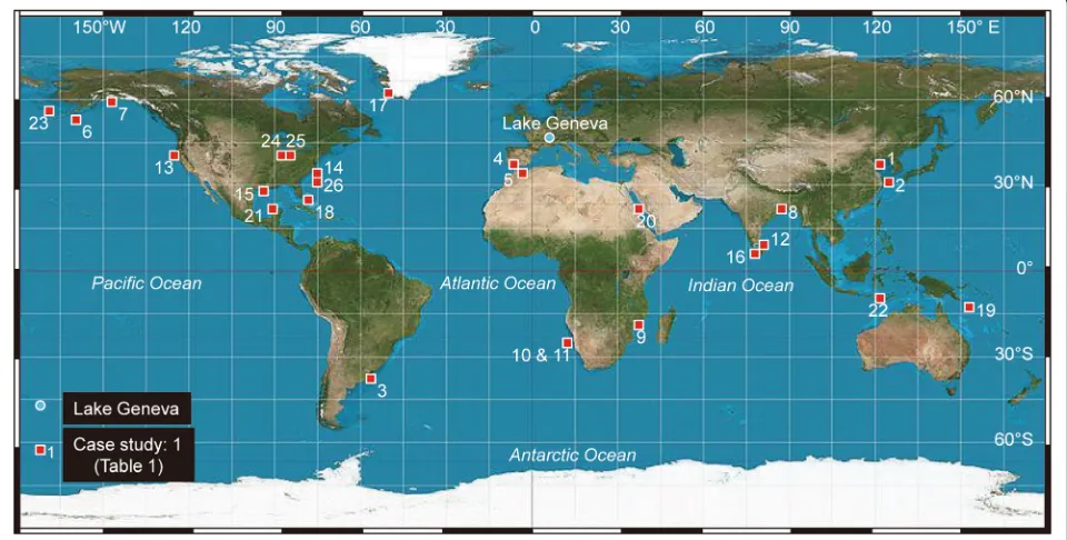
Fig. 1Location map of 26 case studies of marine and lacustrine environments (Table1). Forel (1885,1892) first reported the phenomenon of density
Imran
2001
; Khan et al.
2005
; Kostic and Parker
2003
;
Morales de Luna et al.
2017
; Qiao et al.
2008
; Wang and
Wang
2010
; Wang et al.
2017
; among others) studies.
1.3 The problem
Despite popular claims that (1) river flows transform
into turbidity currents at plunge points near the
shore-line (Kostic et al.
2002
; Lamb et al.
2010
), (2)
hyperpyc-nal flows have the power to erode the seafloor and cause
submarine canyons (Lamb et al.
2010
), (3) hyperpycnal
flows develop an unique vertical sequence (i.e., facies
model) (Mulder et al.
2003
), and, (4) hyperpycnal flows
are efficient in transporting sand across the shelf and
can deliver sediments into the deep sea for developing
submarine fans (Zavala and Arcuri
2016
), our
under-standing of hyperpycnal flows and their deposits, in
par-ticular, in deep-water settings (i.e., seaward of the
shelf-slope break at about 200 m water depth, Fig.
3
), is
highly speculative.
Specific issues are:
1) There is not a single documented case of hyperpycnal
flow, which is transporting sand across the continental
shelf, and supplying sand beyond the modern shelf
break (Fig.
3
).
2) Thus far, the emphasis has been solely on
river-mouth hyperpycnal flows (Mulder et al.
2003
), thus
ignoring density plumes in other environments,
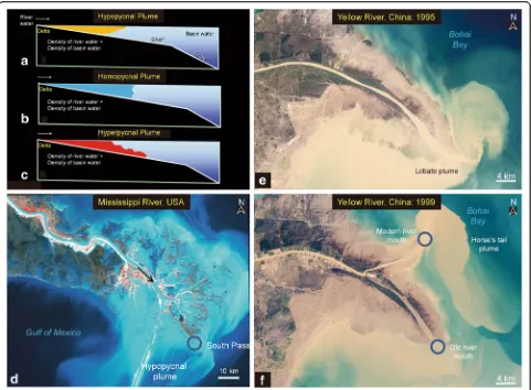
Fig. 2Concepts and examples of density plumes.a,b, andcSchematic diagrams showing three types of density variations in riverine plumes in
deltaic environments based on concepts of Bates (1953).aHypopycnal plume in which density of river water is less than density of basin water; bHomopycnal plume in which density of river water is equal to density of basin water;cHyperpycnal plume in which density of river water is greater than density of basin water. Figure from Shanmugam (2012) with permission from Elsevier Handbook of Petroleum Exploration and Production. License Number: 4259411120776. License Date: December 31, 2017;dImage of the Mississippi River showing well-developed floating hypopycnal plumes. Note“deflecting”plumes. Black arrow shows river course for the South Pass (Walker et al.,1993). Circle shows river mouth. See Coleman and Prior (1982) for river-dominated deltaic facies model. Image credit: NASA;eSatellite image of the Yellow River showing well-developed lobate plume at the old river mouth. Image credit: NASA Earth Observatory. https://earthobservatory.nasa.gov/Features/WorldOfChange/yellow_river.php?all=y; f Satellite image of the Yellow River showing horse’s tail plume at the modern river mouth that was initiated in 1996. Two circles show old and modern river mouths. Image credit: NASA Earth Observatory.https://earthobservatory.nasa.gov/Features/WorldOfChange/yellow_river.php?all=y
such as open marine settings, far away from the
shoreline.
3) Despite their common occurrence, density plumes
triggered by tidal currents, glacial meltwater, eolian
dust, volcanic explosion, cyclones, tsunamis, upwelling,
etc.
are
largely
ignored
from
sedimentological
investigations.
4) Specifically, there are fundamental problems associated
with the concept of hyperpycnal flows in terms of
fluid dynamics, depositional mechanisms, sedimentary
structures, etc., which generated a lively debate
(Mulder et al.
2002
; Shanmugam
2002
).
5) Finally, hyperpycnite facies models have implications
for the petroleum industry for predicting sandy
reservoirs in deep-water petroleum exploration and
exploitation. For example, Yang et al. (
2017a
, p. 115)
in their article published in the
AAPG Bulletin
stated
that
“
The lacustrine hyperpycnites of the Yanchang
Formation have important implications for
uncon-ventional petroleum exploitation
”. Shanmugam
(
2018a
) discussed this study in terms of inherent
problems with data, documentation, and facies
model.
1.4 The objective
In addressing the above listed problems, the primary
pur-pose of this article is to rigorously evaluate the merits of
various claims on hyperpycnal flows and related facies
models. This evaluation is based on 26 case studies (Fig.
1
;
Table
1
). Each case study is used in identifying problem
areas. In particular, the Yellow River in China is used as
the prime example because of its historical significance
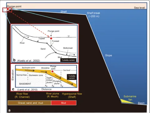
Fig. 3Continental margin and flume experiments.aConceptual diagram of a continetal margin showing relative positions of plunge point (red
Table
1
Config
ura
ti
o
ns
of
d
e
nsit
y
p
lu
me
s
o
n
sa
te
lli
te
ima
g
es
in
mo
de
rn
ma
ri
n
e
an
d
la
cu
str
in
e
e
n
vi
ro
n
m
e
n
ts
.Se
e
Sh
an
m
u
ga
m
(
2
018
b
)
for
a
com
pr
ehensiv
e
st
udy
o
f
4
5
ca
se
studi
es
Serial num ber in Fig. 1 Case st udy an d loc ation Configu ration of de nsity plume s on satellite images Envi ronme nt External contro l Comm ents 11 A − Yellow Riv er, Bohai Bay 1A − Simp le lobate, asso ciated with a sing le river mouth (old river mou th, 1995 ; Fig. 2e ) Riv er-domi nated delta Tidal she ar front (Wan g et al. 2010 ) Interp retat ion of a specific type of plu me in the an cient record is impractical at pre sent. 1B − Yellow Riv er, Boh ai Bay 1B − Horse ’ s tai l (Mode rn rive r mouth, 19 99; Fig. 2f ) Riv er-domi nated delta Tidal she ar front (Wan g et al. 2010 ) Interp retat ion of a specific type of plu me in the an cient record is impractical at pre sent. 2 Yangtze Riv er, East China Sea Deflec ting (Fig. 11a ) Ti de-dom inated es tuary Shelf curre nts (Liu et al. 2006 ) Vertic al mixing by tides in wint er month s (Luo et al. 2017 ) Interp retat ion of a specific type of plu me in the an cient record is impractical at pre sent. 3 Río de la Pla ta Estuary , Argent ina an d Urug uay, South Atlant ic O cean Dissipating (Fig . 20c ) Mar ine Ocean curre nts (Gonz alez-Silve ra et al. 20 06 ; Matano et al. 2010 ) Interp retat ion of a specific type of plu me in the an cient record is impractical at pre sent. 4 Guadalquivir River, Sou thern Spain, Gulf of Cád iz U-Turn (Fig. 22c ) Riv er-domi nated delta Surace and slop e curre nts (Peliz et al. 20 09 ) Interp retat ion of a specific type of plu me in the an cient record is impractical at pre sent. 5 Strait of Gibral tar Swirly (NASA 2017 ) Strai t mou th Ocean water moving throu gh the strait and inte rnal wave s (Shanm ugam 2013 ) Interp retat ion of a specific type of plu me in the an cient record is impractical at pre sent. 6 Chign ik Lak e, Alas ka, Pac ific O cean Linear (Fig. 6 ) Brai ded de lta in a lag oon, Pacific Ocean Coars e-grained braide d de lta (McPhe rson et al. 1987 ) Interp retat ion of a specific type of plu me in the an cient record is impractical at pre sent. 77 A − Copp er River, Gulf of Alas ka 7A − Coale scing irregu lar, associ ated with multiple river mouths (Fig. 24a ) Brai ded de lta, mar ine Coars e-grained braide d de lta Interp retat ion of a specific type of plu me in the an cient record is impractical at pre sent. 7B − Copper River, Gulf of Alas ka 7B − Blanket ing eoli an dust plume (Fig. 24 b ) Brai ded de lta, mar ine Eolian Interp retat ion of a specific type of plu me in the an cient record is impractical at pre sent. 8 Hugli Riv er (a distr ibutary of the Ganges Riv er), India, Bay of Bengal Anastom osing (Fig. 25b ) Ti de-dom inated es tuary (Bala subram anian and Ajm al Khan 20 02 ) Tidal curre nts The Bay of Bengal is known not only for severe mons oona l flo ods, but also for frequ ent cyclonic activ ity (Shanm ugam 2008a ) Interp retat ion of a specific type of plu me in the an cient record is impractical at pre sent. 9 Zambezi River, Central Moz ambique, Indian Ocean Coalescing lobate, asso ciated with multiple river mouths (Fig. 23 ) Wav e-do minated delta Longshore currents (Mikhai lov et al. 2015 ) Interp retat ion of a specific type of plu me in the an cient record is impractical at pre sent. 10 Off Nam ibia, Sou th Atlant ic Cloudy (NAS A 20 17 ) Mar ine Upwel ling (Plankt on) (Shilling ton et al. 1992 ) Interp retat ion of a specific type of plu me in the an cient record is impractical at pre sent. 11 Off Nam ibia, Sou th Atlant ic Swirly (NASA 2017 ) Mar ine Upwel ling (Hyd rogen sulf ide) Interp retat ion of a specific type of plu me in the an cient record is impractical at pre sent. 12 Gulf of Mannar, Indi a an d Sri Lank a, Indian Ocean Massive and swi rly (NASA 2017 ) Mar ine Mons oonal currents (Jagadeesan et al. 20 13 ); wave actions (Sridhar et al. 2008 ) Interp retat ion of a specific type of plu me in the an cient record is impractical at pre sent. 13 Golde n Gat e Bridge, San Fra ncisco Bay, Pacific Ocean Tidal lobate (Fig. 26c ) Bay mou th Tidal curre nts (Barnard et al. 20 06 ) Interp retat ion of a specific type of plu me in the an cient record is impractical at pre sent. 14 U.S. Atlant ic shelf Cascad ing (Shanm uga m 2008a ) She lf (Mari ne) 1999 Hurricane Flo yd a Interp retat ion of a specific type of plu me in the an cient record is impractical at pre sent.(Milliman and Meade
1983
) and its data-rich
environ-ments (Wright et al.
1986
). This paper is organized into
the following topics: (1) basic concepts, (2) the Yellow
River, (3) the Yangtze River, (4) external controls, (5)
rec-ognition of ancient hyperpycnites, (6) submarine fans, (7)
submarine canyons, and (8) configurations of density
plumes. The ultimate goal here is to identify problem
areas and to alert students of challenges in their future
re-search and to identify opportunities for future rere-search.
2 Basic concepts
In this review, which covers multiple disciplines (e.g.,
process sedimentology, physical oceanography,
meteor-ology, hydraulic engineering, etc.), it is necessary to
es-tablish at the outset some basic concepts and related
nomenclatures.
2.1 Hyperpycnite
As mentioned at the outset, the term
“
hyperpycnite
”
was introduced by Mulder et al. (
2002
) in an
aca-demic debate with me (Shanmugam
2002
) on the
ori-gin of inverse grading by hyperpycnal flows. Mulder
et al. (
2002
) attempted to differentiate
“
hyperpycnites
”
deposited by hyperpycnal turbidity currents from
“
classic turbidites
”
deposited from failure-related
tur-bidity currents. The problem is that triggering
mecha-nisms of turbidity currents (or any other process)
cannot be determined from the depositional record
(Shanmugam
2015
,
2016a
,
2016b
,
2016c
).
2.2 Continental margin
A basic conceptual framework is used in which a river
mouth is located near the shoreline, whereas a submarine
fan is located at the base of the continental slope,
sepa-rated by a wide continental shelf (Fig.
3a
). In order for river
plumes to act as hyperpycnal flows and deliver sediment to
the deep sea for developing submarine fans (Zavala and
Arcuri
2016
), hyperpycnal flows must travel 10s to 100s of
kilometers across the shelf from their point of origin.
2.3 Plunge point
The term
“
plunge point
”
is used for both
“
plunging
waves
”
and
“
plunging rivers
”
. According to the
Glossary
of Coastal Terminology
(
1998
), a plunging wave is
de-fined as the point at which the wave curls over and falls.
According to Assireu et al. (
2011
), for plunging rivers,
the plunge point is the main mixing point between river
and epilimnetic reservoir. In other words, the point at
which sediment-laden river flow plunges down into a
standing body of water, be it a lake, a reservoir, or a sea.
Plunging occurs very close to the shoreline in shallow
water (Fig.
3b
). In the Yellow River in China, for
ex-ample, the plunge point occurs at 5 m of depth in the
Bohai Bay (Wright et al.
1986
). When a river flow
crosses the plunge point at the river mouth, it
trans-forms into a river plume of various densities, which
in-clude hyperpycnal plumes (Fig.
2c
). At the plunge point,
the river flow moves from a momentum-dominated type
to a buoyancy-dominated type and marks the transition
of an inflow to an underflow (Dallimore et al.
2004
).
At the plunge point, the river has already dropped its
coarse
fractions
(gravel
and
sand)
upstream
as
delta-plain facies. The remaining fine fractions in muddy
suspension move forward on the open shelf as
hyperpyc-nal flows. Plunging would occur only if suspended
sedi-ment concentration in the river exceeds the critical
value of 35
−
45 kg·m
−3(Imran and Syvitski
2000
; see
Mulder et al.
2003
for differences in values between
equatorial and subpolar rivers).
2.4 Plume versus flow
In practice, there is a tendency to equate the term
“
flow
”
with
“
plume
”
. These two terms are not one and not the
same. In hydrodynamics, the term plume describes a
condition when a column of one fluid moves through
another fluid. To accommodate natural variability in
plume types, a broad definition of plume is adopted in
this article. Accordingly, a plume is a fluid enriched in
sediment, ash, biological or chemical matter that enters
another fluid. As it would be demonstrated later, there is
a multitude of plume types in nature. Among them, the
river plume is the most popular. NOAA Fisheries
Gloss-ary (
2006
, p. 42) defines a
River Plume
as
“Turbid
fresh-water flowing from land and generally in the distal part
of a river (mouth) outside the bounds of an estuary or
river channel”
.
However, the term
“
flow
”
is used for a continuous,
ir-reversible deformation of sediment-water mixture that
occurs in response to applied shear stress, which is
grav-ity in most cases (Pierson and Costa
1987
, p. 2). Not all
plumes are flows. For example, floating hypopycnal
plumes are not driven by gravity (Fig.
2a
). However, both
terms
“
flow
”
and
“
plume
”
are applicable to hypepycnal
type. The other practice is to employ terms
“
overflow
”
,
“
interflow
”
, and
“
underflow
”
for hypopycnal,
homopyc-nal, and hyperpycnal plumes, respectively. Again, the
term flow is not appropriate for hypopycnal plume that
is unaffected by gravity.
2.5 Types of river-mouth flows
In discussing river-mouth processes, geologists,
geophys-icists, and hydraulic engineers use process terms to
rep-resent hyperpycnal flows that are not consistent in
meaning with each other, such as single-layer and
multi-layer hyperpycnal flows (Fig.
4
; see Section
3.5
).
For example, the following concepts and terms are used
in the literature:
1) Density flow (Parker and Toniolo
2007
).
2) Underflow (Wright et al.
1986
).
3) Hyperpycnal flow (Bates
1953
; Moore
1966
).
4) Hyperpycnal underflow (Wright et al.
1986
).
5) Hyperconcentrated flow (van Maren et al.
2009
).
6) Low-density hyperpycnal plume (Wright et al.
1986
).
7) High-density hyperpycnal plume (Wright et al.
1986
).
8) High-turbid mass flow (Fan et al.
2006
).
9) Supercritical hyperpycnal flow (Yang et al.
2017b
).
10) Tide-modulated
hyperpycnal
flow
(Fig.
4d
)
(Wang et al.
2010
).
11) Cyclone-induced hyperpycnal turbidity current
(Liu et al.
2012
).
12) Buoyancy-dominated flow (Dallimore et al.
2004
).
13) Hyperpycnal turbidity current (Plink-Björklund and
Steel
2004
).
14) Turbidity front (Frami
ň
an and Brown
1996
).
15) Turbidity current (Kostic and Parker
2003
; Kostic
et al.
2002
; Lamb et al.
2010
; Wright et al.
1986
;
Zavala and Arcuri
2016
).
16) Multi-layer hyperpycnal flows (Morales de Luna
et al.
2017
).
These 16 river-mouth processes, some with
superflu-ous meanings, do not have a unifying principle of fluid
dynamics as their foundation. It is confusing when
geologists manufacture a plethora of superfluous names
for a single process. In this tradition, the concept of
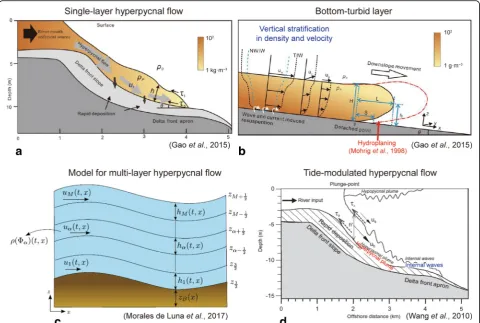
Fig. 4 Variable types of hyperpycnal flows.a Single-layer hyperpycnal flow, Yellow River, China. Color concentration = Suspended sediment
concentration; h = Flow thickness;τt= Upper surface;τb= Bed shear stress. From Gao et al. (2015);bBottom turbid layer with density and velocity
stratification (i.e., debris flow with hydroplaning, red arrow added in this article, see text), Yellow River, China. Uw= Wave orbital velocity; Uc= Along
shelf current magnitude; Ug= Velocity of gravity current; NWIW = Normal wind-induced wave velocity; TIW = Typhoon-induced wave. The red line
“
high-density turbidity currents
”
is the leader with 34
synonymous terms (Shanmugam
2006a
).
2.6 River currents versus turbidity currents
The practice of equating subaqueous turbidity currents
with subaerial river currents (Chikita
1989
) is confusing
for many reasons (Table
2
). River currents and turbidity
currents are fundamentally different, although both are
turbulent in state (Middleton
1993
). River currents are
low in suspended sediment (1%
−
5% by volume; Galay
1987
), whereas turbidity currents (i.e., low-density
tur-bidity currents) are relatively high in suspended
sedi-ment (1%
−
23% by volume; Middleton
1993
), although
both currents are considered to be Newtonian in
rhe-ology (Table
2
). River currents are fluid-gravity flows,
whereas turbidity currents are sediment-gravity flows
(Middleton
1993
), which is the most important
distinc-tion. To reiterate, a turbidity current is a sediment flow
with Newtonian theology and turbulent state in which
sediment is supported by fluid turbulence and from
which deposition occurs through suspension settling
(Dott
1963
; Middleton and Hampton
1973
; Sanders
1965
; Shanmugam
1996
,
2006a
; Talling et al.
2012
). In
addition, according to Bagnold (
1962
), typical turbidity
currents can function as truly turbulent suspensions
only when their sediment concentration by volume is
below 9%. Therefore, river currents should not be
equated with turbidity currents.
In the 1930s, density currents (Daly
1936
) and turbidity
currents were considered to be one and the same. Since
then, the domain of turbidity currents went through a
re-markable period of revolution and evolution (Shanmugam
2016a
). After 80 years of research, we have come full
circle. Today, we once again consider density currents and
turbidity currents to be one and the same. For example,
Parker and Toniolo (
2007
, p. 690) defined a turbidity
current as follows:
“When the density difference is
medi-ated by the presence of suspended mud in the water
column of the river, the resulting underflow is termed a
turbidity current”
. However, the distinction is that all
tur-bidity currents are density currents, but not all density
currents are turbidity currents (e.g., thermohaline-density
driven bottom currents or
“
contour currents
”
(Hollister
1967
)). It should be reiterated that all hyperpycnal plumes
are density plumes, but not all density plumes are
hyper-pycnal plumes (e.g., hypohyper-pycnal and homohyper-pycnal plumes).
This confusion can be easily avoided by simply adhering
to the established concepts available in sedimentologic
lit-erature (Bagnold
1962
; Dott
1963
; Middleton and
Hampton
1973
; Sanders
1965
; Shanmugam
1996
,
2006a
,
2018c
; Talling et al.
2012
).
The first step in evaluating density plumes is to
distin-guish a
“
plume
”
from a
“
flow
”
and to differentiate a
“
river current
”
from a
“
turbidity current
”
.
2.7 Transformation of river currents into turbidity
currents
Based on experimental (Kostic et al.
2002
) and
numer-ical simulation, Kostic and Parker (
2003
) suggested that
river currents transform into turbidity currents at the
plunge point (Fig.
3b
). Because Kostic et al. (
2002
) used
fresh water in their experiment as a standing body of
water, care must be exercised in applying the
experimen-tal results (i.e., initiation of turbidity currents at the
plunge point) to marine settings (sea or ocean), which is
the focus of this article. There are concerns with the
ex-perimental/numerical model.
1) Average density of sea water at the surface is
1.025 kg·L
−1, whereas that of fresh water is 1.0
kg·L
−1at 4 °C (39 °F). This density difference is
crucial for understanding the generation of a
density flow, such as the hyperpycnal flow.
2) No one has documented the transformation of river
currents into turbidity currents at a shallow plunge
point in modern marine environments.
3) These river-flow triggered turbidity currents in
laboratory experiments, yet to be documented in
modern
marine
settings,
are
muddy
flows.
Therefore, they are of no consequence in transporting
sand and gravel across the continental shelf and deliver
the sediment into the deep sea for developing
submarine fans.
4) Importantly, not all density flows are turbidity
currents. For example, although both debris flows
and turbidity currents are considered to be density
flows, each one can be distinguished from the other
by fluid rheology and flow turbulence (Dott
1963
;
Sanders
1965
). Such a distinction is not considered
in defining hyperpycnal flows. Hyperpycnal flows
are defined solely on the basis of fluid density.
Therefore, it is misleading to equate turbidity
Table 2
Comparison of subaerial river currents and subaqueous
turbidity currents (partly based on Shanmugam
1997)
Features River currents Turbidity currents
Ambient fluid Air Water
Rheology of fluid Newtonian Newtonian
Type of gravity influence
Fluid gravity Sediment gravity
Nature of flow Uniform\steady\ and continuous
Uniform\unsteady\ and episodic
Sediment concentration
Low (1%−5% by volume)
High (1%−23% by volume)
Dominant transport of sand
Bed load Suspended load
Dominant structures Cross bedding Normally graded bedding
currents with hyperpycnal flows (Kostic et al.
2002
;
Lamb et al.
2010
; Steel et al.
2016
; Zavala and
Arcuri
2016
).
5) Lamb et al. (
2010
) applied the numerical model in
their experimental model for hyperpycnal flows
with emphasis on marine environments (Fig.
3c
). It
is worth noting that Lamb et al. (
2010
) also used
fresh tap water in their experiments for standing
body of water. Therefore, their experimental results
on hyperpycnal flows are applicable only to
fresh-water lakes, but not to marine bodies of fresh-water (sea
or ocean). In order for the experimental/numerical
model to be applicable to marine settings, the model
needs to be tested in the real world by documenting the
transformation of river currents into turbidity currents
in marine settings like the Yellow River in China
(Wright et al.
1986
) that plunges into the Bohai
Bay (see Section
3
).
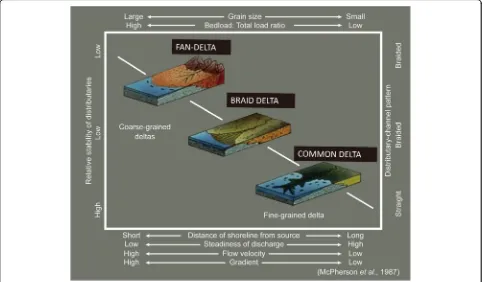
2.8 Fine-grained deltas versus coarse-grained deltas
In the geologic and engineering literature, the focus of
discussion
on
hyperpycnal
flows
is
centered
on
fine-grained deltas or common deltas. McPherson et al.
(
1987
)
distinguished
fine-grained
deltas
from
coarse-grained deltas (Fig.
5
). The importance here is
that braid (braided) deltas, kind of coarse-grained deltas,
are typical of high-gradient settings with high-velocity
river flows (Fig.
5
). Because these braided rivers plunge
into a standing body of water with multiple entry points,
separated by braided bars, these rivers develop linear
hyperpycnal plumes (Fig.
6
). Distinguishing linear types is
important because braid deltas are known to develop
vari-ous types of sediment flows, including debris flows, in the
subaqueous delta fronts (McPherson et al.
1987
). At
present, coarse-grained deltas are totally ignored in
study-ing hyperpycnal flows. As a consequence, all published
ex-amples of hyperpycnal lows are from fine-grained deltas,
such as the Yellow River delta in China.
3 The Yellow River, China
The Yellow River, which is the second largest river in
China, is regarded as the world
’
s largest contributor of
fluvial sediment load to the ocean (Yu et al.
2011
).
His-torically, it contributed a sediment load of nearly 100
million tons per year (Milliman
2001
). The Yellow
Riv-er
’
s average annual suspended-load concentration of
25,000 mg
⋅
L
−1and flood stage concentration of 220,000
mg
⋅
L
−1are the largest in the world by 1983 (Milliman
and Meade
1983
). In September 1995, a cruise was
undertaken to detect hyperpycnal flows off the Yellow
River mouth (Wang et al.
2010
). During the cruise
(18
–
19
September),
daily
suspended
sediment
Fig. 5A comparison of coarse-grained deltas and fine-grained deltas based on distributary-channel patterns and stability, sediment load and size,
concentration (SSC) was close to 50 kg
⋅
m
−3and daily
average stream discharge was 2000 m
3⋅
s
−1. The critical
concentration of suspended sediment ranges from 36
kg
⋅
m
−3to 43 kg
⋅
m
−3for coastal waters depending on
local salinity, temperature and climatic conditions
(Mulder and Syvitski
1995
).
The Yellow River drains through that part of the world
that is covered by extensive soft and easily erodible,
wind-transported, loess deposits in China (Fig.
7a
). The
loess is intensively eroded during the monsoon rains,
gen-erating unusual suspended particle concentration at the
Yellow River mouth, which generates hyperpycnal flows
(Wright et al.
1986
,
1990
). Because the Yellow River is an
ideal river for generating hyperpycnal flows, I focus
atten-tion on this river, which is rich in empirical data (Fig.
7
).
3.1 Delta versus estuary
One confusing aspect of the Yellow River literature is
that some authors refer to the river mouth as a
“
delta
”
(Gao et al.
2014
; Wang et al.
2017
; among many others),
whereas others refer to it as an
“
estuary
”
(e.g., Hu et al.
1998
; Wang and Wang
2010
). The distinction between a
delta and an estuary is not trivial (Dalrymple
1992
;
Dal-rymple et al.
1992
; Shanmugam et al.
2000
). The Yellow
River cannot be both a delta and an estuary at the same
time. According to the Oxford Dictionaries (
2018
), the
term
“
estuary
”
is derived from a mid sixteenth century
Latin word
“
aestuarium
”
meaning tidal part of a shore
(
‘
estus
’
=
‘
tide
’
).
Fairbridge (
1980
) defined an estuary as
“an inlet of
the sea reaching into a river valley as far as the upper
limit of tidal rise”
. Whether the Yellow River is a delta
or an estuary is important here because estuaries are
not ideal candidates for transporting hyperpycnite
sedi-ments offshore. This is because of ebb and flood tides
and their bidirectional currents. In this study, the
Yel-low River is considered to be a river-dominated delta
with tidal influence.
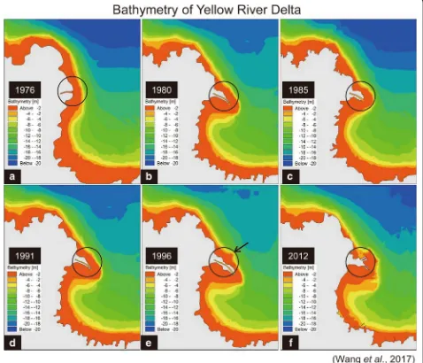
3.2 Bathymetry
Wang et al. (
2017
) obtained bathymetric data for the
Yellow River and the western Laizhou Bay for the years
1976, 1980, 1985, 1991, 1996 and 2012, and presented
maps with a spatial resolution of 300
–
500 m (Fig.
8
).
Maps show a clear change in bathymetry in front of the
river mouth because of the change in river course. The
change
in
river
course
from
an
abandoned
south-flowing old river (1976
–
1996) to the modern
north-flowing river was illustrated by Wang et al.
(
2015
, their Figs. 1 and 2e
–
f ). Changes in river-mouth
bathymetry are a reflection of chages in river courses
and related types of sediment plumes.
3.3 River-mouth processes
Wright et al. (
1986
) were the first authors to investigate
hyperpycnal flows at the Yellow River mouth. Because
the turbidite paradigm was in full force during the 1970s
and 1980s, Wright et al. (
1986
) emphasized the
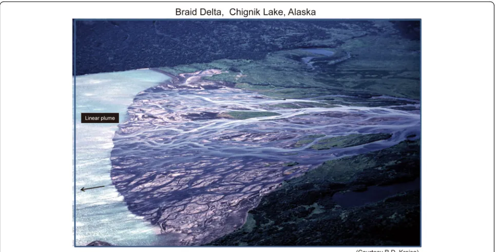
Fig. 6Braid delta from Chignik Lake, southeastern coast, Alaska, showing multiple entry points with shooting“linear”hyperpycnal plumes into a
standing body of water. Photo courtesy of R.D. Kreisa. From McPherson et al. (1987)
similarity between hyperpycnal flows and turbidity
cur-rents. As discussed earlier, turbidity currents are defined
on the basis of fluid rheology, flow state, and sediment
concentration, whereas hyperpycnal flows are defined
solely on fluid density.
The following is a compilation of types of flows that
have been used for the Yellow River.
1) Hyperpycnal underflow (Wright et al.
1986
).
2) Low-density hyperpycnal plume (Wright et al.
1986
).
3) High-density hyperpycnal plume (Wright et al.
1986
).
4) Tide-modulated hyperpycnal flow (Wang et al.
2010
).
5) Hyperconcentrated flow (van Maren et al.
2009
).
6) High-turbid mass flow (Fan et al.
2006
).
7) Turbidity current (Wright et al.
1986
).
Clearly, there is no consistency in term of fluid
dy-namics. From a practical point of view, none of these
publications discusses the depositional characteristics of
various types of hyperpycnal flows.
3.4 Bottom-turbid layers
Wright et al. (
2001
) suggested the influence of ambient
currents and waves on gravity-driven sediment flows,
which are different from hyperpycnal flows. In this
con-text, Gao et al. (
2015
) suggested that the Yellow River
has undergone a regime shift in response to
resuspen-sion induced by tidal currents and waves. This shift has
presumably resulted in the replacement of hyperpycnal
flows by bottom-turbid layers. The difference between
the two is that hyperpycnal flows behave as a single
Fig. 7Data from the Yellow River.aThe course of the Yellow River draining the loess plateau before entering the Bohai Bay. Note river mouth is
layer without vertical stratification in density or velocity
(Fig.
4a
), whereas bottom-turbid layers reveal vertical
stratification in density and velocity (Fig.
4b
). Such a
vertical stratification in bottom-turbid layers is similar
to the concept of
“
high-density turbidity current
”
(Postma et al.
1988
, their Fig. 2). The problem here is
that stratified high-density turbidity currents are sandy
debris flows because of their basal plastic layers
in-duced by high sediment concentration (Shanmugam
1996
). In support of a debris flow, Gao et al. (
2015
,
their Fig. 5b) depicted a
“
detached point
”
where the
flow front is lifted up from the seafloor (Fig.
4b
, the red
arrow).
This
phenomenon
is
identical
to
the
experimental debris flow with a detached and lifted-up
front due to hydroplaning (Mohrig et al.
1998
, their
Fig. 3; see also Shanmugam
2000
, his Fig. 15).
Although clearly implied, Gao et al. (
2014
,
2015
) did
not cite the pioneering work of Mohrig et al. (
1998
)
on hydroplaning.
3.5 Multi-layer hyperpycnal flows
Morales de Luna et al. (
2017
) simulated numerically a
multi-layer model for hyperpycnal flows on theoretical/
mathematical basis (Fig.
4c
). By contrast, Gao et al.
Fig. 8Maps showing changes in bathymetry of the Yellow River Delta through time. Note changes in shallowest (red) areas surrounding the river
mouth within the circle. The old Yellow River course that existed during 1976−1996 was abandoned and a modern river course was established since 1996 (Wang et al.2015, their figure 1). Note a slight protrusion to the north in red area (arrow) for the year 1996 caused by the change in river course (see Fig.2e). Images from Wang et al. (2017), with permission from Elsevier. Copyright Clearance Center’s RightsLink: Licensee: G. Shanmugam. License Number: 4258871156757. License Date: December 30, 2017. Additional labels by G. Shanmugam
(
2015
, their Fig. 5a) considered hyperpycnal flows as a
single-layer phenomenon on the empirical basis (Fig.
4a
).
The problem is that no one has ever documented
multi-layer hyperpycnal flows in natural environments.
Another problem is that Morales de Luna et al. (
2017
)
have applied the multi-layer model to both hyperpycnal
and hypopycnal plumes. Such applications of numerical
modeling to both types of density plumes raise the
question on the validity of numerical modeling when there
are no empirical bases for the existence of multi-layer
hyperpycnal flows in nature. This numerical approach is
akin to inventing medicine for a hypothetical disease that
does not exist.
3.6 Tide-modulated hyperpycnal flows
The term
“
tide-modulated hyperpycnal flow
”
(Fig.
4d
;
Wang et al.
2010
) is confusing. The reason is that
hyper-pycnal flows are unidirectional (i.e., travel seaward),
whereas tidal currents are bidirectional (i.e., travel both
seaward (ebb tide) and landward (flood tide)). In this
scenario, it is incongruous to mix tidal currents with
hyperpycnal flows in the same nomenclature. In
main-taining clarity, any current generated by tides should be
called a tidal current.
3.7 Internal waves
Wang et al. (
2010
; see also Wright et al., 1986)
sug-gested internal waves but did not provide empirical
evidence for internal waves at the mouth of the Yellow
River (Fig.
4d
). Internal waves are a complicated
oceanographic phenomenon (Shanmugam
2013
). For
example, internal waves occur only along pycnoclines
(Shanmugam
2013
), but there is no evidence of
pycno-clines at shallow depths where hyperpycnal plumes
de-velop in front of the Yellow River.
In summary, publications on the river-mouth
pro-cesses of the Yellow River have perpetuated unnecessary
conceptual problems by proposing complex processes
without empirical basis.
3.8 Velocity measurements
In their study on the Yellow River, Wright et al. (
1990
)
re-ported that strong (
∼
1 m
⋅
s
−1) parabathic tidal currents
re-suspended newly deposited muds and advected them
alongshore. It appears that tidal currents are more
power-ful than hyperpycnal flows. The velocity values used in
nu-merical modeling studies are from tidal currents (e.g.,
Wang et al.
2010
). Disappointingly, there are no empirical
data on velocity measurement of hyperpycnal flows from
the Yellow River mouth (Wright et al.
1986
).
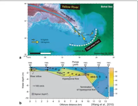
3.9 Tidal shear front
Perhaps the most significant contribution on the dynamics
of the Yellow River sedimentation is pertaining to the
recognition of tidal shear front (Fig.
9a
). Li et al. (
2001
),
based upon in-situ measurements and Landsat scanning
images, studied spatial
–
temporal changes in the shear
front and associated sedimentation in the subaqueous
delta slope of the Yellow River. The results showed that
the shear front is an important dynamic factor in
control-ling rapid accretion at the Yellow River mouth. Suspended
sediment converges and is deposited rapidly along the
shear front zone. This is because a low-velocity zone is
formed between two inverse flow bodies.
Qiao et al. (
2008
), by combining a three-dimensional
tidal front numerical model and a sediment transport
module, explained the formation of a tidal shear front
that occurs off the Yellow River mouth. Wang et al.
(
2010
) documented the position of the tidal front about
5 km seaward off the Yellow River mouth (Fig.
9a
) and
explained the tide-induced density flows on the shelf
(Fig.
9b
). The importance of these numerical
experi-ments is that the topography with a strong slope off the
Yellow River mouth was a determining factor on the
generation of a shear front.
The sedimentologic implication of the shear front is
that it limits seaward transport of sediments (Li et al.
2001
; Qiao et al.
2008
; Wang et al.
2007
,
2010
,
2017
). If
so, the extent of sediment transport into the deep sea by
hyperpycnal flows comes into question. In other words,
the entire concept of hyperpycnal flows transporting
sediment into the deep sea (Mulder et al.
2003
; Steel
et al.
2016
; Warrick et al.
2013
; Zavala and Arcuri
2016
)
is unsupported by the Yellow River, which is considered
to be a classic river for hyperpycnal flows.
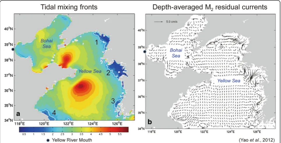
3.10 M2
tidal dynamics in Bohai and yellow seas
Wiseman et al. (
1986
) were one of the early workers
who recognized the importance of M
2tidal constituents
in the Bohai Sea. Yao et al. (
2012
) conducted a modeling
study of M
2tidal dynamics in understanding the
re-gional tidal mixing and tidal residual currents. There are
four regions of low values of log
10(
h
/
U
3): The inner shelf
of Seohan Bay, Kyunggi Bay, the shelf area off the
south-west Korean peninsula, and the China shelf area between
34°N and 35°N (Fig.
10a
). All these mixing zones are
confined in the Yellow Sea (Fig.
10a
). Inside the Bohai
Sea, strong residual currents are seen off the Yellow
River mouth (Fig.
10b
), near Liaodong Bay and north of
the Bohai Strait (Fang and Yang
1985
). From the above
empirical and numerical data, it is clear that the Yellow
River mouth is part of a regional tidal setting that
com-prises both Bohai Sea and Yellow Sea (Fig.
10
).
In summary, hyperpycnal flows are not simple
pro-cesses that begin their journey at plunge points,
trans-porting sediment across the shelf, and end up in the
deep sea. They are invariably affected by external
tidal currents on hyperpycnal flows is well documented
in the next case study, which is the Yangtze River.
4 The Yangtze River, China
4.1 Hyperpycnal and hypopycnal plumes
The Yangtze River is the longest river (about 6,300 km)
in Asia. Satellite images show that the Yangtze River
generates both hyperpycnal and deflected hypopycnal
plumes (Fig.
11a
). The Yangtze River mouth is a complex
setting in which both ocean currents and tidal currents
are affecting sediment dispersal.
4.2 Ocean currents
Unlike the Yellow River that enters a protected Bohai Bay
from major ocean currents, the Yangtze River enters the
East China Sea affected by the warm, north-flowing
Kuro-shio Current (Fig.
11b
). As a consequence, muddy
sediments brought by the Yangtze River are redistributed
and deposited as a mud belt on the inner shelf (Wu et al.
2016
). This mud belt is evident on the satellite images
(Fig.
11a
). This mud belt is distinctly different from the
fan-shaped or lobate deposits of hyperpycnal flows
associ-ated with the Yellow River (Fig.
2e
). Liu et al. (
2006
)
pro-posed a sediment dispersal model by ocean currents for
sediments supplied into the East China Sea by the Yangtze
River (Fig.
11c
). Ocean currents are a global phenomenon
(Talley
2013
) with implications for sediment distribution
in the world
’
s oceans (Shanmugam
2017b
).
4.3 Tidal river dynamics
Similar to the Yellow River, both terms
“
delta
”
and
“
estu-arine
”
are used for the Yangtze River mouth (e.g., Liu
et al.
1992
). However, evidence for a tide-dominated
es-tuary is compelling.
Fig. 9Tidal shear front.aSatellite image showing the sediment dispersal pattern at the Yellow River mouth and estimated mean depth-integrated
sediment flux at six stations in 1995 cruise. Note a tidal shear front (white dashed line);bDistributions of bulk density along a transect through the six stations on 18 September 1995, demonstrating the spatial pattern of a flow extending seaward beneath the ambient sea water. Both from Wang et al. (2010), with permission from John Wiley and Sons. Copyright Clearance Center’s RightsLink: Licensee: G. Shanmugam. License Number: 4258840606863. License Date: December 30, 2017. Additional labels by G. Shanmuagam
Hoitink and Jay (
2016
) reviewed tidal river dynamics of the
world
’
s rivers and classified the Yangtze as a
“
tidal river
”
.
Guo et al. (
2015
) documented that the tidal influence
(salt-wedge intrusion) can extend to Datong, which is
650 km upstream from the river mouth (Fig.
12a
).
Guo et al. (
2014
) documented river-mouth bars
(Fig.
12b
) that are analogous to tidal sand bars (Dalrymple
et al.
1990
). Liu et al. (
1992
) reported the development of
estuarine sand bars. In support of this observation, a 1997
bathymetric map reveals river-mouth bars, mimicking
tidal sand bars typical of tide-dominated estuaries (see
Dalrymple et al.
1990
; Shanmugam et al.
2000
).
Guo et al. (
2015
) documented the changes in mean
water level at Datong with respect to discharge
associ-ated with tides (Fig.
12c
).
Tides in the Yangtze River Estuary are semidiurnal
with the average tidal range of 2.76 m and the maximum
of 4.62 m (Lu et al.
2015
) or 5.0 m (Chen et al.
1998
).
Tidal flow velocity at the river mouth was measured to
be 1 m
⋅
s
−1(Milliman et al.
1985
).
Hori et al. (
2002
) proposed a tide-dominated delta
with sand
–
mud couplets and bi-directional cross
lami-nations for the Yangtze Holocene succession.
The differences between a common river and a tidal
river affect sedimentation at plunge points (Fig.
12d
).
For example, unlike river-dominated deltas with
unidir-ectional
sediment
transport
(i.e.,
seaward),
tide-dominated estuarine systems are prone to
bidirec-tional transport of sediment (i.e., both seaward and
land-ward) (Dalrymple
1992
; Dalrymple et al.
1992
). Under
such conditions, the idea of sediment transport by
hyperpycnal flows from the river mouth to the deep sea,
traveling across the shelf, is misleading.
Although both the Yellow and the Yangtze Rivers
de-velop hyperpycnal lows at their river mouths, transport
of hyperpycnal sediments from the river mouth to the
deep sea has been blocked or diverted by different
exter-nal controls, such as tidal shear front and ocean currents
(Fig.
13
). This important oceanographic control has been
overlooked in studies of hyperpycnites (e.g., Zavala and
Arcuri
2016
). In this review, 15 external controls have
been identified from global case studies (see Section
5
).
5 External controls
External controls are allogenic in nature, which are
ex-ternal to the depositional system, such as uplift,
subsid-ence, climate, eustacy, etc. However, external controls of
density plumes are much more variable and include
some
common
depositional
processes
(e.g.,
tidal
Fig. 10Tidal data.aTidal mixing parameter log10(h/U
3
) for M2tidal currents, wherehis the local water depth in meter andUis the depth-averaged
tidal velocity in meter per second. Solid, white contour lines indicate log10(h/U 3
) = 2.0, which defines tidal mixing fronts at four locations: (1) the inner shelf of Seohan Bay, (2) Kyunggi Bay, (3) the shelf area off the southwest Korean peninsula, and (4) the China shelf area between 34°N and 35°N;b Map showing depth-averaged M2residual currents. Note strong residual currents are seen off the Yellow River mouth. The tidal residual vectors are
plotted every 5 grid points. M2(period: 12.42 h): Main lunar semidiurnal constituent (see Shanmugam2012, Appendix A for explanations of tidal
currents). At least, 15 external controls of plumes have
been recognized in this review (Table
1
):
1) Tidal shear front (Fig.
9
): The Yellow River
(Wang et al.
2010
).
2) Ocean currents (Fig.
11
): The Yangtze River (Liu
et al.
2006
).
3) Tidal currents (Table
1
): San Francisco Bay
(Barnard et al.
2006
; NASA
2017
).
4) Monsoonal currents (Jagadeesan et al.
2013
).
5) Wave action (Hawati et al.
2017
).
6) Cyclones (Table
1
): Gulf of Mexico; U.S. Atlantic
shelf (Shanmugam
2008a
,
2008b
).
7) Tsunamis (Table
1
): Sri Lanka, Arabian Sea
(Shanmugam
2006b
).
8) Braid delta and related high gradients and coarse
sediments
(Fig.
6
):
Alaska,
Pacific
Ocean
(McPherson et al.
1987
).
Fig. 11Data from the Yangtze River.aSatellite image showing the Yangtze River plunging into the East China Sea. Note development of both
hyperpycnal plume (yellow color due to high sediment concentration) near the river mouth and hypopycnal plume (blue color due to low sediment concentration) on the seaward side. Note deflected hypopycnal flows that move southward (white arrow), possibly due to modulation by south-flowing shelf currents. In a recent study, Luo et al. (2017) recognized that extended and deflected density plumes (white arrow) tend to develop during winter months, which are absent during the summer months. Note sheet-like mud belt developed along the inner shelf due to contour-following shelf currents. White dashed circle = River mouth. See Fig.12afor the river course; see also Fig.7a. River image credit: NASA Visible Earth, Jacques Descloitres, MODIS Land Science Team.https://visibleearth.nasa.gov/view.php?id=55219. Image acquired on September 16, 2000. Instrument: Terra-MODIS;bMap showing warm Kuroshio Current (KC) in the East China Sea and Yellow Sea. TWC = Taiwan Warm Current; YSWC = Yellow Sea Warm Current; ZFCC = Zhejiang−Fujian Coastal Current; JCC = Jiangsu Coastal Current. Blue circles: Yangtze and Yellow River mouths. From Liu et al. (2006) with additional labels by G. Shanmugam;c Conceptual model of sedimentary and oceanographic processes affecting the sediment dispersal at both subaqueous delta and alongshore deposits associated with the Yangtze River. From Liu et al. (2006) with additional labels by G. Shanmuagm. Both B and C figures with permission from Elsevier. Copyright Clearance Center’s RightsLink: Licensee: G. Shanmugam. License Number: 4258820168883. License Date: December 30, 2017
9) Seiche in lakes (Table
1
): Lake Erie (NASA
2017
).
Seiche is a large standing wave that occurs when
strong winds and a quick change in atmospheric
pressure push water from one end of a body of
water to the other. de Jong and Battjes (
2004
)
discussed the atmospheric origin of seiche.
10) Upwelling (Table
1
): Off Namibia (Shillington
et al.
1992
).
11) Fish activity (Table
1
): The Great Bahama Bank
(Broecker et al.
2000
).
12) Volcanic eruptions (Table
1
): Bering Sea (NASA
2017
).
13) Coral
reef
(Table
1
):
South
Pacific
Ocean
(NASA
2017
).
14) Pockmarks:
Carolina
Continental
Rise,
North
Atlantic Ocean (Paull et al.
1995
).
15) Internal waves and tides (Masunaga et al.
2015
).
Fig. 12Tidal data. aThe Yangtze River estuary and the location of the tidal gauge stations (red filled circles). The numbers in brackets are
I have discussed the importance of external controls,
such as tidal shear front and ocean currents earlier.
Fu-ture studies should consider external controls in
developing meaningful depositional models.
6 Recognition of ancient hyperpycnites
Recognition of ancient hyperpycnites is rare. However,
there are studies that claim that hyperpycnites can be
recognized using various criteria. In the following
dis-cussion, problems associated with recognizing ancient
hyperpycnites are identified.
6.1 The hyperpycnite facies model
Mulder et al. (
2003
) proposed a facies model for
hyper-pycnites (Fig.
14a
). This model is based on a hypothesis
that hyperpicnite facies is a function of the magnitude of
the flood at the river mouth. According to this hypothesis,
hyperpycnites accurately record the rising and falling
dis-charge of a flooding river in terms of sediment-size,
in-verse grading to normal grading in ascending order
(Fig.
14a
), primary sedimentary structures, bed thickness,
and erosional contacts. Mulder et al. (
2003
) were the first
authors to propose a facies model with an internal
ero-sional surface (Fig.
14a
).
In testing Mulder et al. (
2003
) hypothesis, Lamb et al.
(
2010
) conducted laboratory flume experiments and
concluded that the hypothesis is unsupported by
experi-mental results. Furthermore, Clare et al. (
2016
) reported
that the largest river discharges did not create
hyperpyc-nal flows based on field monitoring of the Squamish
Delta, British Columbia, Canada during 2011, thus
dis-puting the hypothesis.
Although ichnological signatures (i.e., bioturbation and
trace fossils) are claimed to be characteristic features of
hyperpycnites (Buatois et al.
2011
) and contourites (Stow
and Faugères,
2008
), skepticism about these claims exists
(Shanmugam,
2002
,
2018d
).
6.2 Inverse to normal grading
Following the concept of Mulder et al. (
2003
), Wilson and
Schieber (
2017
) and Yang et al. (
2017a
) recognized ancient
hyperpycnites based on inverse to normal grading.
How-ever, the origin of inverse grading by waxing flows is an
unresolved issue (Shanmugam
2002
). For example,
mech-anisms which are commonly used to explain inverse
grad-ing are (1) dispersive pressure, caused by grain-to-grain
collision which tends to force larger particles toward the
zone of least rate of shear (Bagnold
1954
), (2) kinetic
siev-ing, by which smaller particles tend to fall into the gaps
between larger particles (Middleton
1967
), and (3) the lift
of individual grains towards the top of flow with lower
pressures (Fisher and Mattinson
1968
). Nevertheless,
Mulder et al. (
2001
) did not consider any of these
alterna-tive mechanisms.
Yang et al. (
2017a
) recognized normal grading in the
Triassic Yanchang Formation in the Ordos Basin,
Central China, and interpreted normal grading as
Fig. 13Comparison of conceptual diagrams showing differences in depositional models betweenathe Yellow River andbthe Yangtze River.
Note external controls on the distribution of muddy hyperpycnites. In the Yellow River, a tidal shear front prevents seaward transport of sediment. In the Yangtze River, ocean currents deflect plumes and deposit them as inner-shelf mud belt
hyperpycnite (Fig.
14b
). However, normal grading in the
Yanchang Formation was previously interpreted as
turbi-dites (Zou et al.
2012
).
Wilson and Schieber (
2014
,
2017
) described a muddy
unit with normal to inverse grading in ascending order
from the Devonian Lower Genesee Group, Central New
York, which they interpreted as hyperpycnites. These
muddy units were previously interpreted as turbidites by
other researchers. Muddy turbidity currents and
hyper-pycnal flows are one and the same, according to some
authors (see Kostic and Parker
2003
; Lamb et al.
2010
).
As explained earlier, it is wrong to equate hyperpycnal
flows with turbidity currents on fluid dynamical
princi-ples (see Section
2
).
6.3 Internal erosional surface
Following Mulder et al. (
2003
), Yang et al. (
2017a
) claimed
that internal erosional surfaces, which occur between
basal inversely graded layer and upper normally graded
layer, are the diagnostic criteria of hyperpycnites (Fig.
14b
).
Conventionally, a genetic facies model is designed for a
single depositional event, without internal hiatuses. A
classic example is the turbidite facies model or the
“
Bouma Sequence
”
(Bouma
1962
). In fact, Walther
’
s Law
(Middleton
1973
) is not meaningful for sequences with
in-ternal hiatuses. This is because a hiatus can represent a
considerable span of time (spanning millions of years) that
is missing along an erosional surface (Howe et al.
2001
).
Therefore, it is sedimentologically meaningless to relate
Fig. 14Facies models and features.aHyperpycnite facies model showing inverse to normal grading with erosional contact in the middle. From