Bayesian Fairness

The Thirty-Third AAAI Conference on Artificial Intelligence (AAAI-19)

Bayesian Fairness

Christos Dimitrakakis,

Yang Liu,

David C. Parkes,

Goran Radanovic

[email protected], [email protected], [email protected], [email protected]

Abstract

We consider the problem of how decision making can be fair when the underlying probabilistic model of the world is not known with certainty. We argue that recent notions of fairness in machine learning need to explicitly incorporate parameter uncertainty, hence we introduce the notion ofBayesian fair-nessas a suitable candidate for fair decision rules. Using bal-ance, a definition of fairness introduced in (Kleinberg, Mul-lainathan, and Raghavan 2016), we show how a Bayesian per-spective can lead to well-performing and fair decision rules even under high uncertainty.

Introduction

Fairness is an important property of algorithmic systems in settings where decisions are made that affect individuals in a population, for example in the context of loan decisions, college admissions, hiring decision, or bail decisions.

Recognizing this, there has been considerable emphasis in recent work on developing definitions of fairness in the context of machine learning algorithms. In this paper, we take a closer look at informational aspects of fairness. In particular, by adopting a Bayesian viewpoint, we explicitly take into account model uncertainty, something that turns out to be crucial for fairness.

Uncertainty about the underlying probabilistic model of the world has two main effects. Firstly, many notions of fair-ness have been defined with respect to latent variables, in-cluding model parameters. This means that we need to take into account uncertainty about these latent variables and pa-rameters. Secondly, in many problems our decisions deter-mine the data that we will collect in the future. Ignoring un-certainty may magnify subtle biases in our model.

By viewing fairness through a Bayesian perspective, we avoid these problems. In particular, we demonstrate that Bayesian policies can allow for suitable trade offs to be made between utility and fairness, taking into account un-certainty about model parameters.

We consider a setting where a decision maker (DM) makes a sequence of decisions through some chosenpolicy

πto maximize herexpected utilityu. However, the DM must trade off utility with somefairness criterionf. We assume

Copyright c⃝2019, Association for the Advancement of Artificial Intelligence (www.aaai.org). All rights reserved.

the existence of some underlying probability lawP, so that the decision problem, whenP is known, can be written as:

max

π (1−λ)E π

Pu−λE π

Pf, (1)

whereλis the DM’s trade-off between fairness and utility.1 We adopt a Bayesian viewpoint and assume the DM has be-liefβover some family of distributionsP_,{Pθ|θ∈Θ}, which may contain the actual law, i.e.Pθ∗=Pfor someθ∗. The DM’s policyπdefines the actionsat ∈ Athe DM takes at different (discrete) timestdepending on the avail-able information. More precisely, at timetthe DM observes somedataxt ∈ X, and depending on her beliefβtmakes adecisionat ∈ A, so thatπ(at | βt, xt)defines a proba-bility over actions for every possible belief and observation. The DM has a utility function, modeled here with structure

u : A × Y → _R, whereY is a set ofoutcomes(in a loan setting, was the loan repaid on time?). The fairness concept we focus on is a Bayesian version of balance (Kleinberg, Mullainathan, and Raghavan 2016), which is also a gener-alization of the equality of opportunity (Hardt, Price, and Srebro 2016).

The amount of uncertainty about the model parameters di-rectly influences the interpretation of the balance condition. Informally, the more uncertain we are, the more stochastic the decision rule will need to be.

Our contributions. In this paper, we develop a Bayesian framework for fairness that recognizes that there can be a high degree of uncertainty about model parameters and la-tent variables, and especially when not a lot of data has been collected, or in sequential settings. In particular, we propose that the DM should take into account how unfair she would be under all possible models, weighted by their probability. Fairness is a property of the decision rule with respect to the true model, and it is this that is used tomeasurefairness. On the other hand, the appropriate way to achieve fairness de-pends on the DM’s information, and it is this that is used to derivealgorithms. In order to work without model approx-imations, we illustrate the approach in a simple setting. We show that the policies that are obtained are qualitatively and

1

quantitatively different when we consider uncertainty and adopt a Bayesian viewpoint in comparison to when we do not.

Given that the Bayesian approach to fairness takes into account uncertainty and makes explicit consideration of the DM’s information, we can also use the approach to select policies that influence the data we collect, and thus our knowledge about the model. This is an important informa-tional feedback effect, and one that a Bayesian methodology can provide in a principled way. We provide experimental results on the COMPAS dataset (Larson et al. 2016) as well as artificial data, showing the robustness of the Bayesian approach, and comparing against methods that define fair-ness measures according to a single, marginalized model (e.g. (Hardt, Price, and Srebro 2016)). While we mainly treat the non-sequential setting, where the data is fixed, we can also accommodate sequential, bandits-style settings, as ex-plained in later sections. The results there provide a vivid il-lustration of what can go wrong with a certainty-equivalent approach to achieving fairness.

All missing proofs and details can be found in our supple-mentary materials.

Related work. Algorithmic fairness has been studied quite extensively in recent work. But we are not aware of work that adopts a Bayesian perspective. For instance, (Dwork et al. 2012; Chouldechova 2016; Corbett-Davies et al. 2017; Kleinberg, Mullainathan, and Raghavan 2016; Kilbertus et al. 2017) studied fairness under a setting where the model is known. (Corbett-Davies et al. 2017) have con-sidered how to satisfy fairness considerations while also maximizing expected utility. In this paper, we focus on no-tions of fairness related to nono-tions of conditional indepen-dence, the specifics of which are discussed in the next sec-tion.

(Dwork et al. 2012) consider an individual-fairness ap-proach, and look for decision rules that are smooth in a sense that similar individuals are treated similarly.

The recent work of (Russell et al. 2017) considers the problem of uncertainty from the point of view of causal modeling, with the three main differences to the present work being: (a) they consider a PAC-like setting, rather than the Bayesian framework; (b) we show that the effect of uncertainty remains important even without varying the counterfactual assumptions; and (c) the Bayesian frame-work easily admits a sequential setting. (Jabbari et al. 2016) and (Joseph et al. 2016) study fairness in sequential decision making settings, but not from a Bayesian viewpoint.

There is also research on questions of fairness in other machine learning contexts, such as clustering (Chierichetti et al. 2017), natural language processing (Blodgett and O’Connor 2017) and recommendation systems (Celis and Vishnoi 2017).

Preliminaries

(Chouldechova 2016) considers the problem of fair predic-tion with disparate impact. She defines an acpredic-tion (a “statis-tic” in her paper)aastest-fairwith respect to theoutcome

yandsensitive variablezifyis independent ofzunder the action and parameterθ, i.e. ify⊥⊥z|a, θ. While the author does not explicitly discuss the distributionPθ, it is implicitly assumed to be that of the true model. We slightly generalize the definition of disparate impact as follows:

Definition 1 (Calibrated decision rule). A decision rule

π(a | x)iscalibratedwith respect to some distributionPθ ify, zare independent for all actionsataken, i.e. if

P_θπ(y, z |a) =P_θπ(y|a)P_θπ(z|a), (2) wherePπ

θ is the distribution induced byPθand the decision ruleπ.

(Kleinberg, Mullainathan, and Raghavan 2016) also con-sider two balance conditions (one for each label class), which we re-interpret as follows. Here, we simplify the no-tation of the decision rule so thatπ(a|x)corresponds to the probability of taking actionagiven observationx.

Definition 2(Balanced decision rule). A decision ruleπ(a| x)isbalancedwith respect to some distributionPθ ifa, z are independent for ally, i.e. if

P_θπ(a, z |y) =P_θπ(a|y)P_θπ(z|y), (3) whereP_θπis the distribution induced byPθand the decision ruleπ.

As with (Chouldechova 2016), (Kleinberg, Mullainathan, and Raghavan 2016) also work with the true model. We will slightly generalize the definition, stating balance with re-spect to any model parameter.

It is known that calibration and balance cannot be achieved simultaneously for non-trivial environments (Kleinberg, Mullainathan, and Raghavan 2016; Choulde-chova 2016). This is also true for our more general defini-tions, as we show in Theorem S1 in the Supplementary ma-terial.

From a practitioner’s perspective, we must choose either calibration or balance. We work with a generalized version of the balance condition, because balance gracefully extends to settings with uncertainty. In particular, balance involves equality in the expectation of a score function (when writ-ing the probabilities as the expectations of a 0-1 indicator function; also depending on an observationx) under differ-ent values of a sensitive variablez, conditioned on the true (but latent) outcomey. Consequently, balance can always be satisfied—by using a randomized decision rule that is inde-pendent of x. This is not the case for the calibration con-dition under model uncertainty, because calibration criteria depends highly on the details of a model.

Bayesian Formulation

We first introduce a concrete, statistical decision problem. The true (latent) outcome y is generated independently of the DM’s decision, with a probability distribution that de-pends on the available information x. There also exists a sensitive attribute variable z, which may be dependent on

x.2

2

β θ

z x

y u

a π

Figure 1: A Bayesian decision problem with observationsx, outcomey, actiona, sensitive variablez, utilityu, unknown parameter θ, belief β and policyπ. The joint distribution ofx, y, zis fully determined by the unknown parameter θ, while the conditional distribution of actionsagiven obser-vationsxis given by the selected policyπ. The DM’s utility function isu, while the fairness of the policy depends on the problem parameters.

Definition 3(Statistical decision problem). See Figure 1 for the decision diagram. The DM observesx∈ X, then takes a decisiona ∈ Aand obtains utilityu(y, a)depending on a true (latent) outcome y ∈ Y generated from some dis-tribution Pθ(y | x). The DM has a belief β ∈ B in the form of a probability distribution on parametersθ ∈ Θ on a familyP _,{Pθ(y|x)|θ∈Θ}of distributions. In the Bayesian case, the belief β is a posterior formed through a prior and available data. The DM has a utility function

u:Y × A →_R, with utility depending on the DM’s action and the outcome.

For simplicity, we will assume thatX,A, andY, are finite sets, whereasΘis a subset of_Rn_{. We focus on Bayesian} de-cision rules, i.e. rules whose dede-cisions depend upon a pos-terior belief β. The Bayes-optimal decision rule, ignoring fairness, is defined below.

Definition 4 (Bayes-optimal decision rule). The Bayes-optimal decision ruleπ∗ _{: B × X → Ais a deterministic}

policy that maximizes the utility in expectation, i.e. takes action π∗(β, x) ∈ arg max_a∈Auβ(a | x), with uβ(a |

x)_,∑

yu(y, a)Pβ(y|x), wherePβ(y|x),

∫

ΘPθ(y |

x) dβ(θ)is the marginal distribution over outcomes condi-tional on the observations according to the DM’s beliefβ.

The Bayes-optimal decision rule does not directly depend on the sensitive variablez. We are interested in settings with multiple time periods. At timet, the DM observesxtand makes a decision atusing policy πt and obtains some in-stantaneous payoffUt=u(yt, at)and fairness violationFt. The DM’s utility is the sum of instantaneous payoffs over time,U _,∑T

t=1u(yt, at)and she is interested in finding a policy maximisingU in expectation.

Although the Bayes-optimal decision rule brings the high-est expected reward to the DM, it may be unfair. In the se-quel, we will define analogs of thebalancenotion of fairness in terms of decision rulesπ, and investigate appropriate de-cision rules, that possibly result in randomized policies. In particular, we shall consider a utility function that combines the DM’s utility with the societal benefit that comes from fairness, and search for Bayes-optimal decision rules with respect to this new, combined utility.

In particular, we define a Bayesian analogue of the

maxi-mization problem (1) as:

max

π (1−λ)E π

βu−λE π βf

= max

π

∫

Θ

[(1−λ)_Eπ_θu−λ_Eπ_θf] dβ(θ). (4)

To make this concrete, in the sequel we shall define the appropriate Bayesian version of the balance condition.

Bayesian Balance

In the Bayesian setting, we would like our decisions to take into account their impact on all possible models. That is, fairness is measured with respect to the true model.

It turns out that sometimes only a trivial decision rule can satisfy a strong form of balance in a setting with model un-certainty. In particular, what if we insist that balance must hold exactly, for all possible model parameters?

Theorem 1. A trivial decision rule of the formπ(a| x) = pacan always satisfy balance for a Bayesian decision prob-lem. However, it may be the only balanced decision rule, even when a non-trivial balanced policy can be found for every possibleθ∈Θ.

The proof, as well as an example illustrating this result, are in the supplementary materials.

For this reason, we consider the thep-norm of the devia-tion from fairness with respect to our beliefβ:

Definition 5(Bayesian Balance). We say that a decision rule

πis(α, p)-Bayes-balanced with respect to beliefβif:

f(π)_, ∫

Θ

∑

a,y,z

⏐ ⏐ ⏐ ⏐

∑

x

π(a|x)[Pθ(x, z|y)

−Pθ(x|y)Pθ(z|y)]

⏐ ⏐ ⏐ ⏐

p

dβ(θ)≤αp. (5)

This definition captures the expected deviation from bal-ance of policyπ, for a Bayesian DM under their beliefβ. It measures the deviation of policyπfrom perfect balance with respect to each possible parameterθ, and weighs this devi-ation according to the probability of that model. This pro-vides a graceful trade-off between achieving near-balance in the most likely models, while avoiding extreme unfairness in less likely ones.

Why not use a single point estimate for the model, instead of the full Bayesian approach? This would entail simply measuring balance (and utility) with respect to the marginal model,Pβ,

∫

ΘPθdβ(θ).

Definition 6 (Marginal balance). A decision rule π(·) is

(α, p)-marginal-Balanced with respect to beliefβif∀a, y, z:

∑

a,y,z

⏐ ⏐ ⏐ ⏐

∑

x

π(a|x) [Pβ(x, z|y)−Pβ(x|y)Pβ(z|y)]

⏐ ⏐ ⏐ ⏐

p ≤α.

(6)

Still, both balance conditions can provide a bound on bal-ance with respect to the true model. For this, denote the true underlying model asθ∗_{, and define the(ϵ, δ)-accurate belief.}

Definition 7. We callβ(θ)an(ϵ, δ)-accurate belief with re-spect to the true modelθ∗∈Θ, if withβ-probability at least

1−δ,∀x, y, z:

|Pθ(x|y, z)−Pθ∗(x|y, z)| ≤ϵ, |P_θ(x|y)−P_θ∗(x|y)| ≤ϵ,

i.e. the setΘϵfor which the above conditions hold has mea-sureβ(Θϵ)≥1−δ.

Under some conditions, the balance achieved through ei-ther definition provides an approximation to balance under the true model, as shown by the following theorem.

Theorem 2. If a decision rule satisfies either (α,1) -marginal-balance or (α,1)-Bayes-balance for β or both, andβis(ϵ, δ)-accurate, then the resulting decision rule is a

(α+ 2|A| · |Z| · |Y| ·(ϵ+δ),1)-balanced

decision rule w.r.t. the true modelθ∗.

This theorem says that if our belief β is concentrated around the true modelPθ∗, and our decision rule is fair with respect to either definition, then it is also fair with respect to the true model.

The Sequential setting

We can also extend the approach to a sequential setting, where the information learned by the DM about the envi-ronment depends on the action.

For example, if we approve a loan, we will only later dis-cover if the loan is paid off on time. This information will in turn affect our future decisions. Analogous to other se-quential decision making problems such as Markov decision processes (Puterman 1994), we need to solve the following optimization problem over a time horizonT:

max

π Eβ1

[ T

∑

t=1

(1−λ)Ut−λFt

]

, (7)

whereπnow must explicitly map future beliefsβtto proba-bilities over actions. If the data that the DM obtains depends on her decisions at, then she must consider adaptive poli-cies, as the next belief depends on the data obtained by the policy.

We can reformulate the maximization problem so as to explicitly include the future changes in belief:

V∗(βt),sup πt

Eπtβt[(1−λ)Ut−λFt]

+∑

βt+1

V∗(βt+1)Pβπtt(βt+1), (8)

under the mild assumption that the set of reachable next be-liefs is finite (easily satisfied when the set of outcomes is finite). This now features the tradeoff between explore (ob-taining new knowledge) and exploit (maximizing utility).

However, just as in the bandits case (c.f. Duff 2002), the above computation is intractable, as the policy space is expo-nential inT. For this reason, in this paper we only consider

myopic policiesthat select a policy (and decision) that is op-timal for the current step t, trading utility and fairness as well as the value of the information at any particular single step. A specific instance of this type of sequential version of the problem is a later section.

Algorithms

We compare the Bayesian framework with the simpler, marginal-model approach. In particular, for the Bayesian framework, we directly optimize (4). Using the marginal simplification, we maximize (1) with respect to the marginal modelPβ.

Balance gradient descent

We have a family of models{Pθ}with a corresponding sub-jective distributionβ(θ). In order to derive algorithms, we shall focus on the quantity:

C(π, θ)_,∑

y,z

 

∑

x

π(a|x)∆θ(x, y, z)



_p, (9)

This isthe deviation from balance for decision ruleπ un-der parameterθ, where

∆θ(x, y, z),Pθ(x, z|y)−Pθ(x|y)Pθ(z|y). (10) Given this, the Bayesian balance of the policy isf(π) = ∫

ΘC(π, θ) dβ(θ).

In order to find a rule that trades-off utility for balance, we maximize a convex combination of the expected utility and deviation specified in (4). In particular, we look for a parametrized rule πw solving the following unconstrained maximization problem:

max

πw

∫

Θ

Vθ(πw) dβ(θ),

Vθ(πw),(1−λ)Eθπwu−λC(πw, θ) (11) To perform this maximization, we use parametrized poli-cies and stochastic gradient descent. In particular, for a finite setX andY, the policies can be defined in terms of param-eterswxa =π(a|x). Then we can perform stochastic gra-dient descent as detailed in the Supplementary materials, by samplingθ∼β, and calculating the gradient for each sam-pledθ. For the marginal decision rule, we employ the same approach, but instead of sampling the parameters from the posterior, we use the parameters of the marginal model.

Experiments

algorithm is generally applicable, and could be combined for example with MCMC inference.

Performance is evaluated with respect to the actual bal-ance and utility achieved: for the synthetic data this is mea-sured according to the actual data-generating distribution, while for the COMPAS data this is the empirical distribu-tion on a holdout set.

The algorithm for optimizing policies uses stochastic gra-dient descent. In particular, the Bayesian policy minimizes (5) by samplingθfrom the posterior distributionβand then taking a step in the gradient direction. The marginal policy simply performs steepest gradient descent for the marginal model.

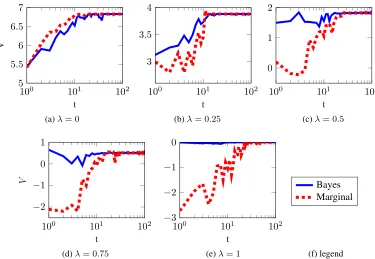
The results shown in Figures 2–5 display the performance of the corresponding Bayesian or marginal decision rule for different value ofλas more data is acquired. In the first two experiments, we assume that no matter what the decision of the DM is,zt, ytare always observed after the DM’s deci-sion and so the model is fully updated. In that setting, it is not necessary for the DM to take into account the informa-tion generated by acinforma-tions. However, in the third experiment, described below, the values ofztandytare only observed when the DM makes the decisionat= 1, and the DM faces a generalized exploration problem.

The model we employ throughout is a discrete Bayesian network model, with finiteX,Y,Z,A. The models are thus described through multinomial distributions that capture the dependency between different random variables. The avail-able data is used to calculate aposteriordistributionβ(θ). From this, we calculate both a marginal balanced rule as well as a Bayesian balanced rule. The former uses the marginal model directly, while the latter usesk = 16samples from the posterior distribution.3_{We tested these approaches both} on synthetic data and on the COMPAS dataset. The conju-gate prior distribution to this model is a Dirichlet-product. The graphical model is fully connected, and the model uses the factorizationPθ(x, y, z) =Pθ(y |x, z)Pθ(x|z)Pθ(z). We used this simple modeling choice throughout the paper, apart from the small experiment on synthetic data in the fol-lowing section (Experiments on synthetic data). In all cases where a Dirichlet prior was used, the Dirichlet prior param-eters were set equal to1/2.

Experiments on synthetic data

Here we consider a discrete decision problem, with|X |= 8, |Y| =|Z| = |A| = 2, andu(y, a) = I{y=a}. We gen-erate100observations from this model. We perform the ex-periment 10 times, each time generating data from a fully connected, discrete Bayesian network with uniformly ran-domly selected parameters. Unlike the rest of the paper, in this example, the prior distribution has finite support on only 8 models. This means that the posterior will have effectively converged to the true model after 100 observations.

As can be seen in Figure 2, the relative performance of the Bayesian approach w.r.t. the marginal approach increases

3

We found empirically that 16 was a sufficient number for sta-ble behaviour and efficient computation. Fork= 1the algorithm reduces to an approximation of Thompson sampling.

as we put more emphasis on fairness (Figure 2 (a) cares nothing about fairness.). In some cases (e.g. Figure 2 (c)), value for the marginal approach decreases at the beginning and eventually reaches the same value as the Bayesian ap-proach after enough data has been observed. This conforms with our hypothesis that one should take into account model uncertainty. The fact that both approaches converge toward the maximum value is in accordance with our formal results (Theorem 2).

Finally, Figure 3 and its extended version (Figure S1 in supplementary materials) more clearly shows how well the two different solutions perform with respect to the utility fairness trade-off. As we varyλand the amount of data, both methods achieve the same utility. However the Bayesian ap-proach consistently achieves lower fairness violations for similarU.

Experiments on COMPAS data

For the COMPAS dataset, we consider a discretization where fields such as the number of offenses are converted to binary features.4We used the first 6000 observations for training and the remaining 1214 observations for validation. Two attributes are sensitive (sex, race), while six attributes (relating to prior convictions and age) are used for the pol-icy. With discretization, there are a total of 12 distinct val-ues for the sensitive attributes and 141 for the features that are used for the underlying model. The task is to predict re-cidivism over the next two years, with DM utility function

u(a, y) =I{a=y}.

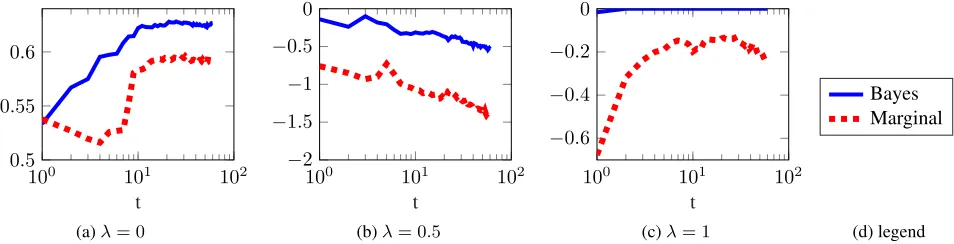
Figure 4 and its extended version (Figure S2 in the supple-mentary materials) show the results of applying our analysis to the COMPAS dataset used by ProPublica. Since in this case the true model is unknown, the results are calculated with respect to the marginal model estimated on the holdout set. In this scenario we can see that when we only focus on classification performance, the marginal and Bayesian deci-sion rules perform equally well. However, when we place more emphasis on fairness, we observe that the Bayesian approach dominates.5

Sequential allocation

Suppose now that the DM, at each timet, observesxtand has a choice of actions at ∈ {0,1}. Both actions are to predict whether yt ∈ {0,1} and have the following side-effect: the DM only observes yt, ztupon decisionat = 1, and otherwise only observes xt. The utility is not directly observed by the DM, and is measured against the empirical model in the holdout set, as before. We use the same COM-PAS dataset, and the results are broadly similar, apart from

4

We arrived at the specific discretization through cross validat-ing the performance of a discrete Bayesian classifier over possible discretizations.

5

100 ₁₀1 ₁₀2

5 5.5 6 6.5 7

t

V

(a)λ= 0

100 ₁₀1 ₁₀2

3 3.5 4

t

(b)λ= 0.25

100 ₁₀1 ₁₀2

0 1 2

t

(c)λ= 0.5

100 ₁₀1 ₁₀2

−2

−1 0 1

t

V

(d)λ= 0.75

100 ₁₀1 ₁₀2

−3

−2

−1 0

t

(e)λ= 1

Bayes Marginal

(f) legend

Figure 2:Synthetic data.Test of the effect of the amount of data on the decisions of the Bayesian balance versus marginal balance approach, for different values of theλparameter, with evaluation with respect to the true model. As more weight is placed on guaranteeing fairness, we see that the Bayesian approach is better able to guarantee fairness for the true model. The plots show the average performance over 10 runs, with an initially uniform prior over a set of 8 models, one of which is the correct one. In this setting|A|=|Y|=|Z|= 2and|X |= 8.

100 ₁₀1 ₁₀2

4 6 8

t

U

,

F

(a)λ= 0.25

100 ₁₀1 ₁₀2

2 4 6

t

(b)λ= 0.5

100 ₁₀1 ₁₀2

0 2 4 6

t

(c)λ= 0.75

BayesU

MarginalU

BayesF

MarginalF

(d) legend

Figure 3:Synthetic data, utility-fairness trade-off.This plot is generated from the same data as Figure 2. However, now we are plotting the utility and fairness of each individual policy separately. In all cases, it can be seen that the Bayesian policy achieves the same utility as the non-Bayesian policy, while achieving a lower fairness violation.

the fact that the Bayesian decision rule appears to remain consistent and robust (blue and solid lines in Figure 5) in this setting, while the marginal one’s performance degrades. This is because the Bayesian decision rule explicitly takes uncertainty into account, while the marginal decision rule does not. The results are shown in Figure 5 and its extended version (Figure S3 in supplementary materials). The larger discrepancy between the Bayesian case in Figure 5(a) im-plies that explicitly modelling uncertainty is also crucial for utility in this case.

Conclusion

par-100 ₁₀1 ₁₀2

0.5 0.6 0.7

t×10

V

(a)λ= 0

100 ₁₀1 ₁₀2

−1

−0.5 0

t×10

(b)λ= 0.5

100 ₁₀1 ₁₀2

−2

−1.5

−1

−0.5 0

t×10

(c)λ= 1

Bayes Marginal

(d) legend

Figure 4:COMPAS dataset.Demonstration of balance on the COMPAS dataset. The plots show the value measured on the holdout set for theBayesandMarginalbalance. Figures (a-c) show the utility achieved under different choices ofλas we we observe each of the 6,000 training data points. Utility and fairness are measured on the empirical distribution of the remaining data and it can be seen that the Bayesian approach dominates as soon as fairness becomes important, i.e.λ >0.

100 ₁₀1 ₁₀2

0.5 0.55 0.6

t

V

(a)λ= 0

100 ₁₀1 ₁₀2

−2

−1.5

−1

−0.5 0

t

(b)λ= 0.5

100 ₁₀1 ₁₀2

−0.6

−0.4

−0.2 0

t

(c)λ= 1

Bayes Marginal

(d) legend

Figure 5:Sequential allocationPerformance measured with respect to the empirical model of the holdout COMPAS data, when the DM’s actions affect which data will be seen. This means that whenever a prisoner was not released, then the dependent variabley will remain unseen. For that reason, the performance of the Bayesian approach dominates the classical approach even when fairness is not an issue, i.e.λ= 0.

ticular for sequential decisions and the role that they play in both their current actions but their ability to censor or enable additional information acquisition.

Acknowledgments The project has received funding from the European Union’s Seventh Framework Programme for research, technological development and demonstration un-der grant agreement no. 608743, the Swedish Research Council grant 2015-05410 and an SNSF Early Postdoc Mo-bility fellowship.

References

Blodgett, S. L., and O’Connor, B. 2017. Racial disparity in natural language processing: A case study of social media african-american english.CoRRabs/1707.00061.

Celis, L. E., and Vishnoi, N. K. 2017. Fair personalization. CoRRabs/1707.02260.

Chierichetti, F.; Kumar, R.; Lattanzi, S.; and Vassilvitskii, S. 2017. Fair learning in markovian environments. FATML.

Chouldechova, A. 2016. Fair prediction with disparate im-pact: A study of bias in recidivism prediction instruments. Technical Report 1610.07524, arXiv.

Corbett-Davies, S.; Pierson, E.; Feller, A.; Goel, S.; and Huq, A. 2017. Algorithmic decision making and the cost of fairness. Technical Report 1701.08230, arXiv.

Duff, M. O. 2002.Optimal Learning Computational Proce-dures for Bayes-adaptive Markov Decision Processes. Ph.D. Dissertation, University of Massachusetts at Amherst.

Dwork, C.; Hardt, M.; Pitassi, T.; Reingold, O.; and Zemel, R. 2012. Fairness through awareness. InProceedings of the 3rd Innovations in Theoretical Computer Science Con-ference, 214–226. ACM.

Hardt, M.; Price, E.; and Srebro, N. 2016. Equality of op-portunity in supervised learning. In Lee, D. D.; Sugiyama, M.; von Luxburg, U.; Guyon, I.; and Garnett, R., eds.,NIPS, 3315–3323.

Joseph, M.; Kearns, M.; Morgenstern, J.; Neel, S.; and Roth, A. 2016. Rawlsian fairness for machine learning. arXiv preprint arXiv:1610.09559.

Kilbertus, N.; Rojas-Carulla, M.; Parascandolo, G.; Hardt, M.; Janzing, D.; and Sch¨olkopf, B. 2017. Avoiding dis-crimination through causal reasoning. Technical Report 1706.02744, arXiv.

Kleinberg, J.; Mullainathan, S.; and Raghavan, M. 2016. Inherent trade-offs in the fair determination of risk scores. Technical Report 1609.05807, arXiv.

Larson, J.; Mattu, S.; Kirchner, L.; and Angwin, J. 2016. Propublica COMPAS git-hub repository. https://github.com/ propublica/compas-analysis/.

Puterman, M. L. 1994. Markov Decision Processes : Dis-crete Stochastic Dynamic Programming. New Jersey, US: John Wiley & Sons.