Connecting the Digital and Physical World: Improving the Robustness of Adversarial Attacks

(1)

The Thirty-Third AAAI Conference on Artificial Intelligence (AAAI-19)

Connecting the Digital and Physical World:

Improving the Robustness of Adversarial Attacks

Steve T.K. Jan,

1

Joseph Messou,

1

Yen-Chen Lin,

2

Jia-Bin Huang,

1

Gang Wang

1 1_{Virginia Tech}2_{Massachusetts Institute of Technology}

{tekang, mejc2014}@vt.edu, [email protected],{jbhuang, gangwang}@vt.edu

Abstract

While deep learning models have achieved unprecedented success in various domains, there is also a growing concern of adversarial attacks against related applications. Recent re-sults show that by adding a small amount of perturbations to an image (imperceptible to humans), the resulting adversar-ial examplescan force a classifier to make targeted mistakes. So far, most existing works focus on crafting adversarial ex-amples in the digital domain, while limited efforts have been devoted to understanding the physical domain attacks. In this work, we explore the feasibility of generating robust adver-sarial examples that remain effective in the physical domain. Our core idea is to use an image-to-image translation net-work to simulate the digital-to-physical transformation pro-cess for generating robust adversarial examples. To validate our method, we conduct a large-scale physical-domain exper-iment, which involves manually taking more than 3000 phys-ical domain photos. The results show that our method out-performs existing ones by a large margin and demonstrates a high level of robustness and transferability.

Introduction

Deep learning algorithms have shown exceptionally good performance in speech recognition, natural language pro-cessing, and image classification. However, there is growing concern about the robustnessof the deep neural networks (DNN) against adversarial attacks (Bastani et al. 2016). This concern is particularly escalated after recent deadly crashes of self-driving vehicles (Fonseca and Krisher 2018). For im-age classifiers, it has been shown that adding small pertur-bations to the original input image (known as “adversar-ial examples”) can force an image classifier to make mis-takes (Szegedy et al. 2014; Kurakin, Goodfellow, and Ben-gio 2017; Lu, Sibai, and Fabry 2017), which can yield prac-tical risks. For example, an image classifier used to recog-nize stop signs for self-driving cars may mistake the sign as a yield sign if adversarial perturbations were added to the image (that are imperceivable to humans).

Unfortunately, the current exploration of adversarial ma-chine learning largely resides in the “digital domain”, with-out considering the physical constraints in practice. A com-mon assumption is that attackers can directly feed the dig-italimages into the target classifiers (Szegedy et al. 2014;

Moosavi-Dezfooli, Fawzi, and Frossard 2016; Papernot et al. 2016; Sharif et al. 2016; Kurakin, Goodfellow, and Ben-gio 2017). However, this assumption is unrealistic since at-tackers have limited control on how the target system (e.g., self-driving cars, surveillance cameras) takes photos. The different viewing angles and the non-linear camera response functions may substantially reduce the impact of the adver-sarial perturbations.

More recently, researchers started to study the feasibil-ity of adversarial examples in the physical domain by print-ing out the images and re-takprint-ing them usprint-ing cameras (Ku-rakin, Goodfellow, and Bengio 2017). The results show that the effectiveness of adversarial perturbations (or noises) de-grades significantly under the various physical conditions (e.g., different viewing angles and distances). Initial efforts have been investigated to improve the robustness of adver-sarial examples by either synthesizing the digital images to simulate the effect of rotation, scaling, and perspective changes (Athalye et al. 2018; Sitawarin et al. 2018) or man-ually taking “physical-domain” photos from different view-points and distances for producing robust physical adversar-ial examples (Eykholt et al. 2017; Evtimov et al. 2018).

However, two challenges remain un-addressed that limit the feasibility of physical-domain adversarial examples.

First, most existing methods (Lu, Sibai, and Fabry 2017;

Eykholt et al. 2017; Evtimov et al. 2018; Sitawarin et al. 2018) are evaluated with an extremely small set of testing cases (e.g., 5 cases in (Evtimov et al. 2018)). This is largely due to the expensive manual efforts required to conduct physical-domain experiments. There is a lack of large-scale evaluation tofairlyandthoroughlyassess different methods under a common ground. Second, existing methods, espe-cially those relying on image synthesis, did not consider the transformation introduced by physical devices (e.g., cam-eras, printers), which significantly limits its performance.

In this paper, we advance the state-of-the-art by address-ing these challenges.First, we propose a new method (called

(2)

transla-tion layer based on conditransla-tional Generative Adversarial Net-works (cGAN) to simulate this process. We experimented with pix2pix (Isola et al. 2017) and cycleGAN (Zhu et al. 2017) models to carry out the transformation and redesign the noise generation to improve the robustness of the ad-versarial examples.Second, we conduct a large-scale exper-iment in the physical domain to evaluate our D2P method and compare it with three other state-of-the-art methods

under the same settings. Our experiment takes advantage

of a programmable rotational table to take a large number of photos semi-automatically (3000+ physical-domain im-ages). The experiment validates the effectiveness of adver-sarial examples in the physical domain and shows that our method compares favorably with existing approaches. Our method also achieves a higher level of robustness (under different viewing angles) and transferability (under different cameras, printers, and models).

We make three key contributions:

• We design a novel methodD2Pto generate robust adver-sarial examples against deep neural networks, by explic-itly modeling the digital-to-physical transformation.1

• We evaluateD2Pusing “physical-domain” experiments. We show that our adversarial examples are not only ef-fective at the frontal view, but have a higher level of ro-bustness across different viewing angles, and transfer well under different physical devices.

• We conduct a large-scale physical-domain experiment (3000+ physical images taken by cameras) that allows us to assess several related methods under the same setting to provide insights into their strengths and weaknesses.

Related Work

Digital Adversarial Examples. Research first shows that deep neural networks are vulnerable to adversarial exam-ples (Szegedy et al. 2014). Since then various adversarial ex-ample generation algorithms have been proposed (Moosavi-Dezfooli, Fawzi, and Frossard 2016; Papernot et al. 2016; Carlini and Wagner 2017; Kurakin, Goodfellow, and Ben-gio 2017; Cisse et al. 2017). Beyond image classification, adversarial examples have shown success in manipulating deep neural networks for object detection and semantic seg-mentation (Xie et al. 2017; Fischer et al. 2017), and rein-forcement learning agent (Lin et al. 2017; Huang et al. 2017; Kos and Song 2017). However, most existing works only fo-cus on the digital domain, assuming attackers can directly feed the digital version of the adversarial images into a DNN. This assumption is unrealistic. Take self-driving cars for example, it’s less likely for an attacker to compromise the operating system to manipulate the digital images taken by the car cameras. Instead, a more realistic assumption is that attackers can perturb physical objects (e.g., a movie poster) outside of the car, which will be captured (digitalized) by the camera before being classified by the DNN.

1_{We open-sourced our data and tools at https://github.com/}

stevetkjan/Digital2Physical.

Physical Adversarial Examples. More recently, re-searchers started to explore how well adversarial examples can survive in the physical world. Results show that ad-versarial examples, while they can survive under a well-controlled environment (Kurakin, Goodfellow, and Bengio 2017), would lose the effectiveness in the physical world where there are spatial constraints (angle and distance), fabrication errors, and resolution changes (Lu et al. 2017; Evtimov et al. 2018). To construct more robust adversarial examples, researchers have tried to increase the amount of adversarial noises (Lu, Sibai, and Fabry 2017), but the draw-back is the perturbations become more perceptible. Brown et al. (Brown et al. 2017) develop a scene-independent patch to fool classifiers, which again makes the adversarial ex-amples obviously different from the original image (easily recognized). Athalye et al. (Athalye et al. 2018) propose to apply digital transformations on the original images while generating adversarial noises. These transformations aim to simulate the changes of image conditions such as the per-spective, the brightness, and the image scale. Sitawarin et al. (Sitawarin et al. 2018) extend this work to traffic sign classifications. Sharif et al. (Sharif et al. 2016) print the ad-versarial examples to fool a facial authentication system.

However, existing works have two main limitations.First, most existing works evaluate their methods on an extremely small testing set (e.g., 1–5 different traffic signs) (Lu, Sibai, and Fabry 2017; Eykholt et al. 2017; Evtimov et al. 2018; Sitawarin et al. 2018), which raises concerns on the gener-alizability to more complex objects. The only larger scale evaluation (Kurakin, Goodfellow, and Bengio 2017) focuses

onnon-targetedattacks (an easy attack) and the results

sug-gest that physical domain attacks are much weaker, echo-ing the need for new methods to handle the physical domain transformation.Second, existing methods often require tak-ing a large number of physical images (Evtimov et al. 2018), which is another unrealistic burden to bear. In this paper, we specifically address these two weaknesses.

Generating Adversarial Examples

In this section, we introduce the key methods for generating adversarial examples, including those that focus on the digi-tal domain and those that aim to create adversarial examples for the physical domain. Here, we first define the problem. Adversarial examples are images that are carefully crafted to cause mis-classifications at testing time. Given an input imageX, the attack method generates adversarial noises and adds them toXto create an adversarial exampleXadv. The goal is to useXadv_{to cause a mis-classification while}

keep-ing the noise sufficiently small to avoid alertkeep-ing human ob-servers. We denote yas the label ofXandy′ as the target label thatXadv_{aims to acquire (}_y′_̸₌_y_{, and}_X_̸₌_Xadv_{). The}

image classifierF :[−1,1]h×w×3→RK takes an image of

height hand widthwas input, and produces the output of a probability distribution overKclasses. DenoteL(F(X),y)

(3)

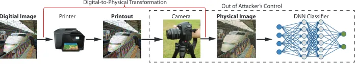
Digitial Image Printer Printout Camera Physical Image DNN Classifier Digital-to-Physical Transformation

Out of Attacker’s Control

Figure 1: Adversarial examples are transformed across the digital and physical worlds before they enter the DNN image classi-fier. In practice, attackers have no (limited) control over the internal system.

Basic Iterative Method (BIM). Basic iterative method presents a simple idea to generate adversarial noises (Good-fellow, Shlens, and Szegedy 2014). The goal is to find a small δ so that F(X+δ) =y′. The method aims to solve

the following objective function:

arg min

δ

L(F(X+δ),y′) +c· ||δ||p

where c controls the regularization of the distortion, and ||δ||pis the Lpnorm that specifies||Xadv−X||p<δ. The

optimization aims to cause a mis-classification fromytoy′

while minimizing the perturbation tox.

BIMdoes notconsider the physical world challenges. As

shown in Figure 1, it is unlikely that attackers can directly feed the generated adversarial example (a digital image) into the classifier. More practically, the digital image can be printed by the attacker as a physical object (e.g., a poster), which is then captured by the camera of the target system (e.g., a self-driving car) and digitalized into a new image (referred as “physical image”). This physical image is the actual input of the classifier. Since attackers have very lim-ited control over the internal parts of the system, the different angles to take the photo or the nonlinear response functions of the camera can affect the attack success rate.

Expectation over Transformation (EOT). The EOT method (Athalye et al. 2018) aims to improve the robust-ness of adversarial examples using a series of synthetically transformed images (in the digital domain). More specifi-cally, EOT applies a transformation functiont to generate a distributionT for noise optimization, in order to make the perturbationδ more robust to physical changes. The objec-tive function is of the form:

arg min

δ

Et∈T L(F(t(X+δ)),y′) +c· ||δ||p.

Here, transformationtcan be either image translation, rota-tion, scaling, lighting variations, and contrast changes. Note that, however,EOTis solely based on the synthesis ofdigital

images, which still ignores the physical effects introduced by the digital-to-physical transformations.

Robust Physical Perturbations (RP₂). The RP2

method (Evtimov et al. 2018) enhances the EOT method by also consideringthe physical images. TheRP2method,

however, requires the attacker to print out a clean image and take a number of photos of the printout from different angles and distances (physical images). The set of physical

images are denoted asXV.RP2solves this optimization:

arg min

δ

Et∈T,x∈XV L(F(t(x+δ)),y′) +c· ||δ||p

RP2is only tested on5road signs, and it is not yet clear

if the method is broadly applicable; More importantly, the need of manually printing and taking multiple photos for producingeachadversarial example hurts its practical value. For all the methods above, the optimization problem can be solved by stochastic gradient descent and back-propagation, provided that the classifierF is differentiable. The expectation can be approximated by empirical mean

(i.e.,Monte Carlo integration). For instance, in basic

itera-tive method,Xadvis obtained when the following optimiza-tion equaoptimiza-tions 1 converge. Note that the “clip” funcoptimiza-tion is to ensure thatXadv_{is a valid image and}_L

∞ε-neighborhood of

the clean imageX.

Xadv

N+1=XadvN +αsign(▽J(XadvN−1,y

′₎₎

Xadv_N₊₁=clip(Xadv_N₊₁,X+ε,X−ε) (1)

Defining Key Terms. We use Figure 1 to define impor-tant terms for the rest of the paper. (1) “digital image”: the original image in the digital form. (2) “printout”: the printed paper/poster of the original image. (3) “physical image”: the photograph of the printout taken by a camera.

Our Method

In this section, we present a simple yet surprisingly effec-tive method to generate robust adversarial examples in the physical world. The core idea is to explicitly simulate the physical-to-digital transformation introduced by (1) craft-ing the physical object (e.g., image printing), and (2) digi-talizing the physical object by the target system (e.g., by a camera). Our goal is to generate adversarial noises that can survive the digital-to-physical transformation in practice. In addition, our method remains simulation-based, which elim-inates the costly process of manually takingphysical images

for every single adversarial example (unlikeRP2). We call

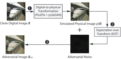
our methodD2P, short for “digital-to-physical transforma-tion”. Figure 2 shows the high-level workflow.

Step 1. We first simulate the digital-to-physical transfor-mation using a conditional Generative Adversarial Networks (cGANs) for performing image-to-image translation (Isola et al. 2017; Zhu et al. 2017).2The cGANs model has shown

2_{Other image-to-image translation models can be applied here}

(4)

Digital-to-physical Transformation (Pix2Pix / cycleGAN)

+

Expectation over

Transform (EOT) Clean Digital Image X Simulated Physical Image p(X)

Adversarial Noise Adversarial Image Xadv

1

2

3

Figure 2: We use a conditional Generative Adversarial Net-work (pix2pix or cycleGAN) to learn the digital-physical transformation for generating a synthetic physical image, which then serves as the “base” for producing adversarial noises.

successes in tasks such as labeling maps and coloring im-ages. We tailor a network to capture the transformation from a digital image to its physical version to simulate the nonlin-ear quantization effect of physical devices (e.g., cameras).

Our cGANs model is trained to learn mapping function

p:D→PwhereDis a set of images in the digital domain andP is a set of physical images (i.e., the photos of print-outs taken by a camera). We train the model using a set of paired training examples{xi}N₁ and{xV_i }N₁ wherexi∈Dand xV_i ∈P. We denote the data distribution asx∼pdata(x)and

xV∼pdata(xV)for brevity. In addition to the mapping func-tion (i.e., the generator), cGans has another component, dis-criminatorC, which aims to discriminatexV and p(x). We train the cGan models via the following objective function:

LcGANs=ExV log(CP(xV)) +Exlog(1−CP(p(x))), (2)

where the generator p tries to generate images p(x) that look similar to images xV from the physical domain P, while the discriminatorCPaims to distinguish between

sim-ulated physical image p(x)and real samplesxV. For D2P,

we consider two types of cGANs (equation 2) to improve the performance. First, pix2pix model (Isola et al. 2017) mixed it with a pixelwise reconstruction loss such asL1 or

L2 distance. Second, cycleGAN (Zhu et al. 2017) mixed it with cycle loss and learned another set of generator (p′ :

P→D) and discriminator (C′_P). The generator p′ trans-forms the simulated physical image p(X) back to digital domain and make p′(p(X))look similar to its original in-put X; Note that unlike pix2pix, cycleGAN does not re-quire “paired” images for training, which can tolerate the potential misalignment between the digital and physical im-age. We adopt the network architecture in (Isola et al. 2017; Zhu et al. 2017) and follow the training procedure for train-ing our D2P transformation network.

Step 2. After training the cGAN model, given an input digital imageX, we map the imageXto thesimulated phys-ical imagep(X). We then usep(X)as the “base” and apply the Exception over Transformation (EOT) method to gener-ate adversarial noises. By sampling the geometric transfor-mation of p(X), the EOT method can further improve the

Table 1: Similarity (SSIM) and Dis-similarity (MSE) in comparison with the original digital image, after different several times of digital-to-physical transformation.

Similarity # of Transformations

Metric 0 1 2 3 4

SSIM 1.00 0.69 0.54 0.49 0.42 MSE 0.00 1788.75 3180.50 4625.07 4852.89

robustness of the produced adversarial noise over different viewpoints. Note that our method is operated viadigital

sim-ulations, which incur a low cost. Later, we show that the

cGANs can be trained with a one-shot effort using a small set of images (e.g., 200). Once it is trained, the model gen-eralizes well to various different types of images (scalable).

Step 3. The adversarial noise is then added to the

simu-lated physical image p(X)to generate the adversarial

im-age. This is very different from existing works which add noise to the digital image X (Carlini and Wagner 2017; Athalye et al. 2018; Evtimov et al. 2018). Our design is mo-tivated by an observation from our experiments: after going through physical devices (printers, cameras), the digital im-ages would lose certain features and details due to quantiza-tion. Such physical transformation effect is the strongest for the first time and then becomes much weaker when going through multiple rounds of transformations.

Table 1 validates this observation. We randomly select 30 images from the ImageNet validation dataset (Russakovsky et al. 2014). For each image, we print it out using a printer and retake the photo of the printout using a camera at the frontal view. We consider as one round of digital-to-physical transformation. We then perform multiple rounds of transformation and measure the image similarity (or dis-similarity) to the original clean image. As shown in Table 1, we use the Structural Similarity Index (SSIM) (Wang et al. 2004) and Mean Squared Error (MSE) as the similarity met-ric. Our results validate that the loss is more significant dur-ing the first round, and then becomes much smaller for the third and fourth round. The result suggests that if we use a (simulated) physical image as the base, the resulting ad-versarial example is more likely to survive another round of quantization during the attack.

Experimental Evaluation

We evaluate the effectiveness of adversarial examples in the physical domain with two goals. First, we seek to compare our method with the state-of-the-art over a much

larger-scalephysical domain measurements. Over different

exper-iment settings, we printed and shot over 3000 physical im-ages for a comprehensive evaluation. Second, we seek to ex-amine the transferability of our method,i.e., how well an adversarial example optimized for a specific DNN classifier and a pretrained pix2pix/cycleGAN model can transfer to other classifiers, cameras, and printers.

(5)

Clean Image BIM EOT RP2 Our D2Pp Our D2Pc

Figure 3: Adversarial examples in the physical domain. The targeted attack aims to make the classifier mis-classify the input image from the original label “king penguin” to the target label “kite”.

Table 2: Similarity between the real physical image and the simulated physical image using pix2pix.

Training Size 50 100 150 200 250 300 SSIM 0.37 0.40 0.44 0.45 0.45 0.46 Perception Loss 0.44 0.41 0.40 0.38 0.38 0.37

advanced EOT and RP2 methods. We choose the widely

used Inception-V3 (Szegedy et al. 2016) as thetarget

clas-sifier, which is pre-trained from the ImageNet dataset

(Rus-sakovsky et al. 2014). Note that the “physical experiments” require us manually printing images and taking photos, which cannot be fully automated to reach a large scale. To this end, we randomly sampled 102 images (96 classes) from the ImageNet’s validation set (50000 images) (Russakovsky et al. 2014) as ourExp Dataset.

For our D2P method, we trained two types of cGANs to model the digital-to-physical transformation: one is pix2pix (referred as D2Pp), and the other one is cycleGAN (referred

as D2Pc). We use 200 training images randomly selected

from ImageNet’s validation set. To build the ground-truth, we print each image and then re-take the photo to obtain its physical version (Canon PIXMA TS9020 printer and iPhone 6s camera), and use this dataset with paired digital and phys-ical images to facilitate the training. These 200 imageshave

no overlapwith the 102 images in theExp Dataset. In this

way, we can test whether cGANs is indeed generalizable to unseen images. For applying the EOT method, we follow a standard configuration, and considerscaling(from 0.5 to 2.0),rotation(from−45◦to 45◦) andtranslation(from -0.2 to 0.2). The parameters are uniformly sampled.

We only use 200 images for training because our prelimi-nary experiment shows a small training dataset is sufficient. For brevity, we use pix2pix model to demonstrate the impact of training data size (results are similar for cycleGAN). Ta-ble 2 shows how the size of training dataset affects the qual-ity of the pix2pix output. More specifically, we measure the similarity between the actual physical images and the simu-lated physical images produced by the pix2pix model based on SSIM and Perception Loss (Richard Zhang 2018). The similarity scores hit diminishing returns after 200 images. Even though training is a one-shot effort, it is desirable to reduce the manual efforts to produce training data.

We performtargeted attacksfor all cases. For a given in-put image, we use the proposed attack method to generate adversarial noises aiming to misclassify the image as the

least-likelylabel (a more difficult attack). For example,

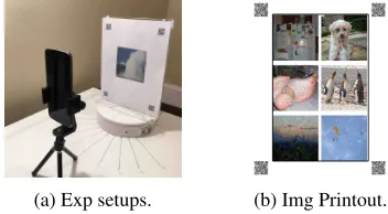
sup-(a) Exp setups. (b) Img Printout.

Figure 4: (a) Exp setups. (b) Img printout.

pose an input has a true label of “dung beetle”, the “most-likely” label is the label that has the second highest clas-sification probability, which is “ground beetle”. The “least-likely” label is the one with the lowest probability: “Ameri-can lobster”. Clearly, it is more challenging to cause a mis-classification to the least-likely label. For all the methods, if not otherwise stated, we set the step sizeα=0.5 and noise levelε=30 to maintain the same level of adversarial noises.

As shown in Figure 3, the adversarial examples are still vi-sually recognizable as the original label (“King penguin”), but will be misclassified to the target label (“Kite”).

Experiment Process. Given a digital imageX, the exper-iment process is the following. First, We use the proposed D2P model to generate a simulated physical image p(X)as a base image. Second, we add the adversarial noise to this base image. Third, we print the new image out on a paper as a printout. Fourth, we take a photo of the printout using a phone. Fifth, we send this photo to a DNN classifier, and evaluate the attack performance.

For our baseline methods (BIM, EOT,RP2), we follow the

same process except for the first step. Instead of using the simulated physical image p(X) as a base, we directly use the clean imageXas their base image.

(6)

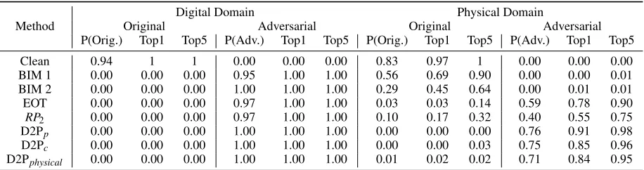
Table 3: Classification confidence and accuracy of adversarial examples. BIM 1’s noise level (ε=30,α=0.5) is the same with

all other methods. BIM 2 uses bigger noises (ε=70,α=0.5).

Digital Domain Physical Domain

Method Original Adversarial Original Adversarial P(Orig.) Top1 Top5 P(Adv.) Top1 Top5 P(Orig.) Top1 Top5 P(Adv.) Top1 Top5 Clean 0.94 1 1 0.00 0.00 0.00 0.83 0.97 1 0.00 0.00 0.00 BIM 1 0.00 0.00 0.00 0.95 1.00 1.00 0.56 0.69 0.90 0.00 0.00 0.01 BIM 2 0.00 0.00 0.00 1.00 1.00 1.00 0.29 0.45 0.64 0.00 0.01 0.01 EOT 0.00 0.00 0.00 0.97 1.00 1.00 0.03 0.03 0.14 0.59 0.78 0.90

RP2 0.00 0.00 0.00 0.97 1.00 1.00 0.10 0.17 0.32 0.40 0.55 0.75

D2Pp 0.00 0.00 0.00 1.00 1.00 1.00 0.00 0.00 0.00 0.76 0.91 0.98 D2Pc 0.00 0.00 0.00 1.00 1.00 1.00 0.00 0.00 0.03 0.75 0.85 0.96 D2Pphysical 0.00 0.00 0.00 1.00 1.00 1.00 0.01 0.02 0.02 0.71 0.84 0.95

measured accurately. All photos are taken under the normal indoor lighting. By default, we use a Canon PIXMA TS9020 printer and the iPhone 6s camera. Later, we will examine the transferability using a different printer and camera.

Exp A: Effectiveness of Adversarial Examples

We start with the “frontal view” and examine how likely the adversarial examples can fool the classifier. Table 3 shows three key evaluation metrics. First, we report the probability (i.e., confidence) produced by the classifier which indicates the likelihood of the input to be classified as each label. We show the average confidence of the original label (P(Orig.)) and that of the target label (P(Adv.)). Second, after ranking the labels based on the confidence, we show the percentage of images whose original label is ranked top-1 and top-5. Third, we also show how likely the target label is ranked at the top-1 and top-5. In Table 3, the “’clean” row refers to clean images without attacks. The classifier has a perfect classification accuracy (100%) in the digital domain and a near-perfect performance in the physical domain. A success-ful adversarial example will suppress the original label (low

P(Orig.) — low top-1 and top-5 ratio for the original label), and promote the target label (highP(Adv.) — high top-1 and top-5 ratio for the target label).

We have four key observations from the attack results. First, as shown in the left half of the table, the digital ver-sions of the adversarial images are highly successful. Across all the methods, 100% of the original labels are dropped out of 5, and the target label is always classified as the top-1. This shows that in the digital domain, a classifier can be extremely vulnerable to adversarial attacks.

Second, as shown in the right half of the table, adver-sarial examples are more difficult to succeed in the physi-cal domain. The top-1 accuracy of the target label dropped significantly for BIM to 0.00 and 0.01. The results suggest that the basic methods do not work in the physical domain. Advanced methods such as EOT andRP2have a better

per-formance, which confirms the advantage of optimizing over simulated geometric transformations.

Third, both of our D2P models outperform existing meth-ods by a large margin. Compared to EOT and RP2, our

method significantly improves the target label’s ranking. For example, using D2Pp, the top-1 accuracy of the target label

is improved to 0.91 from 0.55 and 0.78. The top-5

accu-racy of the target label is improved to 0.98. In addition, our method successfully reduces the original label’s top-1 and top-5 accuracy to 0. These results demonstrate the benefits of using asimulated physical image as the base to gener-ate adversarial examples and the cGANs have successfully captured the patterns of D2P transformation.

Fourth, D2Ppslightly outperforms D2Pcin the attacking

results. D2Pc uses the cycleGAN for learning the

digital-to-physical transformation. The simulated physical images are more authentic compared with the real physical images because the training does not suffer from potential misalign-ment between the digital and physical images. As evidence, we measure the average Perception Loss, a metric to assess the visual dissimilarity (Richard Zhang 2018) between the actual physical image and the simulated one. We find that cycleGAN indeed has a lower loss (0.28) than the pix2pix model (0.38). Although cycleGAN makes the generated im-age more faithful to the real physical imim-age (see the example in Figure 3), it also preserves more features of the original image which makes the attack more difficult. The attacking performance of D2Pcis slightly weaker than that of D2Pp.

Given the good performance of D2P, a natural question is whether the performance would be even better if we directly use the physical image as the base (D2Pphysical). This

rep-resents the best base image that the D2P model can output. As shown in Table 3, the result is counter-intuitive, as D2Pc

and D2Ppperform slightly better than D2Pphysical. A

possi-ble explanation is that the performance gain may come from the feature loss during the quantization. The simulated phys-ical images produced from the cGAN model exhibit slight distortions compared to the corresponding physical images. The feature loss makes the simulated images slightly easier to attack. In the rest of the paper, we use D2Ppto examine

the robustness of adversarial examples.

Exp B: Robustness against Viewing Angles

(7)

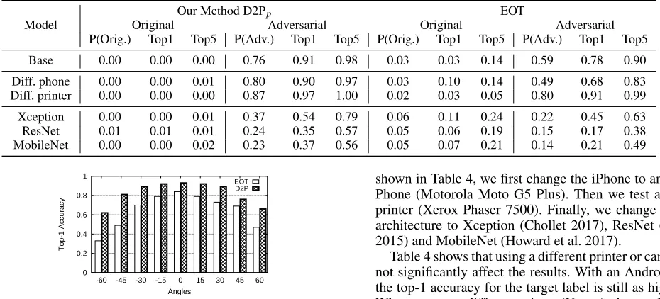
pho-Table 4: Transferability of adversarial examples. “Base” represents the result of the original configuration of Exp. A and B. We then examine the performance of adversarial examples under different phone cameras, printers, and classifiers.

Our Method D2Pp EOT

Model Original Adversarial Original Adversarial P(Orig.) Top1 Top5 P(Adv.) Top1 Top5 P(Orig.) Top1 Top5 P(Adv.) Top1 Top5 Base 0.00 0.00 0.00 0.76 0.91 0.98 0.03 0.03 0.14 0.59 0.78 0.90 Diff. phone 0.00 0.00 0.01 0.80 0.90 0.97 0.03 0.10 0.14 0.49 0.68 0.83 Diff. printer 0.00 0.00 0.00 0.87 0.97 1.00 0.02 0.03 0.05 0.80 0.91 0.99 Xception 0.00 0.00 0.01 0.37 0.54 0.79 0.06 0.11 0.24 0.22 0.45 0.63 ResNet 0.01 0.01 0.01 0.24 0.35 0.57 0.05 0.06 0.19 0.15 0.17 0.38 MobileNet 0.00 0.00 0.02 0.23 0.37 0.56 0.05 0.07 0.21 0.14 0.21 0.49

0 0.2 0.4 0.6 0.8 1

-60 -45 -30 -15 0 15 30 45 60

Top-1 Accuracy

Angles

EOT D2P

Figure 5: Top-1 accuracy of target label for the adversarial examples under different viewing angles.

tos. To accurately capture the angle, we print one image at a time (instead of 6 images per paper). For this experiment, we only compare our D2Ppmethod with the best performing

baseline, the EOT method (ε=30).

Figure 5 shows that both methods perform reasonably well under different angles. This is largely benefited from the syntheticgeometric transformationsused by both meth-ods. Our D2P method has a better performance compared to EOT, and the advantage is more significant at larger an-gles. For example, at the frontal view, our top-1 accuracy is 0.91 and EOT’s is 0.78. When the image is turned by 45 degrees, our method still has a top-1 accuracy of 0.62 while the accuracy of EOT degrades to 0.33. The results confirm the robustness of our adversarial examples. Recall that our digital-to-physical model was trained only using the

front viewimages. The result shows that the transformation

helps to generalize better the attack effectiveness (compared to EOT) to other previouslyunseensituations (i.e., images captured from different view angles).

Exp C: Transferability of Adversarial Examples

Finally, we validate the transferability of the proposed adver-sarial examples. So far, we were using a specific DNN model (Inception-V3), camera (iPhone 6S), and printer (Canon PIXMA TS9020) to generate adversarial examples. Below, we examine how robust these adversarial examples are when we (1) print the adversarial images with a different printer; (2) take photos with a different camera, and (3) classify the physical images with a different classifier. This simulates a practical scenario where the attacker does not have full knowledge of the target system. all adversarial examples are generated in the same setting as before (Inception V3). Next, we test the images by changing one condition at a time. As

shown in Table 4, we first change the iPhone to an Android Phone (Motorola Moto G5 Plus). Then we test a different printer (Xerox Phaser 7500). Finally, we change the DNN architecture to Xception (Chollet 2017), ResNet (He et al. 2015) and MobileNet (Howard et al. 2017).

Table 4 shows that using a different printer or camera does not significantly affect the results. With an Android phone, the top-1 accuracy for the target label is still as high as 0.9. When we use a different printer (Xerox), the result actually gets better (top-1 accuracy is 0.97). We believe that this is because the Xerox printer is a laser printer with a higher DPI (1600). The Canon printer used to train the pix2pix net-work is an ink printer with 600 DPI. Therefore, the quanti-zation effect has been over-estimated during training, and the performance improves when the adversarial examples are printed out by a high-DPI printer.

The DNN architecture, however, does have an impact. We observe that Xception performs better than ResNet and Mo-bileNet, which is likely due to the fact that Xception uses the same image size (299×299) as the original Inception-V3, while the other two would reshape the images before clas-sification. We suspect the digital-to-physical transformation also plays a role. To validate this hypothesis, we performed an experiment where we directly feed the digital version

of the adversarial images into the target classifiers. We ob-serve the performance degradation is much smaller on digi-tal images. Consistently across all settings, we show that our method has a better transferability compared with EOT. This indicates that our cGANs model has captured generalizable characteristics of the physical domain transformation.

Discussion and Conclusion

In this paper, we explore the feasibility of generating ro-bust adversarial examples that can survive in the physical world. We propose the D2P method to simulate the com-plex effect introduced by physical devices to construct more robust adversarial examples. Our results show that the sim-ulated transformation helps improve the attack effectiveness to otherunseenoruncontrolledsituations such as different viewing angles, printers, and cameras.

(8)

applications, such as object detection systems used by self-driving cars and home-security systems; (2) improving fense methods against adversarial examples. So far, most de-fense methods are designed to detectdigital-domain adver-sarial noises (Papernot et al. 2017). Using D2P, we can gen-erate morerealisticadversarial examples to assist the trou-bleshooting of under-trained regions and augment the train-ing data for model retraintrain-ing (Rozsa, Rudd, and Boult 2016) or adversary detection (Xu, Evans, and Qi 2018). By adding our adversarial examples into the training data, we expect the re-trained classifier to be more robust against attacks.

Acknowledgments

This work is supported by NSF grant CNS1750101 and CNS-1717028.

References

Athalye, A.; Engstrom, L.; Ilyas, A.; and Kwok, K. 2018. Synthe-sizing robust adversarial examples. InProc. of ICML.

Bastani, O.; Ioannou, Y.; Lampropoulos, L.; Vytiniotis, D.; Nori, A. V.; and Criminisi, A. 2016. Measuring neural net robustness with constraints. InProc. of NIPS.

Brown, T. B.; Man´e, D.; Roy, A.; Abadi, M.; and Gilmer, J. 2017. Adversarial patch.CoRRabs/1712.09665.

Carlini, N., and Wagner, D. A. 2017. Towards evaluating the ro-bustness of neural networks. InProc. of IEEE S&P.

Chen, Q., and Koltun, V. 2017. Photographic image synthesis with cascaded refinement networks. InProc. of ICCV.

Chollet, F. 2017. Xception: Deep learning with depthwise separa-ble convolutions. InProc. of CVPR.

Cisse, M.; Adi, Y.; Neverova, N.; and Keshet, J. 2017. Houdini: Fooling deep structured visual and speech recognition models with adversarial examples. InProc. of NIPS.

Evtimov, I.; Eykholt, K.; Fernandes, E.; Kohno, T.; Li, B.; Prakash, A.; Rahmati, A.; and Song, D. 2018. Robust physical-world attacks on machine learning models. InProc. of CVPR.

Eykholt, K.; Evtimov, I.; Fernandes, E.; Li, B.; Song, D.; Kohno, T.; Rahmati, A.; Prakash, A.; and Tram`er, F. 2017. Note on attacking object detectors with adversarial stickers. CoRR

abs/1712.08062.

Fischer, V.; Chaithanya Kumar, M.; Hendrik Metzen, J.; and Brox, T. 2017. Adversarial examples for semantic image segmentation.

CoRRabs/1707.08945.

Fonseca, F., and Krisher, T. 2018. Uber suspends self-driving car tests after pedestrian death in arizona. Chicago Tribune.

Goodfellow, I.; Shlens, J.; and Szegedy, C. 2014. Explaining and Harnessing Adversarial Examples. InProc. of ICLR.

He, K.; Zhang, X.; Ren, S.; and Sun, J. 2015. Deep residual learn-ing for image recognition.CoRRabs/1512.03385.

Howard, A. G.; Zhu, M.; Chen, B.; Kalenichenko, D.; Wang, W.; Weyand, T.; Andreetto, M.; and Adam, H. 2017. Mobilenets: Effi-cient convolutional neural networks for mobile vision applications.

CoRRabs/1704.04861.

Huang, S. H.; Papernot, N.; Goodfellow, I. J.; Duan, Y.; and Abbeel, P. 2017. Adversarial attacks on neural network policies. InProc. of ICLR Workshop.

Isola, P.; Zhu, J.-Y.; Zhou, T.; and Efros, A. A. 2017. Image-to-image translation with conditional adversarial networks. InProc. of CVPR.

Kos, J., and Song, D. 2017. Delving into adversarial attacks on deep policies. InProc. of ICLR Workshop.

Kurakin, A.; Goodfellow, I. J.; and Bengio, S. 2017. Adversarial examples in the physical world. InProc. of ICLR Workshop. Lin, Y.; Hong, Z.; Liao, Y.; Shih, M.; Liu, M.; and Sun, M. 2017. Tactics of adversarial attack on deep reinforcement learning agents. InProc. of IJCAI.

Lu, J.; Sibai, H.; Fabry, E.; and Forsyth, D. A. 2017. NO Need to Worry about Adversarial Examples in Object Detection in Au-tonomous Vehicles. InCVPR Workshop.

Lu, J.; Sibai, H.; and Fabry, E. 2017. Adversarial examples that fool detectors.CoRRabs/1712.02494.

Moosavi-Dezfooli, S.; Fawzi, A.; and Frossard, P. 2016. Deepfool: A simple and accurate method to fool deep neural networks. In

Proc. of CVPR.

Papernot, N.; McDaniel, P. D.; Jha, S.; Fredrikson, M.; Celik, Z. B.; and Swami, A. 2016. The limitations of deep learning in adversar-ial settings.Proc. of IEEE Euro. S&P.

Papernot, N.; McDaniel, P.; Goodfellow, I.; Jha, S.; Celik, Z. B.; and Swami, A. 2017. Practical black-box attacks against machine learning. InProc. ASIA CCS.

Richard Zhang, Phillip Isola, A. A. E. E. S. O. W. 2018. The unreasonable effectiveness of deep features as a perceptual metric. InProc. of CVPR.

Rozsa, A.; Rudd, E. M.; and Boult, T. E. 2016. Adversarial diver-sity and hard positive generation. InProc. of CVPR Workshop. Russakovsky, O.; Deng, J.; Su, H.; Krause, J.; Satheesh, S.; Ma, S.; Huang, Z.; Karpathy, A.; Khosla, A.; Bernstein, M. S.; Berg, A. C.; and Li, F. 2014. Imagenet large scale visual recognition challenge.

CoRRabs/1409.0575.

Sharif, M.; Bhagavatula, S.; Bauer, L.; and Reiter, M. K. 2016. Accessorize to a crime: Real and stealthy attacks on state-of-the-art face recognition. InProc. of CCS.

Sitawarin, C.; Bhagoji, A. N.; Mosenia, A.; Chiang, M.; and Mittal, P. 2018. DARTS: deceiving autonomous cars with toxic signs.

CoRRabs/1802.06430.

Szegedy, C.; Zaremba, W.; Sutskever, I.; Bruna, J.; Erhan, D.; Goodfellow, I.; and Fergus, R. 2014. Intriguing properties of neural networks. InProc. of ICLR.

Szegedy, C.; Vanhoucke, V.; Ioffe, S.; Shlens, J.; and Wojna, Z. 2016. Rethinking the inception architecture for computer vision. InProc. of CVPR.

Wang, Z.; Bovik, A. C.; Sheikh, H. R.; and Simoncelli, E. P. 2004. Image quality assessment: From error visibility to structural simi-larity.IEEE TIP13(4).

Wang, T.-C.; Liu, M.-Y.; Zhu, J.-Y.; Tao, A.; Kautz, J.; and Catan-zaro, B. 2018. High-resolution image synthesis and semantic ma-nipulation with conditional gans. InProc. of CVPR.

Xie, C.; Wang, J.; Zhang, Z.; Zhou, Y.; Xie, L.; and Yuille, A. 2017. Adversarial examples for semantic segmentation and object detec-tion. InProc. of ICCV.