Applying nonlinear MODM model to supply chain management with quantity discount policy under complex fuzzy environment

JIEM, 2014 – 7(3): 660-680 – Online ISSN: 2013-0953 – Print ISSN: 2013-8423 http://dx.doi.org/10.3926/jiem.1079

Applying Nonlinear MODM Model to Supply Chain Management with

Quantity Discount Policy under Complex Fuzzy Environment

Zhe Zhang

1

, Jiuping Xu

2

*

1

School Economics & Management, Nanjing University of Science and Technology (CHINA)

2

Uncertainty Decision-Making Laboratory, Sichuan University (CHINA)

[email protected], [email protected]

Received: January 2014

Accepted: May 2014

Abstract:

Purpose:

The aim of this paper is to deal with the supply chain management (SCM) with

quantity discount policy under the complex fuzzy environment, which is characterized as the

fuzzy variables. By taking into account the strategy and the process of decision making, a

bi-fuzzy nonlinear multiple objective decision making (MODM) model is presented to solve the

proposed problem.

Design/methodology/approach:

The bi-fuzzy variables in the MODM model are

transformed into the trapezoidal fuzzy variables by the DMs's degree of optimism

α

1

and

α

2

,

which are de-fuzzified by the expected value index subsequently. For solving the complex

nonlinear model, a multi-objective adaptive particle swarm optimization algorithm (MO-APSO)

is designed as the solution method.

Findings:

The proposed model and algorithm are applied to a typical example of SCM

problem to illustrate the effectiveness. Based on the sensitivity analysis of the results, the

bi-fuzzy nonlinear MODM SCM model is proved to be sensitive to the possibility level

α

1

.

Originality/value:

The bi-fuzzy variable is employed in the nonlinear MODM model of SCM

to characterize the hybrid uncertain environment, and this work is original. In addition, the

hybrid crisp approach is proposed to transferred to model to an equivalent crisp one by the

DMs's degree of optimism and the expected value index. Since the MODM model consider the

bi-fuzzy environment and quantity discount policy, so this paper has a great practical

significance.

Keywords:

bi-fuzzy variable, nonlinear, multi-objective programming, sensitivity analysis, particle

swarm optimization

1. Introduction

The remainder of this paper is organized as follows. In section 2, some preliminaries about the bi-fuzzy theory are presented. Then a bi-fuzzy nonlinear MODM SCM model with quantity discount policy is proposed in section 3. The details of an approach used in transforming bi-fuzzy variables into the bi-fuzzy variables are also presented, and then the expected value operator is employed to deal with the fuzzy variables. In section 4, a multi-objective adaptive particle swarm optimization algorithm (MOBL-APSO) is utilized to resolve the nonlinear MODM model. The effectiveness of the proposed model and algorithm is proven by the practical application in section 5. Finally, in section 6, concluding remarks and further research are outlined.

2. Preliminaries

Some basic knowledge of fuzzy set theory, bi-fuzzy variable and bi-fuzzy MODM model will be introduced in this section.

Definition 2.1. (Zadeh, 1965) Given a domain X. If à is a fuzzy subset of X, for any x

ϵ

X

μÃ: X → [0,1], x → μÃ(x)

μà is named a membership function of x with respect to Ã. μÃ(x) denotes the grade to each point in X with a real number in the interval [0,1] that represents the grade of membership of

x in A. à is a fuzzy set and described as à = {(x, μÃ(x))|x

ϵ

X}. If F is a fuzzy number (set) with degree of membership μF(u) of an element u in F, then μF(u) represents the degree of possibility that a parameter x has a value u. Thus, the nearer the value of μÃ(x) is unity, the higher the grade of membership of x in Ã.

Definition 2.2. (Zadeh, 1978) Let à be a fuzzy set which defined on X. If

α

is possibility level

and 0 ≤

α

≤ 1, Ãα consist of all elements whose degrees of membership in à are greater than

or equal to

α

,

Ãα = {x

ϵ

X|μÃ(x) ≥ a}

then Ãα is called the

α

-level set of fuzzy set Ã.

Definition 2.3. (Dubois & Prade, 1988) Let

Θ

be a nonempty set, P(

Θ

)

be the power set of

Θ

,

Definition 2.4. (Nahmias, 1978) A fuzzy variable is a function from a possibility space (

Θ

,

P(

Θ

)

, Pos) to the real line R.

Definition 2.5. (Liu, 2002) A bi-fuzzy variable is a function from a possibility space (

Θ

, P(

Θ

)

, Pos) to a collection of fuzzy variables.

Roughly speaking, a bi-fuzzy variable is a fuzzy variable defined on the universal set of fuzzy

variables. For example, let , where is a fuzzy variable with membership function

. Then is a bi-fuzzy variable obviously (Liu, 2002).

Based on the definitions above, the bi-fuzzy MODM model can be stated as:

(1)

Where are bi-fuzzy vectors,

and b = (b1, b2, ···, bm)T.

Definition 2.6. (Luhandjula, 1987) Let be the possibility level vector,

, x

ϵ

Rn_{, and if}

then x is

α

1-possible feasible solution to (1). All

α

1-possible feasible solutions are

α

1-possible

feasible set of the model (1).

Consider the form of model (1) as:

(2)

Then, let

α

2 be a possibility level,

α

2

ϵ

[0,1], D

ϵ

Rn, and x '

ϵ

D. If do not exist x

ϵ

D and

k

ϵ

1,2, ···, K, x satisfy

x' is

α

2-possible

Definition 2.7. (Luhandjula, 1987) Let x'

ϵ

X, if x' is the problem

(3)

α

1-possible efficient solution, and then x' is (

α

1,

α

2)-satisfied solution of the model (1).

Actually, in order to solve model (1) and find the (

α

1,

α

2)-satisfied solution, the following MODM

model should be considered:

(4)

Where is

α

1-level set of bifuzzy variables .

Theorem 1. (Xu & Liu, 2008) x' is the (

α

1,

α

2)-satisfied solution of the model (1) if and only if

x' is the efficient solution of the model (4).

3. Bi-fuzzy non-linear MODM model for SCM

Traditionally, there are three stages in the supply chain, including procurement, production and distribution. The general structure of a typical supply chain is outlined in Figure 1. For simplifying the presentation, only the manufacturers, distribution centers, and retailers are considered in this paper.

Figure 1. The schema of supply chain

V e n d o r

V e n d o r

M a n u f a c t u r e r

M a n u f a c t u r e r

C u s t o m e r

C u s t o m e r

C u s t o m e r D i s t r i b u t i o n

c e n t e r

D i s t r i b u t i o n c e n t e r

D i s t r i b u t i o n c e n t e r

R e t a i l e r

3.1. Modelling

Since treating the nonlinear functions is difficult, some SCM models assume that the prices of materials, production, inventory, and transportation are constant. However, this assumption is far beyond the practical situation. The vendors usually offer quantity discounts to encourage the buyers to order more, and the producer intends to discount the unit production cost if the amount of production is large. In this case, the quantity discount policy should be considered.

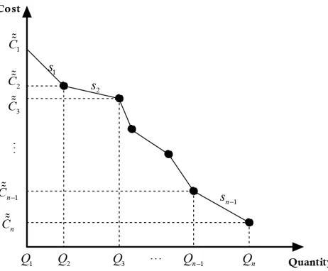
Note that the cost (price) variables can be expressed as a function of quantity Q, and the multiple breakpoint discount function is a general form usable in practice (see Figure 2). The function can be represented as:

(5)

where si is the slope when the quantity ordered is between Qi and Qi+1, and n means that there

are n-1 line segments in .

Figure 2. Multiple breakpoint discount function

3.1.1. Notion

: Ordered quantity of the pth product from the mth manufacturer in the tth period

: Quantity of the pth product transported from the mth manufacturer to the dth distribution center in the tth period

: Quantity of the pth product in the dth distribution center in the tth period

: Quantity of the pth product transported from the dth distribution center to the rth retailer in the tth period

: Unit procurement cost of the pth product from the mth manufacturer in the tth period

: Unit transportation cost of the pth product from the mth manufacturer to the dth distribution center in the tth period

: Unit transportation cost of the pth product from the dth distribution center to the rth retailer in the tth period

: Unit stock carrying cost of the pth product in the dth distribution center in the tth period

: Short safe inventory level in the mth manufacturer, dth distribution center, rth retailer in the tth period

: Safe inventory quantity in the mth manufacturer, dth distribution center, rth retailer in the tth period

: Inventory level of the pth product in the mth manufacturer, dth distribution center, rth retailer in the tth period

: Maximum inventory capacity of the mth manufacturer, dth distribution center, rth retailer

: Lead time from the mth manufacturer to the dth distribution center and LTmd ≤ T

: Lead time from the dth distribution center to the rth retailer and LTdr ≤ T

: Maximum supplied level of the pth product from the mth manufacturer in the tth period

3.1.2. Model Formulation

Based on the requirement of the DM's objectives, we will develop a bi-fuzzy non-linear MODM model for SCM as follows.

3.1.2.1. Objective functions

The first objective is to minimize the total cost, which includes procurement cost, transportation cost, and inventory cost. Basically, there are four kinds of costs involved in this model: product procurement cost from manufacturers, transportation cost from manufacturers to distribution centers, inventory cost in distribution centers, and transportation cost from distribution centers to retailers. So the total cost can be described as:

(6)

Where , , , are bi-fuzzy variables.

Furthermore, the second objective is to maximize the average safe inventory levels. The safe inventory level of the mth manufacturer in the tth period is defined as the expected average percentage of 1 less the ratio of short safe inventory level of product p of manufacturer m at period t (Dt_{mp), over the safe inventory quantity of product p of manufacturer m (SImp). Similar} definitions are also applied to distribution centers and retailers. So we develop all the participants' safe inventory levels as:

(7)

3.1.2.2. Constraints

Since the amount of the pth product transported from the mth manufacturer to all distribution centers must be equal to the total amount ordered from the mth manufacturer in the tth period for each manufacturer, so

(8)

(9)

The total amount of the pth product shipped from distribution centers to retailers must be equal to the total final demands in the tth period, hence:

(10)

The maximum supplied quantity of manufacturers and inventory level of distribution centers are given:

(11)

By making the short safe inventory level of a product to be zero if inventory level is greater than safe inventory quantity, or to be the difference of safe inventory quantity and inventory level if inventory level is smaller than safe inventory quantity, here:

(12)

Based on the discussion above, by integrating the Equations (6) ~ (12), a bi-fuzzy nonlinear MODM model for SCM is developed as:

(13)

3.2. Dealing with the bi-fuzzy variable

Since some bi-fuzzy variables are involved in the proposed MODM model (13), and the costs and the quantity discount functions are variable, so it is very hard to be solved. In this case, considering the optimistic-pessimistic attitude of DMs, a hybrid crisp approach is employed to transfer the bi-fuzzy model to an equivalent one. This method transforms the bi-fuzzy variable

into a (

α

1,

α

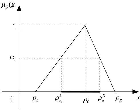
2)-level trapezoidal fuzzy variable at first, and then de-fuzzified the trapezoidal

Denoted the bi-fuzzy variable as , where is a triangular fuzzy variable

with membership function (See Figure 3).

Figure 3. The membership function of

Following the definition 2.2,

α

1-level sets of are:

where and . The parameter

α

1

ϵ

[0,1] here reflects

decision-maker's degree of optimism. In addition, can be estimated by collected data and professional experience using statistical methods.

Thus, the bi-fuzzy variable is transferred as a class of triangular fuzzy numbers,

see Figure 4. Subsequently, for the given possibility level

α

2, we can get the

α

2-level set of

these triangular fuzzy numbers as Figure 5.

Figure 4. Step 1. Transfer the bi-fuzzy variable to a class of triangular fuzzy numbers

Figure 5. Step 2. Transfer the bi-fuzzy variable to a trapezoidal fuzzy number

x

1



()

x







0



1

L





0

1

R





L





R

From Figure 5, we can see that the bi-fuzzy variable is transferred as a trapezoidal fuzzy

variables , where

Finally, a new measure with an optimistic-pessimistic adjustment index Me, which is proposed by Xu and Zhou (2011) for dealing with the trapezoidal fuzzy variable, is employed. The measure Me can evaluate a confidence degree that a fuzzy variable takes values in an interval, and the expected value of the trapezoidal fuzzy variable can be obtained by Me as (Xu & Zhou, 2011):

where λ is the optimistic-pessimistic index of DMs, and λ = 1 indicates that the best case has the maximal chance to happen, while λ = 0 is opposite.

Based on the above hybrid method, the bi-fuzzy MODM model (13) can be transformed into an equivalent crisp one.

4. Multiple Objective Adaptive PSO (MO-APSO)

Since model (13) are nonlinear, so a multi-objective adaptive particle swarm optimization algorithm (MO-APSO) is designed as the solution method. Particle swarm optimization (PSO) algorithm, which was first proposed by Kennedy and Eberhart in 1995, is an effective tool in solving optimization problems because of the superior search performance and fast convergence. PSO simulates the social behaviors such as birds flocking to a promising position for certain objectives in a multi-dimensional space (Kennedy & Eberhart, 2001). In PSO, an n-dimensional position of a particle represents a solution, and the particles fly through the problem space following the current optimum particles. The updating mechanism of particle is:

where

ν

ld(

τ

+ 1) is the velocity of l particle at the d dimension in the

τ

iteration, w is an inertia

weight, pld(

τ

) is the position of l particle at the d dimension, r1 and r2 are random numbers in

the range [0,1], cp a n d cg are personal and global best position acceleration constant respectively, meanwhile, and are personal and global best position of l particle at the d dimension.

(Coello & Lechuga, 2002). Some papers reported in the literature have extend PSO to multi-objective problems, such as Garg and Sharma (2013), Tavakkoli-Moghaddam, Azarkish and Sadeghnejad-Barkousaraie (2011), Zhang , Shao, Li and Gao (2009), and so on. The improved PSO utilizes Pareto dominance to determine the flight direction and maintains previously found non-dominated vectors in a global repository (Coello & Lechuga, 2002). All the particles are compared with each other and the non-dominated particles are stored in the repository. The position of particle is updated by:

here, REPh(

τ

) is the positions of the particles that represent non-dominated vectors in the repository, i.e., several equally good non-dominated solutions stored in the external repository instead of global best position.

The solution approach proposed in this paper combines multi-objective PSO with Pareto archived evolution strategy (PAES), which is one of Pareto-based approaches to update the best position (Knowles & Corne, 2000). This approach employs a truncated archive, which is used to separate the objective space into a number of hypercubes, to store the elite individuals. Based on the density, every hypercube has its own score. After selecting the best for particles based on roulette wheel selection, the particle is selected uniformly. More details of PAES are as:

PAES Procedure

generate initial random solution Pl(τ) and add it to the archive

update Pl(τ) to generate Pl(τ + 1)

if Pl(τ) dominates Pl(τ + 1)

discard Pl(τ + 1)

else if Pl(τ + 1) dominates Pl(τ)

replace Pl(τ) with Pl(τ + 1) and add Pl(τ + 1) to the archive

else if Pl(τ + 1) is dominated by any member in the archive

discard Pl(τ + 1)

else if Pl(τ + 1) dominates any member in the archive

replace it with Pl(τ + 1)

else if

the archive is not full add Pl(τ + 1) to the archive

if Pl(τ + 1) is in a less crowded region than Pl(τ) in the archive

accept Pl(τ + 1) as the new current solution

else

maintain Pl(τ) as the current solution

add Pl(τ + 1) to the archive, and remove a member of the archive from the

most crowded region

if Pl(τ + 1) is in a less crowed region than Plbest(τ)

accept Pl(τ) as the new current solution

else

maintain Pl(τ) as the current solution

else

do not add Pl(τ + 1) to the archive

until the termination criterion is reached, otherwise return to line 2

In addition, based on PAES, in the updating mechanism, (Shi &

Eberhart, 1998). The overall procedure of MO-APSO is presented in Figure 6.

5. Application

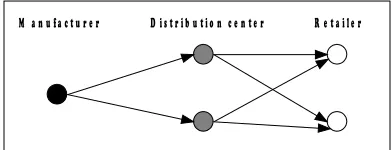
A practical supply chain application problem with quantity discount policy is considered in this section. Considering a small-scale but typical supply chain, which consists of two manufacturers (m1, m2, i.e., m = 2), two distribution centers (d1, d2, i.e., d = 2), two retailers

(r1, r2, i.e., r = 2), and two products (p1, p2, i.e., p = 2), the time period is 3 (i.e., t = 3). In

this supply chain system, the first distribution center (d1), which is small scale but fast delivery

service, can rapidly respond to the customer demand, but it also needs a high operational cost. Meanwhile, the second distribution center (d2), which is large scale but slow delivery service,

but its operational cost is low because it can use the economies of scale to transport goods. The lead-time from each manufacturer to distribution center is 1, and from distribution center to each retailer be 0. The example of supply chain is depicted in Figure 7.

Figure 7. The example of typical supply chain

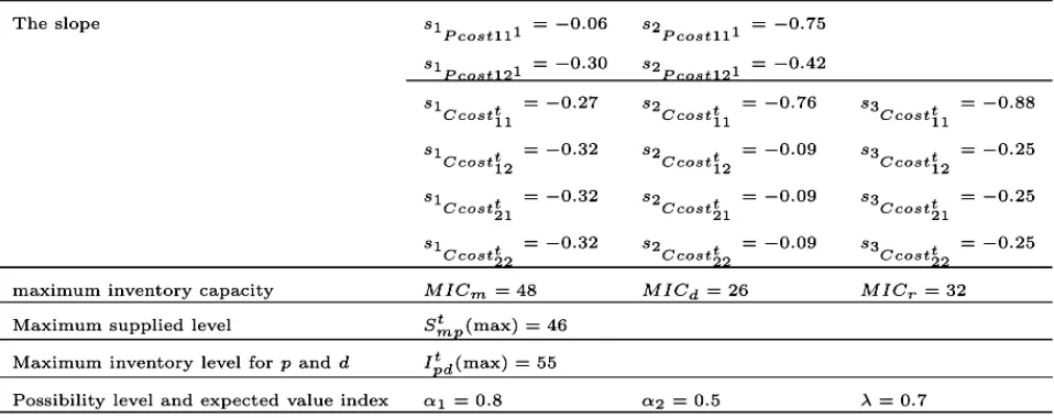
All the detailed data of supply chain system are gained from practical investigation. The bi-fuzzy variables are obtained based on previous data and experts' experience. In this case,

product cost per unit and stock carrying cost are considered as multiple breakpoint function as shown in Figure 2. The detailed information is shown in Table 1 ~ 5.

Table 1. Product cost per unit (multiple breakpoint function as shown in Figure 2)

Table 2. Transportation cost from manufacturer to distribution center

Table 3. Transportation cost from distribution center to retailer

Table 4. Stock carrying cost (multiple breakpoint function as shown in Figure 2)

5.1. The results

The parameters of MO-APSO for the multiple objective SCM problem are: swarm size popsize L = 50, iteration max T = 100, personal and global best position acceleration constant cp = cg = 2, inertia weight w(1) = 0.4, w(T) = 0.9. After dealing with the bi-fuzzy variables by the hybrid crisp approach in section 3, we use Matlab 7.0 and Visual C++ language on an Inter Core I7 M370, 2.40 GHz, with 2048 MB memory, and take the data into the computer program, the optimal solution of SCM model is generated by MO-APSO (see Figure 8).

Figure 8. The Pareto optimal solutions

Following Figure 8, DMs could choose the satisfactory scenarios from these pareto-optimal solutions according to the actual situation. For example, if DMs determine that the objective of total cost is the more important factor, they may allow a decreased average safe inventory levels. Thus, they would choose the far left pareto-optimal solutions.

5.2. Sensitivity analysis

In order to evaluate the effect of variations in model parameters, sensitivity analysis is

performed. For illuminating the sensitivity clearly, we changed the value of

α

2,

α

1, and λ in

turn, then compared the corresponding results to analyze the effect of each parameter. This work can provide the necessary information to the DMs for choosing the value of each parameter when considering the actual situation.

First, let

α

1 still be 0.8 as before, and

α

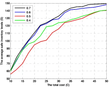
2 = 0.4, 0.3, 0.2, respectively. Then, we get Figure 9.

Finally, let

α

1 still be 0.8 and

α

2 still be 0.5, λ = 0.6, 0.5, 0.4, respectively. Then we gain 11.

Based on the sensitivity analysis of the results, the bi-fuzzy nonlinear MODM model for SCM is proved to be sensitive to the possibility level

α

1.

Figure 9. The sensitivity of α2 Figure 10. The sensitivity of α1

Figure 11. The sensitivity of λ

In practice, the DMs can change the parameters

α

1,

α

2 and λ to obtain the different solutions

under the different levels of parameters. The solutions reflect different optimistic-pessimistic attitudes for uncertainty and different predictions of possibility levels.

6. Conclusions and further research

Considering the complex fuzzy environment, a nonlinear MODM model for SCM with quantity discount policy is presented in this paper. The bi-fuzzy variables are transformed into the trapezoidal fuzzy variables by the DMs's degree of optimism

α

1 and

α

2, which are de-fuzzified

effectiveness, the proposed model and algorithm are applied to a typical example of SCM problem.

The main contributions of this study are as follows: (1) The bi-fuzzy variable is employed in the nonlinear MODM model of SCM to characterize the hybrid uncertain environment, and this work is original. (2) The proposed model is transferred to an equivalent crisp on by the DMs's degree of optimism and the expected value index. For solving the complex model, MO-APSO is designed as the solution method. (3) The study focuses on the SCM under complex fuzzy environment in SCM, which has a great practical significance.

The area for future research has two aspects: firstly, more realistic factors and constraints for SCM with complex hierarchical organization structure should be considered; secondly, more efficient heuristic methods should be designed to solve this nonlinear MODM model. Both areas are important and worth the concern.

Acknowledgment

This research was sponsored by Jiangsu Provincial Natural Science Foundation of China (Grant No. BK20130753), Fundamental Research Funds for the Central Universities (Grant No. JGQN1403, No. 30920130132012), “985” Program of Sichuan University “Innovative Research Base for Economic Development and Management”. We would like to give our great appreciates to all editors who contributed this research.

References

Al-e-hashem, S., Malekly, H., & Aryanezhad, M. (2011). A multi-objective robust optimization model for multi-product multi-site aggregate production planning in a supply chain under uncertainty. International Journal of Production Economics, 134, 28-42.

http://dx.doi.org/10.1016/j.ijpe.2011.01.027

Altiparmak, F., Gen, M., Lin, L., & Paksoy, T. (2006). A genetic algorithm approach for multi-objective optimization of supply chain networks. Computers & Industrial Engineering, 51(1), 196-215. http://dx.doi.org/10.1016/j.cie.2006.07.011

Arikan, F. (2013). A fuzzy solution approach for multi objective supplier selection. Expert Systems with Applications, 40(3), 947-952. http://dx.doi.org/10.1016/j.eswa.2012.05.051

Coello, C., & Lechuga, M. (2002). MOPSO: A proposal for multiple objective particle swarm optimization. In Proceedings of the 2002 Congress on Evolutionary Computation, 1051-1056.

Dubois, D., & Prade, H. (1988). Possibility Theory: An Approach to Computerized Processing of Uncertainty. New York: Plenum. http://dx.doi.org/10.1007/978-1-4684-5287-7

Garg, H., & Sharma, S. (2013). Multi-objective reliability-redundancy allocation problem using particle swarm optimization. Computers & Industrial Engineering, 64(1), 247-255.

http://dx.doi.org/10.1016/j.cie.2012.09.015

Giannoccaro, I., Pontrandolfo, P., & Scozzi, B. (2003). A fuzzy echelon approach for inventory management in supply chains. European Journal of Operational Research, 149(1), 185-196.

http://dx.doi.org/10.1016/S0377-2217(02)00441-1

Kennedy, J., & Eberhart, R. (1995). Particle swarm optimization. In Proceedings of the IEEE Conference on Neural Networks, 1942-1948. Piscataway: IEEE Service Center.

Kennedy, J., & Eberhart, R. (2001). Swarm Intelligence. Morgan Kaufmann.

Knowles, J., & Corne, D. (2000). Approximating the nondominated front using the pareto archived evolution strategy. Evolution Computation, 8, 149-172.

http://dx.doi.org/10.1023/A:1013771608623

Liu, B. (2002). Toward fuzzy optimization without mathematical ambiguity. Fuzzy Optimization and Decision Making, 1(1), 43-63. http://dx.doi.org/10.1023/A:1013771608623

Liu, Y., & Xu, J. (2006). A class of bifuzzy model and its application to single-period inventory problem. World Journal of Modelling and Simulation, 2(2), 109-118.

Luhandjula, M. (1987). Multiple objective programming problems with possibility coefficients. Fuzzy Sets and Systems, 21, 135-145. http://dx.doi.org/10.1016/0165-0114(87)90159-X

Nahmias, S. (1978). Fuzzy variables, Fuzzy Sets and Systems, 1, 97-110.

http://dx.doi.org/10.1016/0165-0114(78)90011-8

Shi, Y., & Eberhart, R. (1998). Particle swarm optimization. In Proc. IEEE Int. Conf. on Neural Networks, 69-73.

Simchi-Levi, D., Kaminsky, P., & Simchi-Levi, E. (2000). Designing and Managing the Supply Chain. New York: Irwin McGraw-Hill.

Tavakkoli-Moghaddam, R., Azarkish, M., & Sadeghnejad-Barkousaraie A. (2011). A new hybrid multi-objective Pareto archive PSO algorithm for a bi-objective job shop scheduling problem. Expert Systems with Applications, 38(9), 10812-10821. http://dx.doi.org/10.1016/j.eswa.2011.02.050

Torabi, S., & Hassini, E. (2008). An interactive possibilistic programming approach for multiple objective supply chain master planning. Fuzzy Sets and Systems, 159(2), 193-214.

http://dx.doi.org/10.1016/j.fss.2007.08.010

Wang, J., & Shu, Y. (2008). Fuzzy decision modeling for supply chain management. Fuzzy Sets and Systems, 150(1), 107-127. http://dx.doi.org/10.1016/j.fss.2004.07.005

Wei, C., Liang, G., & Wang, M. (2007). A comprehensive supply chain management project selection framework under fuzzy environment. International Journal of Project Management, 25(6), 627-636. http://dx.doi.org/10.1016/j.ijproman.2007.01.010

Xu, J., & Liu, Y. (2008). Multi-objective decision making model under fuzzy random environment and its application to inventory problems. Information Sciences, 178, 2899-2914. http://dx.doi.org/10.1016/j.ins.2008.03.003

Xu, J., & Yan, F. (2011). A multi-objective decision making model for the vendor selection problem in a bifuzzy environment. Expert Systems with Applications, 38(8), 9684-9695.

http://dx.doi.org/10.1016/j.eswa.2011.01.168

Xu, J., & Zhou, X. (2011). Fuzzy-Like Multiple Objective Decision Making. Berlin Heidelberg: Springer-Verlag.

Yan, L. (2009). Risk Curve and Bifuzzy Portfolio Selection. Journal of Mathematics Research, 1(2), 193-198. http://dx.doi.org/10.5539/jmr.v1n2p193

Zadeh. L. (1965). Fuzzy sets. Information and Control, 8, 338-353.

http://dx.doi.org/10.1016/S0019-9958(65)90241-X

Zadeh. L. (1978). Fuzzy sets as a basis for a theory of possibility. Fuzzy Sets and Systems, 1, 3-28. http://dx.doi.org/10.1016/0165-0114(78)90029-5

Zhang, G., Shao, X., Li, P., & Gao, L. (2009). An effective hybrid particle swarm optimization algorithm for multi-objective flexible job-shop scheduling problem. Computers & Industrial Engineering, 56(4), 1309-1318. http://dx.doi.org/10.1016/j.cie.2008.07.021

Journal of Industrial Engineering and Management, 2014 (www.jiem.org)

Article's contents are provided on a Attribution-Non Commercial 3.0 Creative commons license. Readers are allowed to copy, distribute and communicate article's contents, provided the author's and Journal of Industrial Engineering and Management's names are included.