Networks in Conflict: Theory and Evidence from the Great War of
Africa
∗Michael D. K¨onig†, Dominic Rohner‡, Mathias Thoenig§, Fabrizio Zilibotti¶
January 6, 2015
Abstract
We study from both a theoretical and an empirical perspective how a network of military alliances and enmities affects the intensity of a conflict. The model combines elements from network theory and from the politico-economic theory of conflict. We postulate a Tullock contest success function augmented by an externality: each group’s strength is increased by the fighting effort of its allies, and weakened by the fighting effort of its rivals. We obtain a closed form characterization of the Nash equilibrium of the fighting game, and of how the network structure affects individual and total fighting efforts. We then perform an empirical analysis using data on the Second Congo War, a conflict that involves many groups in a complex network of informal alliances and rivalries. We estimate the fighting externalities, and use these to infer the extent to which the conflict intensity can be reduced through (i) removing individual groups involved in the conflict; (ii) pacification policies aimed at alleviating animosity among groups.
∗We would like to thank Andr´e Python, Sebastian Ottinger and Nathan Zorzi for excellent research assistance. We are grateful for helpful comments from Daron Acemoglu, Alberto Alesina, Ernesto Dal Bo, Alessandra Casella, Melissa Dell, David Hemous, Macartan Humphreys, Massimo Morelli, Benjamin Olken, Maria Saez Marti, Uwe Sunde, Fernando Vega-Redondo, David Yanagizawa-Drott, Giulio Zanella, and conference and seminar participants of the ESEM-Asian Meeting (Taipei, 2014), IEA World Congress (Jordan, 2014), NBER SI 2014, and at the uni-versities of Bocconi, Bologna, CERGE-EI, Columbia, Harvard, MIT, European University Institute, IMT, INSEAD, IRES, Lausanne, LSE, Luxembourg, Marseille-Aix, Munich, Nottingham, Pompeu Fabra, SAET, Southampton, St. Gallen, Toulouse, ULB and Zurich. Mathias Thoenig acknowledges financial support from the ERC Starting Grant GRIEVANCES-313327.
†Department of Economics, University of Zurich. Email: [email protected].
‡Department of Economics, University of Lausanne. Email: [email protected]. Dominic Rohner gratefully acknowledges funding from the Swiss National Fund grant 100017 150159 on ”Ethnic Conflict”.
1
Introduction
Alliances and enmities among armed actors – be they rooted in history or in mere tactical consid-erations – are part and parcel of warfare.1 In many episodes, especially in civil conflicts, they are shallow links that are not sanctioned by formal treaties or war declarations. Even allied groups retain separate agendas and pursue self-interested goals in competition with each other. The com-mand of armed forces remains decentralized, and coordination is minimal.
Understanding the role of informal networks is important, not only for predicting outcomes, but also for implementing policies to contain or put an end to violence. These may be diplomatic initiatives promoted by international organizations to restore dialogue and reduce animosity be-tween conflict participants, or military interventions of external forces against specific groups. Yet, with only few exceptions, the existing political and economic theories restrict attention to conflicts among a small number of players, and do not consider network aspects. In this paper we construct a theory of conflict focusing explicitly on informal networks of alliances and enmities, and apply it econometrically to the study of the Second Congo War (1998-2003) and its aftermath.
The theoretical benchmark is a contest success function, henceforth CSF (see, e.g., Grossman and Kim 1995, Hirshleifer 1989, Skaperdas 1992). In a standard CSF, the share of the prize accruing to each group is determined by the amount of resources (fighting effort) that each of them commits to the conflict. In our model, the network of alliances and enmities modifies the sharing rule of a standard CSF by introducing additional externalities. More precisely, we assume that the share of the prize accruing to group i is determined by the group’s relative strength, which we label
operational performance, henceforth OP. In turn, the OP is determined by group i’s own fighting effort and by the fighting effort of its allied and enemy groups. The fighting effort of group i’s allies increases group i’s OP, whereas the fighting effort of its enemies decreases it. Thus, each group’s fighting effort affects positively its allies’ OP and negatively its enemies’. Instead, the costs of fighting are borne individually by each group. This raises a motive for strategic behavior among both enemy and allied groups. In particular, there is not even coordination between allies: all agents determine their effort in a non-cooperative way, and alliances are loose links.2 The complex externality web affects the optimal fighting effort of all groups.
We provide an analytical solution for the Nash equilibrium of the game. Absent other sources of heterogeneity, the fighting effort of each agent hinges on a measure of network centrality which is related to the Bonacich centrality (Ballester, Calvo-Armengol and Zenou 2006). Our centrality is approximately equal to the sum of the Bonacich centrality related to the network of enmities, and the (negative-parameter) Bonacich centrality related to the network of alliances. The equilibrium share of the prize accruing to each player and the associated welfare (i.e., the share of the prize net of the fighting effort) have simple expressions. Intuitively, a group’s welfare is increasing in the number of its allies and decreasing in the number of its enemies.
The ultimate goal of the theoretical analysis is to predict how the network of military alliances and rivalries affects the overall conflict intensity. This is measured by the sum of the fighting efforts
1Ghez (2011) distinguishes between tactical, historical and natural alliances. Tactical alliances are formed ”to
counter an immediate threat or adversary that has the potential to challenge a state’s most vital interests” (p. 20). They are instrumental and often opportunistic in nature. Historical alliances are more resilient insofar as they hinge on a historical tradition of cooperation. However, they often remain informal. Natural alliances imply a more profound shared political culture and vision of the world (e.g., Western Europe and the U.S.). Contrary to tactical and historical alliances, natural alliances often are formalized relationships. Our study focuses on tactical and historical alliances/enmities. In our theory, natural allies can be viewed as merged actors acting in a perfectly coordinated fashion.
2In some historical examples alliances are more than shallow links. Our theory can incorporate strong alliances
of all contenders (total rent dissipation), which is our measure of the welfare loss associated with a conflict. We show that network externalities are a key driver of the escalation or containment of violence.
As an illustrative example, we analyze a ”regular” network, in which the number of alliances and enmities is invariant across groups. We show that conflict intensity and rent dissipation are maximized when all groups are connected by enmity links. In this case, the outcome is a Hobbesian pre-contractual homo homini lupus society. When externalities are sufficiently strong, the cost of conflict may offset the social surplus in this society. To the opposite extreme, conflict and rent dissipation are minimized (and, possibly, vanish) in networks where all groups are allied, as in Rousseau’s well-ordered society governed by the social contract. The well-ordered society may be a surprising outcome in a non-cooperative contest between self-interested agents. The crux of the result is that the marginal product of fighting effort decreases in the number of alliances, because they dilute the marginal benefit from exercising individual fighting effort. For sufficiently strong alliance externalities, the incentive to fight vanishes altogether. The standard free-riding problem has a benign effect in our model, since war effort has no social value. The peaceful outcome can be viewed as representing a society in which the system of institutional checks and balances reduces the return to opportunistic behavior.
In the second part of the paper, we perform an empirical analysis based on the structural equa-tions of the model. We focus on the Second Congo War, sometimes referred to as the ”Great African War”. This is a big conflict, with an estimated death toll of 3-to-5 million lives (Autesserre 2008; Olsson and Fors 2004). It involves many groups, and a rich network of alliances and enmities.3 To identify the network of alliances and enmities we use information from the Stockholm International Peace Research Institute (SIPRI), supplemented by information from the Armed Conflict Loca-tion Event Database (ACLED). We assume that the network is exogenous and time-invariant – an assumption that conforms with the data for the period considered (see the discussion in section
3.3) – and proxy fighting effort by the number of fighting events in which each group is involved. The estimated networks of enmities and alliances feature numerous intransitivities, showing that the Second Congo War can by no means be described as a fight between two unitary opposing camps (see Figure6below). Our estimation strategy exploits panel variations in the yearly fighting efforts exerted by 85 armed groups over the 1998-2010 period. Controlling for group fixed effects and time-varying unobserved heterogeneity we regress the individual fighting effort of each group on the total fighting efforts of its degree-one allies and enemies, respectively. Since these are en-dogenous and subject to a reflection problem which is standard in regressions involving networks (see Bramoull´e, Djebbari and Fortin 2009; Liuet al. 2011), we use an IV strategy similar to that used by Acemoglu, Garcia-Jimeno and Robinson (2014). In particular, our identification exploits the exogenous variation in the average weather conditions facing, respectively, the set of allies and of enemies of each group. Our focus on weather shocks is motivated by the recent literature documenting that these have important effects on fighting intensity (see Dell 2012, Hidalgo et al.
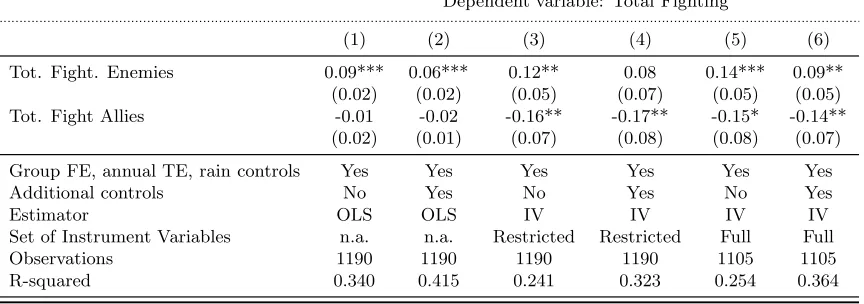
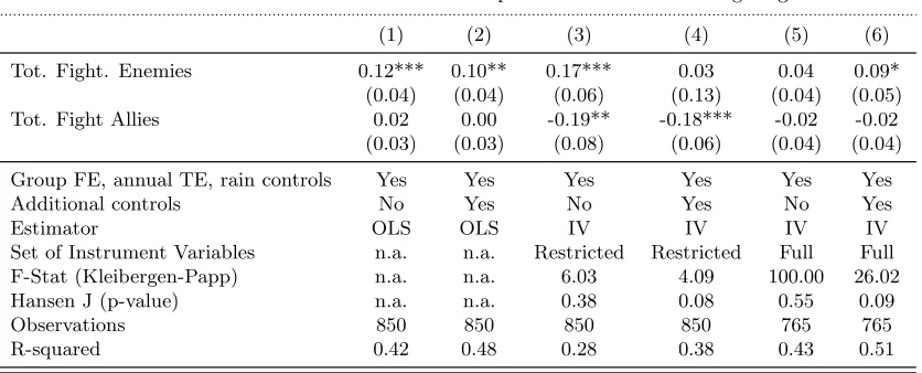
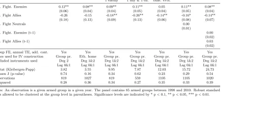
2010, Jia 2014, Miguel, Satyanath and Sergenti 2004, and Vanden Eynde 2011). Without imposing any restriction on the estimation procedure, we find that the two estimated externalities have the (opposite) sign pattern, which aligns with the predictions of the theory.
After estimating the size of the network externalities, we perform two sets of policy-oriented counterfactual experiments. First, we remove sequentially each of the groups in conflict while letting all surviving group re-optimize their fighting effort. This key-player analysis is a policy-relevant exercise, as it can help international authorities to single out armed groups whose decommissioning would be most effective for scaling down a conflict. Interestingly, we find that while on average
3More details about the historical context of this conflict are provided in Section3.1.
more active groups have a higher rank in the key player analysis, the relationship is far from one-to-one. For instance, the two factions of the Rally for Congolese Democracy (RCD) – Goma and Kisangani factions – rank, respectively, first and third in terms of their involvement in war episodes. Yet, their hypothetical removal would not contribute much to scaling down the conflict, because of their position in the network. According to our estimates, removing RCD-K would actually increase total violence, as the muted fighting of this group would be more than offset by the average increase in the effort of other armed groups. In contrast, the removal of the Hutu rebel group denominated Democratic Forces for the Liberation of Rwanda (FDLR) would yield a 14% reduction in violence. Our analysis also highlights the prominent role of foreign actors: eight out of the twenty groups bearing the largest responsibility for the escalation of violence are foreign national armies. Removing all foreign troops would reduce total violence by 24%, a large effect.
We also study a policy aimed at pacifying armed groups without removal, i.e., rewiring enmity links into neutral or alliance relationships. First, we show that pacifying all enmities in the Demo-cratic Republic of Congo (henceforth, DRC) would yield a reduction in fighting by between 54% and 91%. Next, we show that a more realistic policy aiming to pacify individual groups could also be effective. For instance, rewiring all enmities of the FDLR into neutral relationships would yield a de-escalation of the conflict by 13%.
Our contribution is related to various strands of the existing literature. First, our paper is linked to the growing literature on the economics of networks (e.g., Acemoglu and Ozdaglar 2011, Bramoull´e, Kranton, and d’Amours 2014, Jackson 2008, Jackson and Zenou 2014). There exist only very few papers in the literature studying strategic interactions of multiple agents in networks of conflict. Franke and ¨Ozt¨urk (2009) study agents being embedded in a network of bilateral conflicts, where agents can choose their fighting efforts to attack their neighbors. However, they do not allow for alliances. Moreover, they only characterize equilibrium efforts for particular networks (regular, star-shaped, and complete bipartite graphs), while we provide an equilibrium characterization for any network structure. Huremovic (2014) extends their model introducing endogenous fighting efforts in contests. His model differs from ours in several respects: there are no alliances, and the conflict is restricted to a collection of pairwise contests (while in our model many agents compete over a common prize). Neither of these studies tests the model empirically.
Two recent theoretical papers study the endogenous formation of networks in models of conflict. Hiller (2012) considers a model where agents can form alliances to coerce payoffs from enemies with fewer friends. Jackson and Nei (2014) study the formation of alliances in multilateral interstate wars and the implications on trade relationships between them, showing that trade can have a mitigating effect on conflicts. Neither of these papers consider, as we do, an endogenous choice of fighting effort. Different from these papers, we do not analyze the determinants of the network, which we infer from the data and treat as exogenous. Extending the analysis of endogenous network formation to large-scale networks including both enmities and alliances like the one in the Congo War is a challenging endeavor that is beyond the scope of this research.4
All of the above papers provide theoretical contributions. Our paper provides an estimation of the model based on the structural equations of the theory, and uses the estimates of the structural parameters to perform a key player analysis. In this sense, our paper is related to recent work by Acemoglu, Garcia-Jimeno and Robinson (2014) who estimate a political economy model of public
4From an empirical standpoint, most group characteristics that determine whether each two groups are friends,
goods provision using a network of Colombian municipalities. Their empirical strategy is related to ours, although they use historical variations in players’ characteristics while we use panel variations (exogenous shocks in rainfall).
The key player analysis in strategic games with networks is pioneered by Ballester, Calvo-Armengol and Zenou (2006). The authors determine equilibrium effort choices in a game of strategic complements between neighboring nodes, and identify key players, i.e. the agents whose removal reduces equilibrium aggregate effort the most. However, their payoff structure is substantially different from ours, and does not incorporate an environment in which agents compete for common resources. More recently, the key player policy has been studied empirically. Liuet al. (2011) test the key player policy for juvenile crime in the United States, while Lindquist and Zenou (2013) identify key players for co-offending networks in Sweden.
Further, our study is broadly related to the growing politico-economic conflict literature. Pa-pers in this literature typically focus on settings with two large groups facing each other, without considering network relationships. A few papers consider multiple groups comprising each a large number of players, and study collective action problems. Esteban and Ray (2001) show that the Olson paradox does not generally hold and that sometimes large groups can be more effective than small groups. To this purpose they build a model with n different groups composed each of a varying number of individual players. Their model is different and complementary to ours: they have no network structure, but focus on a setting comprising ndifferent cliques, where there are no links between cliques. Related to that, Rohner (2011) constructs a conflict model allowing for naggregate ethnic groups comprising a given number of individual players.
Our paper also shares some commonalities with the literature on the role of alliances in settings with either three players, or with identical players (see the surveys in Bloch 2012, and Konrad 2009 and 2011). Some papers note that alliances may be socially desirable since they reduce rent dissipation in wars (e.g. Olson and Zeckhauser 1966). Other papers regard the mere existence of alliances as a ”puzzle” given the free-riding (collective action) problem they generate, and the fact that victorious coalitions must share resources when victorious (see Esteban and Sakovics 2004, Konrad and Kovenock 2009, and Nitzan 1991).
Finally, our paper is related to the empirical literature on civil war, and in particular to the recent literature that studies conflict using very disaggregated micro-data on geo-localised fighting events, such as for example Dube and Vargas (2013), Cassar, Grosjean, and Whitt (2013), La Ferrara and Harari (2012), Michalopoulos and Papaioannou (2013), Rohner, Thoenig, and Zilibotti (2013b). In a recent interesting paper on the conflict in the DRC, Sanchez de la Sierra (2014) studies how price shocks of particular metals (cobalt, gold) affect the incentives of armed groups to establish control of resource-producing villages in Eastern Congo.
The paper is organized as follows: Section2presents the theoretical model and characterizes the equilibrium; Section 3 discusses the application to the Second Congo War and presents the main estimation results. Section 4 performs a number of robustness checks, while Section 5 performs some policy counterfactual analyses (key player and pacification policies). Section 6concludes. An appendix contains some technical material.
2
Theory
2.1 Environment
We consider a population of n ∈ N agents (armed groups) whose interactions are captured by a
network G∈ Gn, where Gn denotes the class of graphs on n nodes (vertices). Each pair of agents can be in one of three states: alliance, enmity, or neutrality. We represent the set of bilateral states
by the matrix A = (aij)1≤i,j≤n where aij ∈ {−1,0,1}. More formally, A is the signed adjacency matrix associated with the network G, where, for alli6=j,
aij =
1, if iand j are allies,
−1, if iand j are enemies,
0, if iand j are in a neutral relationship.
Note that a neutral relationship is modeled as the absence of links.
Let a+ij ≡max{aij,0} and a−ij ≡ −min{aij,0} denote the positive and negative parts of aij, respectively. Then, aij = a+ij −a−ij, respectively, for all 1 ≤ i, j ≤ n. Similarly, A = A+−A− where A+ = (a+ij)1≤i,j≤n and A− = (a−ij)1≤i,j≤n. We denote the corresponding subgraphs as G+
andG−, respectively, so thatGcan be written as the graph joinG=G+⊕G−. Finally, we define by d+i ≡Pnj=1a+ij andd−i ≡Pnj=1a−ij,respectively, the number of allies and enemies of agenti.
The n agents compete for a prize whose total value is denoted byV > 0. We assume agents’ payoffs to be determined by a generalized Tullockcontest success function(CSF) (cf. Tullock 1980, and Skaperdas 1996). The CSF maps the relative fighting intensity each agent devotes to a conflict into the share of the prize he appropriates after the conflict. More formally, we postulate a payoff functionπi :Gn×Rn→Rgiven by
πi(G,x) =ζi+V
ϕi(G,x)
Pn
j=1ϕj(G,x)
−xi (1)
where ζi ≥0 is an exogenous endowment, x ∈ S is a vector describing the fighting effort of each agent, andϕi ∈R is agent i’s operational performance (OP). The latter is assumed to depend on
agenti’s own fighting effort, as well as on his allies’ and enemies’ efforts. More formally, we assume that
ϕi(G,x)≡xi+β n
X
j=1
a+ijxj−γ n
X
j=1
a−ijxj, (2)
where β, γ ∈[0,1] are spillover parameters from allies’ and enemies’ fighting efforts, respectively. Note that the specification of equation (2) implies no heterogeneity across agents other than their position (i.e., the number of allies and enemies) in the network. We introduce other sources of heterogeneity (e.g., military power) in Section 2.6below.
Equation (2) postulates that each agent’s OP increases in the total effort exerted by its allies and decreases in the total effort exerted by its enemies. These externalities compound with those already embedded in standard CSFs, which equation (2) nests as a particular case whena+ij =a−ij = 0 for all
iand j. In this case,πi(G,x) =
xi/Pnj=1xj
V −xi, and each agent’s effort imposes a negative externality on the other agents in the contest only by increasing the denominator of the CSF.
Consider, for example, a network such that a+kk′ = 1 and β > 0, for one and only one pair of agents (k, k′) (while a−ij = 0 for all i, j = 1, . . . , n). Then, πk(G,x) = V (xk+βxk′)/(Pn
i=1xi +β(xk +xk′))−xk. In this case, an increase in the effort of k′ affects the payoff of k via two channels: (i) the standard negative externality working through the denominator; (ii) the positive externality working through the numerator. Thus, holding efforts constant, an alliance between two agents increases the share of V jointly accruing to them, at the expenses of the remaining groups. To the opposite, enmity links strengthen the negative externality of the standard CSF.
In the Nash equilibrium characterized in Section 2.2 below, however, all groups’ OP is positive.5 Note further that there is no ”participation decision”, namely, belligerent groups cannot decide to abstain from the conflict and live from their endowment. This has a natural interpretation: groups cannot flee from the country, and not making any fighting effort would expose them to other armed groups’ looting and ransacking activity. For technical reasons, we impose a lower bound to the choice set, i.e., x∈ S = [x1,∞)×[x2,∞)×...[xn,∞).
2.2 Equilibrium Fighting Effort
In this section, we characterize the Nash equilibrium of the contest. More formally, each agent chooses effort (xi) non-cooperatively so as to maximizeπi(G,[xi,x−i]), givenx−i. The equilibrium is a fixed point of the effort vector.
Using equations (1)-(2) yields the following system of first order conditions (FOC), for i = 1,2, . . . , n:
∂πi(G,x) ∂xi
= 0 ⇐⇒ϕi= 1 1 +βd+i −γd−i
1− 1
V n
X
j=1
ϕj
n
X
j=1
ϕj.
We assume that, for all i:
βd+i −γd−i >−1. (3) This condition is both necessary and sufficient for the second order condition to hold for all players at the equilibrium (see Proposition 1 and its proof in Appendix A). In the empirical analysis, we check that this condition holds for our estimates of β and γ.
Rearranging terms allows us to obtain a simple expression for the equilibrium OP level,
ϕ∗i (G) = Λβ,γ(G)1−Λβ,γ(G)Γβ,γi (G)×V, (4) and for the share of the prize accruing toiin equilibrium,
ϕ∗i(G)
Pn
j=1ϕ∗j(G)
= Γ β,γ i (G)
Pn
j=1Γβ,γj (G)
, (5)
where
Γβ,γi (G)≡ 1
1 +βd+i −γd−i , and Λ
β,γ(G)≡1− 1
Pn
i=1Γβ,γi (G)
. (6)
Γβ,γi (G) is a measure of the local hostility level capturing the externalities associated with agent i’s first-degree alliance and enmity links. Both Γβ,γi (G) and Λβ,γ(G) are decreasing with β, and increasing with γ (see Lemma 3 in Online AppendixB). Note also that equation (1) implies that the share of the prize accruing to agent iincreases in the number of her allies and decreases in the number of her enemies.
Next, we characterize the equilibrium fighting effort, and show how it depends on the structure of the network.
5Nor do we impose any non-negativity constraint onx
i,given the linearity of the pay-off function. The zero effort level is a matter of normalization. One could rewrite the model by replacing the effort level xiwith (¯x+xi). All results would be unchanged.
Proposition 1. Assume that β +γ < 1/max{λmax(G+), d−max}, where λmax(A±) denotes the largest eigenvalue associated with the matrix A±. Assume, in addition, that condition (3) holds true. LetΓβ,γi (G) and Λβ,γ(G) be defined as in equation (6), and let
cβ,γ(G)≡ In+βA+−γA−−1Γβ,γ(G) (7)
be a centrality vector, whose generic element cβ,γi (G) describes the centrality of agent i in the network G. Then, under an appropriate restriction of the strategy space, S = [x1,∞)×[x2,∞)×
...×[xn,∞)⊂Rn, wherexi >−∞ ∀i= 1,2, . . . , n, there exists a unique interior Nash equilibrium of then–player simultaneous move game with payoffs given by equation (1), agents’ OPs in equation (2), where the equilibrium effort levels are characterized by
x∗i(G) =VΛβ,γ(G)1−Λβ,γ(G)cβ,γi (G) (8)
for all i= 1, . . . , n, where x∗i (G)> xi. Moreover, the equilibrium OP levels are given by equation (4), and the equilibrium payoffs are given by
π∗i(G) =πi(x∗, G) =V(1−Λβ,γ(G))
Γβ,γi (G)−Λβ,γ(G)cβ,γi (G). (9) The inequality β+γ < 1/max{λmax(G+), d−max} is a sufficient condition for the matrix in (7)
to be invertible. Equation (9) follows from the set of FOCs. Condition (3) ensures that, for all i = 1, . . . , n, agent i’s payoff, conditional on x∗−i, is locally concave, implying that the FOCs pin down a local maximum for all players.6 Formally, this guarantees that the strategy profile satisfying (9) is alocal Nash equilibrium (Alos-Ferrer and Ania 2001).7 To ensure that this strategy profile is, in addition, a Nash equilibrium in the standard sense, we must impose a lower bound on the state space to ensure in turn that, conditional on x∗−i, x∗i (G) is a best reply over the entire admissible region, [xi,∞).8
The centrality measure, cβ,γi (G), plays a key role in Proposition 1. Note, in particular, that the relative fighting efforts of any two agents equals the ratio between the respective centrality in the network:
x∗i(G) x∗j(G) =
cβ,γi (G) cβ,γj (G).
2.3 The Case of Small Externalities
While cβ,γi (G) depends, in general, on the entire network structure, it is instructive to consider networks in which the spillover parameters β and γ are small. In this case, our centrality measure can be approximated by the the sum of (i) the Bonacich centrality related to the network of enmities, G−, (ii) the (negative-parameter) Bonacich centrality related to the network of alliances,G+, and (iii) the local hostility vector, Γβ,γ(G).9
6In the rest of this section, we assume that the two conditions under which the Proposition is proven are satisfied.
In the empirical analysis, we will check that the estimates ofβandγand the adjacency matrix ensure that the FOCs characterize an interior Nash equilibrium.
7Alocal Nash equilibriumis a strategy profile such that no player has an incentive to operate a “small” deviation.
A formal definition is provided in Definition2in AppendixA. The lower bound on the state space ensures that, at the equilibrium, no player has an incentive to operateany feasible deviation.
8In Remark1in Appendix A we show that it is possible to compute a common lower bound in Proposition1, x, on the effort levelsxi, such thatπi(x∗−i, xi, G)−πi(x∗, G)<0 holds for alli= 1, . . . , nif x∈[x,∞)nand that
x < x∗
i for alli= 1, . . . , n.
9See the Online AppendixDfor a more detailed discussion of the Bonacich centrality. A discussion of the Bonacich
Lemma 1. Assume that the conditions of Proposition 1 are satisfied. Then, as β →0 andγ →0,
the centrality measure defined in equation (7) can be written as
cβ,γ(G) =b·(γ, G−) +b·(−β, G+)−Γβ,γ(G) +O(βγ),
whereO(βγ)involves second and higher order terms, and the (µ-weighted) Bonacich centrality with
parameterα is defined as b·(α, G)≡bΓβ,γ(G)(α, G) = (In−αA)−1Γβ,γ(G) =P∞k=0αkAkΓβ,γ(G).
Lemma 1 states that the centrality cβ,γ(G) can be expressed as a linear combination of the weighted Bonacich centralities b·(γ, G−), b·(−β, G+) and the vector Γβ,γ(G). Each Bonacich centrality gauges the network multiplier effect attached to the system of enmities and alliances, respectively. In particular, b·(γ, G−) captures how a group i is influenced by all its (direct and indirect) enemies.10 In the case of of weak network externalities (i.e. whenβ →0 andγ →0), the Bonacich centrality can be itself approximated as follows:
b·,i γ, G− = Γβ,γi (G) +γ n
X
j=1
a−ijΓβ,γj (G) +γ2 n
X
j=1
a−ij n
X
k=1
a−jkΓβ,γk (G) +O γ3,
b·,i(−β, G+) = Γβ,γi (G) + (−β) n
X
j=1
a+ijΓβ,γj (G) + (−β)2 n
X
j=1
a+ij n
X
k=1
a+jkΓβ,γk (G) +O β3.
Thus, Lemma1suggests that, when higher order terms can be neglected, our centrality measure is increasing inγ and in the number of first order and second order enmities, whereas it is decreasing inβ and in the number of first order alliances. Second order alliances have instead a positive effect on the centrality measure.11
Moreover, we can also obtain a simple approximate expression for the equilibrium efforts and the payoffs in Proposition 1.12
Lemma 2. Asβ →0 andγ →0, the equilibrium effort and payoff of agenti in networkG can be written as
x∗i(G) =V Aβ,γ(G)−B βd+i −γd−i +O(βγ), π∗i(G) =V Cβ,γ(G) +D βd+i −γd−i +O(βγ),
where Aβ,γ(G), B, Cβ,γ(G) and D are positive constants with Aβ,γ(G) and Cβ,γ(G) being of the order of O(β) +O(γ).
10The Bonacich centrality measure related to the network of hostilities,b
·,i γ, G−, measures as the local hostility levels along all walks reaching i using only hostility connections, where walks of length k are weighted by the geometrically decaying hostility externalityγk(see also the Online AppendixD). Due to the approximation, we only consider links up to order two.
11The intuition for this property is as follows. Ifiis allied withjandjis allied withk, an increase in the fighting
effort ofk reduces the fighting effort ofjand this, in turn, increases the fighting effort ofi. Consider, instead, the case in whichiis an enemy ofj andj is an enemy ofk. Then, an increase in the fighting effort ofkincreases the fighting effort ofjand this, in turn, increases the fighting effort ofi.
12See the proof of Lemma2in AppendixAfor the explicit expressions for the constantsAβ,γ(G), B, Cβ,γ(G) and
D.
It is useful to note that, whenβ=γ= 0,then Λβ,γ(G) = 1−n1,andcβ,γi (G) = 1.Then, the equilibrium expressions in Proposition1simplify tox∗
i(G) =V(n−1)/n2 andπ∗i(G) =V /n2which are the standard solutions in the Tullock CSF.
Lemma 2 shows that, when network externalities are small, an agent’s fighting effort increases in the weighted difference between the number of enmities (weighted by γ) and alliances (weighted by β), i.e. the net local externalities d+i β−d−i γ. The opposite is true for the equilibrium payoff, which is increasing in d+i β−d−i γ. Thus,ceteris paribus, an increase in the spillover from alliances (enmities), parameterized by β (γ), and an increase in the number of allies (enemies) decreases (increases) agent i’s fighting effort and increases (reduces) its payoff. Intuitively, an agent with many enemies tends to fight harder and to appropriate a smaller share of the prize, whereas an agent with many friends tends to fight less and to appropriate a large size of the prize.
One must remember, however, that this simple result may fail to hold true if β and γ are not small and higher-degree links have sizeable effects. In the empirical analysis below, we find that higher order terms cannot be ignored to draw both positive and normative implications.
2.4 Rent Dissipation and Key Player
In this section, we discuss normative implications of the theory. Our welfare measure is (minus) the total rent dissipation. Since V is exogenous, the rent dissipation equals the total equilibrium fighting effort:
RDβ,γ(G)≡ 1
V n
X
i=1
x∗i(G) = Λβ,γ(G)(1−Λβ,γ(G)) n
X
i=1
cβ,γi (G).
Since Pni=1π∗i(G) = V 1−RDβ,γ(G), minimizing rent dissipation is equivalent to maximizing welfare.
Next, we define the key player to be the agent whose removal triggers the largest reduction in rent dissipation (cf. Ballester, Calvo-Armengol and Zenou 2006).
Definition 1. Let G\{i} be the network obtained from G by removing agent i, and assume that the conditions of Proposition 1 hold. Then the key player i∗ ∈ N ≡ {1, . . . , n} ∪ ∅ is defined by
i∗ = arg max i∈N
n
RDβ,γ(G)−RDβ,γ(G\{i})o. (10)
Note that the welfare difference RDβ,γ(G)−RDβ,γ(G\{i}) can be interpreted as the maximum cost that a benevolent policy maker is willing to pay to induce (or force) agentinot to participate in the contest. In Proposition 2 in the Online Appendix B, we show that the identity of the key player is related to the centrality measure defined in equation (7).13
2.5 Examples
In this section, we discuss two types of examples that illustrate general properties of the model. We consider, first, a regular graph where all agents have a symmetric position in the network. This graph is useful for showing how the number of alliances and enmities affects rent dissipation. Then, we consider a path graph with a core-periphery structure that highlights the importance of the centrality of agents in the network.
13The key player identified in equation (43) in Proposition2 in the Online AppendixBdiffers significantly from
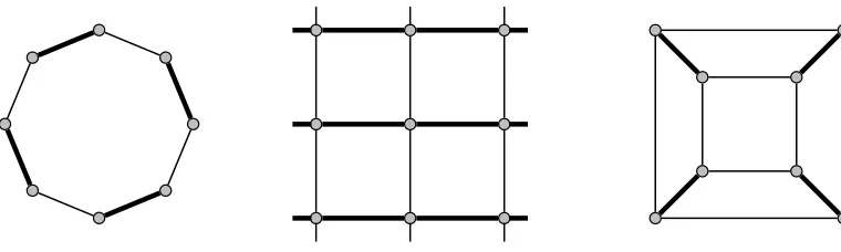
Figure 1: The figure shows three examples of regular graphsGk+,k−: The left panel shows a regular graph with k+ = k− = 1 (cycle), the middle panel shows a regular graph with k+ = k− = 2 (a lattice with periodic boundary conditions, i.e. a torus), and the right panel a Cayley graph with k+= 1 and k−= 2. Alliances are indicated with thick lines while enmities are indicated with thin lines.
2.5.1 Regular Graph
A regular network,Gk+,k−, has the property that every agentihasdi+=k+alliances andd−i =k− enmities. Regular graphs are tractable and enable us to perform comparative statics on the number of alliances or enmities in the network. Three examples of regular graphs are displayed in Figure
1.
Given the symmetric structure, there exists a symmetric Nash equilibrium such that all agents exercise the same effort. Moreover,ϕ∗i =ϕ∗ = 1/nfor alli= 1, . . . , n, implying an equal division of the pie. Under the conditions of Proposition1, the equilibrium effort and payoff vectors are given, respectively, by:
x∗ k+, k− ≡x∗i Gk+,k−=
1
1 +βk+−γk− − 1 n
×V
n, (11)
π∗ k+, k−≡π∗i Gk+,k−=
1 + (1 +n)(βk+−γk−) n(1 +βk+−γk−) ×
V
n. (12)
Standard differentiation implies that x∗ is decreasing in k+ and increasing in k−, whereas π∗ is increasing in k+ and decreasing ink−.Intuitively, alliances (enmities) reduce (increase) effort and rent dissipation by decreasing (increasing) the marginal return of individual fighting effort. This basic intuition gets confounded in general networks due to the asymmetries in higher-order links. However, the result is unambiguous in regular graphs.
The regular graph nests three interesting particular cases. First, if β = γ = 0, we have a standard Tullock game, with RD0,0 Gk+,k− = (n−1)/n. Second, consider a complete network of alliances (k+ = n−1), where, in addition, β → 1. Then, x∗ → 0 and RD1,γ(Gn−1,0) → 0,
i.e., there is no rent dissipation. Namely, the society attains peacefully the equal split of the surplus, as in Rousseau’s harmonious society. The lack of conflict does not stem here from social preferences or cooperation, but from the equilibrium outcome of a non-cooperative game between selfish individuals. The crux is the strong fighting externality across allied agents, which takes the marginal product of individual fighting effort down to zero. Third, consider, conversely, a society in which all relationships are hostile, i.e.,k− =n−1. Then, RDβ,γ(G0,n−1)→1 as γ →1/(n−1)2:
all rents are dissipated through fierce fighting and total destruction, as in Hobbes’ homo homini lupus pre-contractual society.
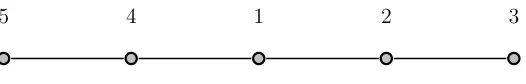
5 4 1 2 3
Figure 2: The figure shows a path graph,P5, with five agents.
0.00 0.01 0.02 0.03 0.04 0.05 0.06 0.07 0.16 0.17 0.18 0.19 0.20 x ∗ γ x∗ 1 x∗ 2 x∗ 3
0.00 0.01 0.02 0.03 0.04 0.05 0.06 0.07 0.010 0.015 0.020 0.025 0.030 0.035 0.040 π ∗ γ π∗ 1 π∗ 2 π∗ 3
0.0 0.1 0.2 0.3 0.4
0.00 0.05 0.10 0.15 x ∗ β x∗ 1 x∗ 2 x∗ 3
0.0 0.1 0.2 0.3 0.4
0.04 0.06 0.08 0.10 0.12 0.14 0.16 0.18 π ∗ β π∗1 π∗2
π∗3
Figure 3: The figure shows the equilibrium efforts (left panels) and payoffs (right panels) as functions ofγ andβfor two path graphs in which there are only enmity links (upper panels) and only alliance links (lower panels), respectively, forV = 1.
2.5.2 Path Graph
Next, we consider a path (core-periphery) graph,P5, with five agents, see Figure2. No link means
a neutral relationship. Suppose, first, that all links in Figure 2 are enmities. The upper left and upper right panel of Figure 3 show, respectively, effort levels and payoff for different values of γ. The ranking of the effort level yields x∗1(P5) > x∗2(P5) =x∗4(P5) > x∗3(P5) =x∗5(P5).14 Intuitively,
effort is proportional to the centrality in the network. The ranking of pay-offs is opposite: welfare increases as one moves from the center to the periphery. Fighting effort and payoffs are increasing and decreasing inγ, respectively.
Consider, next, the polar opposite case in which all links in Figure2 are alliances. The bottom left and right panels of Figure3show, respectively, effort levels and payoffs for different values ofβ.
14More formally, we have: x∗
1(P5) = V
2(γ(γ+2)−2)(γ(3γ2+γ−1)−1)
(5−7γ)2(3γ2−1) , x2(P5)
∗ =x∗
4(P5) = V
2((γ(3γ+5)−9)γ2+2)
(5−7γ)2(1−3γ2) and
x∗
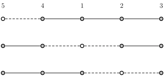
5 4 1 2 3
Figure 4: The figure shows three different graphs, P4, P2∪P2 and P3∪P1, obtained from a path
graph,P5, due to the removal of an agent.
The ranking of effort yields now, x∗2(P5) =x∗4(P5) < x∗1(P5)< x∗3(P5) =x∗5(P5).15 For a low range
ofβ’s, the peripheral agents, 3 and 5, exert the highest effort and earn the lowest payoff. However, for higher β’s, agents 3 and 5 earn a higher payoff than agent 1. Note that agents 2 and 4 exert the lowest effort, in spite of agent 1 being the most central player. The reason is that agents 2 and 4 are connected, respectively, to agents 3 and 5 who lie at the periphery of the network, and who have no other connections. Thus, agents 2 and 4 can free ride on the high effort exerted by 3 and 5.16 Finally, the efforts and payoffs of agents 1,3 and 5 are non-monotonic, due to the fact that, whenβ is high, there is more free riding. Agents 2 and 4 exert very low fighting effort, and induce substitution effects (i.e., higher effort) from their respective neighbors.
The results are consistent with Lemma 2. In the upper panel, asγ →0 the effort is lowest and payoff is highest for the agent who has the smallest number of enemies (i.e., agent 1).In the lower panel, asβ →0 the effort is highest for the agents who have only one ally (i.e., agents 3 and 5).
Finally, we perform a key player analysis. Figure4shows the three different graphs,P4,P2∪P2
andP3∪P1, obtained from removing one agent fromP5. When all links are enmities, the maximum
reduction in rent dissipation is attained by removing the central agent, 1. The reason is that, in this case, a graph with more walks (hence, stronger network feedback effects) amplifies fighting. Removing the central agent inP5(as displayed inP2∪P2) yields the largest reduction in the number
of walks, resulting in the lowest total fighting. In contrast, when all links are alliances, fighting is decreasing in the number of walks. In this case, the maximum reduction in rent dissipation is attained by removing a peripheral agent (either 3 or 5).
2.6 Heterogeneous Fighting Technologies
So far, we have maintained that all agents have access to the same technology turning fighting effort into OP. This was useful for keeping the focus sharply on the network structure. In reality, armed groups typically differ in size, wealth, access to weapons, etc. In this section, we generalize our model by allowing fighting technologies to differ across players. We restrict attention to additive heterogeneity, since this is crucial for achieving identification in the econometric model presented
15The analytical expressions arex∗
1(P5) =V
2(β2(β+1)(β(3β−10)+5)−2)
(7β+5)2(3β2−1) ,x ∗
2(P5) =V
2(β2(β(5−3β)+9)−2)
(7β+5)2(3β2−1) andx ∗
3(P5) =
V2((β−2)β−2)(β(β+1)(3β−1)−1) (7β+5)2(1−3β2) .
16This is related to the interpretation of the Bonacich centrality with a negative parameter. In this case a node
is more powerful to the degree that its connections themselves have few alternative connections (see Sec. 1.1.1 in Bonacich, 2007).
below.17
Suppose that agent i’s OP is given by:
ϕi(G,x) = ˜ϕi+xi+β n
X
j=1
a+ijxj−γ n
X
j=1
a−ijxj, (13)
where ˜ϕi is a group-specific shifter affecting OP (e.g., its military capability).18
In the appendix, we show that the equilibrium OP is unchanged, and continues to be given by equation (4). Likewise, equation (5) continues to characterize the share of the prize appro-priated by each agent. Somewhat surprising, the share of resources approappro-priated by group i, ϕ∗i(G)/Pnj=1ϕj∗(G), is independent of ˜ϕi. However, ˜ϕi affects the equilibrium effort exerted by groupiand its payoff. In particular, the vector of the equilibrium fighting efforts is now given by
x∗ = (In+βA+−γA−)−1(VΛβ,γ(G)(1−Λβ,γ(G))Γβ,γ(G)−ϕ˜), (14) where the definitions of Λβ,γ(G) and Γβ,γ(G) are unchanged (see Proposition 3 in the Online AppendixB).
Equation (13) will be the basis of our econometric analysis where we introduce both observable and unobservable sources of heterogeneity. In particular, time-varying shocks to ˜ϕ will be key for the econometric identification.
3
Empirical Application - The Second Congo War
In this section, we apply the theory to the recent civil conflict in the Democratic Republic of Congo (henceforth, DRC). Our goal is to estimate the externality parameters β and γ from the structural equation (13) characterizing the Nash equilibrium of the model. Equipped with point estimates of the structural parameters we test key restrictions imposed by the theory and perform counterfactual pacification policies. We start by presenting the historical context of the DRC conflict. Then, we discuss the data sources and how the network structure is observed from the data. Finally, we proceed to the econometric model and to the discussion of our identification and estimation procedure.
3.1 Historical Context
We study the Second Congo War, sometimes referred to as the ”Great African War”. Detailed accounts of this conflict can be found in Prunier (2011) and Stearns (2011). The DRC is the largest Sub-Saharan African country in terms of area, and is populated by about 75 million inhabitants. It is a classic example of a failed state. After gaining independence from Belgium in 1960, it expe-rienced recurrent political and military turbulence that turned it into one of the poorest countries in the world, despite its abundance of natural resources (including diamonds, copper, gold and cobalt). The DRC is also a very ethnically fragmented country with over 200 ethnic groups. The
17It is possible to solve for richer forms of heterogenity, such as a multiplicative one. However, we do not focus on
such alternative cases, since it becomes impossible to identify econometrically the parameters of the model.
18An alternative interpretation is to consider our model as the linear approximation of a logit-form CSF (cf.
Skaperdas, 1996). Consider the payoff function πi :Gn×Rn → R with πi(G,x) ≡ V eλϕi
(G,x)
Pn j=1eλϕj
(G,x) −xi, for all
i= 1, . . . , n, whereϕi(G,x) is the OP of agentigiven by equation (2). In the limitλ→0 we obtain the ratio form
πi(G,x) =V 1+λϕi(G,x)+O(λ
2)
n+λPn
j=1ϕj(G,x)+O(λ2)−xi=V
λ−1+ϕ
i(G,x)+O(λ)
nλ−1+Pn
Congo conflict is emblematic of the role of natural resource rents and of the involvement of many inter-connected domestic and foreign actors. In particular, the conflict involved three Congolese rebel movements, 14 foreign armed groups, and several militias (Autesserre 2008). In such complex and fragmented warfare, alliances and enmities play a major role.
The Congo Wars are intertwined with the ethnic conflicts in neighboring Rwanda and Uganda. The culminating event is the Rwandan genocide of 1994, where the Hutu-dominated government of Rwanda supported by ethnic militias such as the Interahamwe, persecuted and killed nearly a million of Tutsis and moderate Hutus in less than one hundred days. After losing power to the Tutsi rebels of the Rwandan Patriotic Front (RPF), over a million Hutus fled Rwanda and found refuge in the DRC, governed at that time by the dictator Mobutu Sese Seko. The refugee camps hosted, along with civilians, former militiamen responsible of the Rwandan genocide. These continued to clash with the Tutsi population living both in Rwanda and in the DRC, most notably in the Kivu region (Seybolt 2000).
As ethnic tensions escalated, a broad coalition centered around Uganda and Rwanda, but also comprising several other African states, supported the anti-Mobutu rebellion led by Laurent-D´esir´e Kabila’s Alliance of Democratic Forces for the Liberation of Congo (ADFL). The First Congo War (1996-97) ended with Kabila’s victory. However, the relationship of the new president of the DRC with his former Tutsi allies and his main foreign sponsors, Rwanda and Uganda, deteriorated rapidly. The Second Congo War erupted in 1998 where Kabila received the support of some former foreign allies (Angola, Chad, Namibia, Sudan and Zimbabwe) and of the Hutu militias that had previously supported Mobutu.19 His main enemies were Uganda, Rwanda and a network of rebel groups. Many rebel groups were linked to foreign powers: Uganda sponsored the Rally for Congolese Democracy - Kisangani (RCD-K), while the Congolese Liberation Movement (MLC), the Rally for Congolese Democracy - Goma (RCD-G) received support from Rwanda (Seybolt 2000). The heart of the war was the Eastern border and the conflict spread fast to the whole country, with many actors taking part in the conflict out of hostility to other specific actors. These include, among others, the anti-Ugandan rebel forces of the Allied Democratic Forces and the Lord’s Resistance Army, or the anti-Angolan UNITA forces.
The Second Congo War ended officially in 2003, although fighting is still going on today. It is the deadliest conflict since World War II, with between 3 and 5 million lives lost (Olsson and Fors, 2004; Autesserre, 2008). In spite of the numerous shifts that occurred in 1997, the web of alliances and enmities remained remarkably stable thereafter. As documented by Prunier (2011: 187ff), most alliances and enmities were determined by international and domestic factors of the countries involved, and remained constant over the entire conflict (at least until 2010, the extent of time covered by our data). Many groups chose their loyalties followingRealpolitik and trying to balance rising neighbors like South Africa or Sudan.
While many groups involved in the Second Congo War took stands vis-a-vis the DRC gov-ernment, there were flagrant violations of transitivity, and the conflict cannot be described as a coherent two-camp (pro- versus anti-DRC government) war. In Prunier’s words, ”the continent was fractured, not only for or against Kabila, but within each of the two camps” (2011: 187). Recurrent clashes erupted among the main factions - like in the case of the infamous violent clashes between RCD-G and RCD-K (Prunier 2011: 240ff; Turner 2007: 200). Even the historical alliance between Uganda and Rwanda, which was forged on ethnic and geopolitical grounds cracked a few times, resulting in important clashes between the two armies or between groups sponsored by ei-ther of them (Turner, 2007: 200). Similarly, ei-there was in-fighting among different pro-government paramilitary groups, such as the Mayi-Mayi militias, (cf. Prunier 2011: 281). The DRC army
19In 2001, Laurent-D´esir´e Kabila was assassinated, and was later replaced by his son Joseph Kabila.
itself was notoriously prone to internal clashes and mutinies, spurred by the fact that its units are segregated along ethnic lines and often correspond to former ethnic militias or paramilitaries that got integrated into the national army (cf. Prunier 2011: 305ff).20 In summary, far from being a war between two unitary alliances, the conflict engaged a complex web of alliances and enmities, with many non-transitive links.
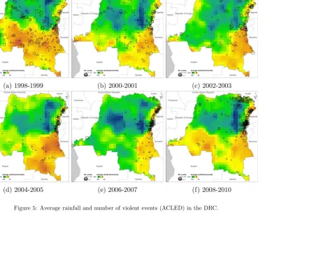
Two other aspects of the conflict are noteworthy. First, with the exception of the DRC armed forces, most actors were active in limited parts of the country. Ethnic militias (i.e., the vast majority of local armed groups) typically fought in territories adjacent to those where their affiliated population lived. Second, weather conditions were important in determining the intensity of the conflict in different regions. Figure5 displays the fighting intensity and average climate conditions for different ethnic homelands in the DRC.21 Weather conditions vary considerably both across regions of the DRC and over time.
3.2 Data
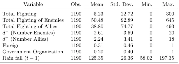
We build a panel dataset for the period 1998-2010 that includes both the official years of the Second Congo War (until 2003) and its turbulent aftermath. The unit of observation is at the fighting group×year level (annual frequency). The variables used in the estimations are built from a variety of data sources. We describe these and the construction of the variables in this section. The related summary statistics are displayed in Table 1.
Fighting –Our main data source is the Armed Conflict Location and Events Dataset (ACLED 2012).22 This dataset contains 4765 geo-localised violent events taking place in the DRC involving 85 fighting groups. For each such event, ACLED provides information on the exact location, the date and the identities of the involved groups – including information about which groups fight on the same side and which fight on opposite sides.23 In the recent literature ACLED has been used so far with the purpose of building geolocalized measurement of violence. Here, besides geolocalization, we also exploit bilateral information about which groups fight together or against each other to document the fine-grained structure of the network of alliances and enmities. To the best of our knowledge, our study is the first to exploit this information.
Our main dependent variable is group i’s yearly Fighting Effort. We measure xit as the sum over all ACLED fighting events involving groupiin year t. In the robustness section, we construct
20Turner (2007) describes a typical clash between army fractions in 2004: ”In the aftermath of the peace agreements
of Sun City and Pretoria, Congo was supposed to create a unified national army and civil-territorial administration. Some Rwandophone officers of North and South Kivu led the resistance tobrassage (intermingling) of officers and troops from various composants. The two most prominent of these were Colonel Jules Mutebutsi (a Munyamulenge from South Kivu) and General Laurent Nkunda (Rwandophone Tutsi allegedly from Rutshuru in Kivu). These officers led a mutiny against their superiors, and briefly took over the city of Bukavu (capital of South Kivu) (2007: 96).”
21The data used for generating this figure are discussed in detail below.
22This a well established data source in the literature. Recent papers using ACLED include, among others, Berman
et al. (2014), Cassar, Grosjean, and Whitt (2013), Michalopoulos and Papaioannou (2013), and Rohner, Thoenig, and Zilibotti (2013b).
23Here are three examples: On the 18th of May 1999 a battle took place between ”RCD: Rally for Congolese
Figure 5: Average rainfall and number of violent events (ACLED) in the DRC.
Table 1: Summary statistics.
Variable Obs. Mean Std. Dev. Min. Max.
Total Fighting 1190 5.23 22.72 0 300
Total Fighting of Enemies 1190 50.48 92.89 0 645 Total Fighting of Allies 1190 38.80 74.77 0 493
d−(Number Enemies) 1190 2.61 3.59 0 20
d+(Number Allies) 1190 2.24 3.41 0 18
Foreign 1190 0.31 0.46 0 1
Government Organization 1190 0.20 0.40 0 1
Rain fall (t−1) 1190 125.35 26.36 58.02 197.35
alternative measures of fighting effort by restricting the count to the more conspicuous events such as those classified by ACLED as battles or those involving fatalities.
Rainfall – For the purpose of our instrumentation strategy we build the yearly average of rainfall in the homeland of each fighting group. We use gauge-based rainfall measure from the Global Precipitation Climatology Centre (GPCC) (Schneideret al. 2011), at a spatial resolution of 0.5◦×0.5◦grid-cells. This dataset is widely used and is renowned for its precision and fine resolution. The homeland of a fighting group corresponds to the spatial zone of its fighting operations (i.e. convex hull containing all geolocalized ACLED events involving that group at any time during the period 1998-2010). Then, for each year t, we compute the average rainfall in the grid-cell of the homeland centroid. Alternative constructions are considered in our robustness analysis.24
One potential concern is that rain-gauges located at the ground level may be damaged by local fighting activities. Therefore, in the robustness section, we also use satellite-based rainfall measures. These are generally less precise, but it is safe to assume that the measurement error is uncorrelated with ground-level fighting. We use two alternative annual dataset. The first comes from the Global Precipitation Climatology Project (GPCP) from NOAA and has a spatial resolution of 2.5◦×2.5◦. The second is the Tropical Rainfall Measuring Mission (TRMM) from NASA at a resolution of 0.5◦×0.5◦. These dataset use atmospheric parameters (e.g. cloud coverage, light intensity) as indirect and noisy measures of rainfall. Hence both of these satellite-based measures are much less precise than the rain-gauge measure.
Covariates – The following variables are used to generate the set of control variables. Gov-ernment Organization is a binary variable equal to 1 for fighting groups that are officially affiliated to a domestic or foreign government. This amounts to 17 groups out of 85, corresponding to the military and police forces of Angola, Burundi, Chad, DRC, Namibia, Rwanda, South Africa, Sudan, Uganda, Zambia and Zimbabwe. The dummyForeign is equal to 1 for all foreign actors, and 0 for all fighting groups that originate from the DRC. In total 26 groups are coded as Foreign. Finally for all groups we compute the yearly amount of fighting events in which they are involved outside the DRC. The resulting variable,Fighting Effort Outside DRC, is used as proxy for the global scope of operation of a group.
24One option consists in averaging rainfall across all grid-cells of the homeland (not only at the centroid). As for
3.3 The Fighting Network
We estimate the network of alliances and enmities using two data sources. First, we use the Yearbook of the Stockholm International Peace Research Institute (SIPRI, see Seybolt, 2000). Second, we use the dyadic information provided by ACLED. Details are provided below.
As our primary criterion, we follow the classification provided by SIPRI, which lists alliances between the major actors, including both actors operating in the same region and groups fighting in different parts of the country but supporting each other logistically. The limitation of the SIPRI data is that they do not cover small armed groups and militias nor do they contain detailed information about bilateral enmity links.
For this reason, we also use the dyadic information provided by ACLED. In particular, we code two groups (i, j) as allies (i.e. a+ij = a+ji = 1) if they have been observed fighting on the same side in at least one occasion during the sample period, and if, in addition, they have never been observed fighting on opposite sides. Conversely, we code two groups asenemies (i.e. a−ij =a−ji= 1) if they have been observed fighting on opposite sides on at least two occasions, and they have never been observed fighting on the same side.25 We code all other dyads as neutral (i.e. a+
ij =a−ij = 0). Slightly less than 3% of the dyads are coded as allies, and slightly more than 3% are coded as enemies. The remaining dyads are classified as neutral, either because they were never involved jointly in any fighting event (93% of the dyads), or because of ambiguities, namely, the two groups were recorded fighting sometimes on the same side, and sometimes on opposite sides. The propor-tion of all dyads that are classified as neutral due to such an ambiguity is less than 1%. On average a group has 2.6 enemies and 2.2 allies (see Table 1).
Our methodology may raise three concerns. First, we assume a time-invariant network. One might fear that alliances and enmities get reshuffled throughout the war. From a historical per-spective it appears as if many changes in the system of alliances took place at the end of the First Congo War, but that alliances remain broadly stable thereafter (cf. Prunier 2011). However, one might worry that this broad pattern may not apply to small groups, whose behavior is not equally well-documented by the conflict literature. To get a sense of the potential importance of the problem, we search for instances in which there is a clear switch in the nature of a dyadic re-lationship in ACLED. A clear evidence of structural change would be that there exists a threshold yearT ∈(1998−2010) such that two groups would be classified as allies (enemies) if one restricted attention to the years up to T,while the same two groups would be classified as enemies (allies) if one considered the years after T.We have eight dyads, a mere 0.2% of the total 3570 dyads that conform with this pattern. This is a strong indication that in most of the 1% dyads for which an ambiguity arises, this ambiguity is due to occasional clashes between troops (or one-shot tac-tical alliances within a single battle) rather than to structural changes in system of alliances and enmities. This is reassuring for our assumption that the network is time-invariant.26
The second concern is that the construction of the network partly relies on the same ACLED data that we use to measure the outcome variable (i.e fighting). Here, let us emphasize two important differences. First, for the network we exploit the bilateral (dyadic) information which is not used to construct the outcome variable. Second, the network is time-invariant, whereas our econometric analysis exploits the time variations in fighting efforts, controlling for group fixed effects, as discussed in more detail below. To further alleviate this concern, in Section 4 we build
25Given that in our theoretical setting all groups are competing, by definition, for the same prize, we require at
least two instances of fighting against each other to code two groups asenemies. As shown below, our results are robust to alternative coding where groups areenemies when they fight against each other in at least one instance.
26To further alleviate this concern, in the robustness section we restrict the sample to 1998-2007, since there is
anedoctal evidence that after 2007 some militias were wiped out or absorbed by the DRC Army. The results are robust.
LRA
UNITA
FAA/M...
Uganda
Hutu
Burundi J. Kab.
SPLA/M Sudan FNL L. Kab. ADF RCD G... FDLR Rwand... Mayi-... CNDD-... Zimba... Chad Hutu RCD K. CNDP MLC DRC M... UPC Lendu ADFL RCD Namibia FNI Rwand... FPJC FRPI Hema Mutiny ALIR MRC NALU FLC South... DRC P... PARECO PUSIC Rwand... UPPS BDK Zambia RUD Enyele Lobala FRF APCLS Lendu
Un. M... F. DRC
Haut-... Mayi-... Mayi-... Minem... Bomboma Masunzu Wager... CNDD-... RCD N...
Figure 6: The figure shows the network of alliances and conflicts in the DRC. Thick lines indicate alliances, while thin lines indicate enmities. The nodes’ colors and sizes represent their centrality (cf. Section 2.2).
the network using SIPRI and ACLED data from the period 1998-2001, while the outcome variable uses the information for the period 2002-2010. This comes at a high cost in term of information loss since the conflict attains its highest intensity in the initial years. The results are robust, albeit less precisely estimated.
Third, we are likely to miss some network links. It is likely that we code as neutral some dyads that are in fact allies or enemies but did not participate into common fighting events (e.g. due to spatial distance). Such missing links create measurement errors that can bias the estimates of the fighting externalities (Chandrasekhar and Lewis, 2011). The strategy to tackle this issue is twofold. On the one hand, we check the robustness of our results to alternative coding rules of alliances and enmities.27 On the other hand, we perform Monte Carlo simulation to assess the bias associated with an imperfect observation of missing links.
Figure 6 illustrates the network of alliances and rivalries in DRC. Not surprisingly, the armed forces of DRC have the highest centrality. The other groups with a high centrality are the Rally for Congolese Democracy (Goma and Kisangani), the Mayi-Mayi militias, and the foreign armies of Rwanda, Uganda, Zimbabwe, Namibia, Sudan, and Angola. All these groups are known to have played a salient role in the Second Congo War.
27We consider a variety of alternative coding rules of alliances and enmities. In addition, we check the robustness
3.4 Econometric Model
The basis of our empirical analysis is Section 2.6, allowing for exogenous sources of heterogeneity in the OP of groups. Equation (13) can be turned into an econometric equation by assuming that the individual shocks ˜ϕi comprise both observable and unobservable shifters. More formally, we assume that ˜ϕi = z′iα+ǫi, where zi is a vector of group-specific observable characteristics, and ǫi is an unobserved shifter. Replacing xi and ϕi by their respective equilibrium values, yields the following structural equation:
x∗i =ϕ∗i (G)−β n
X
j=1
a+ijx∗j +γ n
X
j=1
a−ijx∗j −z′iα−ǫi. (15)
It is important to recall thatϕ∗i is fully characterized by the externality parameters and the time-invariant network structure, (β, γ, d−i , d+i ) , and is independent of the realizations of individual shocks (zi, ǫi) (see equation 4and Section 2.6). Our goal is to estimate the network parametersβ and γ. The estimation is subject to a simultaneity or reflection problem (Manski 1993; Boucher
et al. 2012), a common challenge in the estimation of network externalities. A related issue in this class of models is that it is difficult to separate contextual effects, i.e., the influence of players’ characteristics, from endogenous effects, i.e., the effect of outcome variables via network externalities. In our model, the endogenous effect is associated with the fighting effort exerted by a group’s allies and enemies. Although our theory postulates no contextual effect, it is plausible that omitted variables affectingx∗i are spatially correlated, implying that one cannot safely assume spatial independence ofǫi.Ignoring this problem might yield inconsistent estimates of the spillover parameters.
The reflection problem can be tackled by using instruments to obtain consistent estimates of the spillover effects. For instance, in a recent study on public good provision in a network of Colombian municipalities, Acemoglu, Garcia-Jimeno and Robinson (2014) use as instruments historical characteristics of local municipalities which are argued to be spatially uncorrelated. In our case, it is difficult to single out time-invariant group characteristics that affect the fighting efforts of a group’s allies or enemies without invalidating the exclusion restriction. For instance, cultural or ethnic characteristics of group iare likely to be shared by its allies. For this reason, we take the alternative route of identifying the model out of exogenous time-varying shifters affecting the fighting intensity of allies and enemies over time. This panel approach has the advantage that we can difference out any time-invariant heterogeneity, thereby eliminating the problem of correlated fixed effects.
Panel Specification – We maintain the assumption of an exogenous time-invariant network, and assume that the conflict repeats itself over several years. We abstract from reputational effects, and regard each period as a one-shot game. These are strong assumptions, but they are necessary to retain tractability. The variation over time in conflict intensity is driven by the realization of group-and time-specific shocks, amplified or offset by the endogenous response of the players which, in turn, hinges on the network structure. More formally, we allow bothx∗i and ˜ϕi to be time-varying:
˜
ϕit=z′itα+ei+ǫit. (16)
Here,zit is a vector of observable shocks with coefficients α,ei is a vector of (unobservable) time-invariant group-specific characteristics, and ǫit is a i.i.d., zero-mean unobservable shock. Rainfall measures are examples of observable shifters zit that will be key for identification. The panel analogue of equation (15) can then be written as:
Fightit=fei−β×Fightall
it +γ×Fight
ene
where
Fightit =x∗
it
Fightall
it = n
X
j=1
a+ijx∗jt,
Fightene
it = n
X
j=1
a−ijx∗jt,
fei =−ϕ∗
i (G)−ei. (18)
The panel dimension allows us to filter out any time-invariant correlated effects by including group fixed effects fei. However, due to the reflection problem discussed above, the two covariates Fightall
it (Total Fighting of Allies) andFight
ene
it (Total Fighting of Enemies) are correlated with the error terms. In other words, there is an endogeneity problem because the effort of group i’s allies and enemies are affected by group i’s effort. Thus, OLS estimates are inconsistent.
The problem can be addressed by an instrumental variable strategy. This requires identifying exogenous sources of variations in the fighting efforts of group i’s allies and enemies that do not influence groupi’s fighting effort directly. To this aim, we use time-varying climatic shocks (rainfall) impacting the homelands of armed groups. In line with the empirical literature and historical case studies (Dell 2012), we focus on local rainfall as a time-varying shifter of OP, and hence the fighting effort of allies and enemies. We expect groups affected by positive rainfall shocks to fight less, since local rainfall increases the agricultural surplus, thereby pushing up the reservation wages of productive labor and, hence, the opportunity cost of fighting. This channel linking rainfall to conflict has been documented, among others, by Jia (2014), Hidalgo et al. (2010), Miguel et al.
(2004), Vanden Eynde (2011).
To be a valid instrument, rainfall in the homelands of the allies (enemies) must be correlated with the allies’ (enemies’) fighting efforts. We show below that this is so in the data. The exclusion restriction requires that rainfall in the homelands of group i’s allies and enemies have no direct effect on fighting efforts of groupi. Although rainfall is likely to be spatially correlated, due to the proximity of the homelands of allied or enemy groups, this is not a problem since we control for the rainfall in group i’s homeland in the second-stage regression. For instance, suppose that group ihas a single enemy, groupk,and that the two groups live in adjacent homelands. Rainfall in k’s homeland is correlated with rainfall in i’s homeland. However, rainfall in k’s homeland is a valid instrument for k’s fighting effort, as long as rainfall ini’s homeland is included as a non-excluded instrument. A potential issue arises if rainfall is measured with error, and measurement error has a non-classical nature. We tackle this issue below in the robustness analysis.