ISSN 2324-805X E-ISSN 2324-8068 Published by Redfame Publishing URL: http://jets.redfame.com
What’s in a Coefficient? The “Not so Simple” Interpretation of
R
2, for
Relatively Small Sample Sizes
Nizar Zaarour1, Emanuel Melachrinoudis1 1
Northeastern University, USA
Correspondence: Nizar Zaarour, Northeastern University, USA.
Received: August 28, 2019 Accepted: September 19, 2019 Online Published: September 19, 2019
doi:10.11114/jets.v7i12.4492 URL: https://doi.org/10.11114/jets.v7i12.4492
Abstract
There are several misconceptions when interpreting the values of the coefficient of determination, R2, in simple linear regression. R2 is heavily dependent on sample size n and the type of data being analyzed but becomes insignificant when working with very large sample sizes. In this paper, we comment on these observations and develop a relationship between R2, n, and the level of significance α, for relatively small sample sizes. In addition, this paper provides a simplified version of the relationship between R2 and n, by comparing the standard deviation of the dependent variable, Sy, to the standard error of the estimate, Se. This relationship will serve as a safe lower bound to the values of R2.
Computational experiments are performed to confirm the results from both models. Even though the focus of the paper is on simple linear regression, we present the groundwork for expanding our two models to the multiple regression case.
Keywords: linear regression; coefficient of determination; statistical significance 1. Introduction
The purpose of this work is to offer a better understanding of the connection between the different statistics used in linear regression, and to provide additional guidelines for students who do not have a strong analytical background.
There are many issues associated with focusing on the R2 to describe the significance of a relationship between variables. Can the same value of R2 have a different interpretation for two different sets of data? R2 is not only interpreted differently qualitatively by looking at different types of data, but it is heavily dependent on the sample size, n. R2 for a smaller n holds a different meaning than the same R2 for a larger n. In addition, a student’s lack of understanding the hypothesis testing method to further deal with that significance puts more pressure on the need of using the values of R2 as a stand-alone coefficient. Moreover, the impact of outliers is even more significant when dealing with a smaller sample size than a larger sample size.
The value of R2 cannot stand alone as a coefficient, and it needs to be explained by taking into consideration the size of the sample, and the type of data we are analyzing. Since the type of data is more difficult to quantify, this paper focuses on analyzing relatively small sample sizes and their impact on explaining the behavior of R2. The target audience of this research are the inexperienced students who lack the strong analytical background; hence our effort to steer away from the vague and complex mathematical models. Furthermore, we will not be dealing with the application of big data analysis and predictive analytics, since statistical significance is not the same thing as practical relevance. We know that with a large enough sample size, any relationship, no matter how small, will be statistically significant. Our approach will be to simply the concepts for relatively small sample sizes, before having the students deal with the more complex science of big data.
On the other hand, hypothesis testing can be done for any population parameter, including the ρ2 (coefficient of determination for the whole population), by using the sample statistic point estimate R2. However, our work is not to present a new type of testing for a new variable, but to simplify and explain the interpretations and significance of how to read the results, especially in today’s ever-growing world of analytics. This paper serves as a guiding tool to students who lack the necessary analytical and programming knowledge and skills, yet they use statistical analysis for decision making.
different values of R2 connect to the concept of “significance”. In order to present this concept, we have developed a new relationship between the R2, n, and the level of significance α, for relatively small sample sizes. We are also providing a simplified model of the relationship between R2 and n; which will serve as a safe lower bound to the values of R2.
2. Prior Literature
Regression analysis is widely used in forecasting and prediction, where one tries to find which independent variables are better predictors to a dependent variable. Moreover, it is a science that reaches a wide domain of applications including machine learning. Despite recognizing the more complex form and applications of regression analysis, this paper focuses on the simplest form, simple linear regression, which tries to predict a variable by only using one independent variable in a linear relationship.
Regression analysis is a skill needed in every domain today. And with the ever-growing world of analytics, simple linear regression is usually the first encounter with the topic. It is the foundation and the steppingstone to embarking on the more complex, vast world of regression analysis.
We will start by briefly reviewing the history and the applications that led to the work in regression analysis, then we will discuss the literature related to our specific interest, and last but not least, we will highlight our work and contribution to the field.
2.1 History and Application
The earliest form of regression was the method of least squares (Legendre 1805), which is an algebraic technique for fitting linear equations to data. Gauss (1809) claimed that he was the first one to come up with the least squares work, where he took it beyond Legendre and succeeded in connecting the method with the principles of probability and normal distribution.
One major application of regression is in the field of behavioral and psychological sciences. Bartko et al. (1988) focused on the importance of statistical power accompanied by nomograms for determining sample size and statistical power for the Student’s t-tests; whereas Cohen (1992) and Erdfelder et al. (1996) addressed the continued neglect of statistical power analysis in research in the behavioral sciences by providing a convenient, although not comprehensive presentation of required sample sizes. Effect-size indexes and conventional values for these are given for operationally defined small, medium, and large effects.
Furthermore, reliability coefficients often take the form of intraclass correlation coefficients. Shrout and Fleiss (1979) provided guidelines for choosing among 6 different forms of the intraclass correlation for reliability studies in which n targets are rated by k judges. Relevant to the choice of the coefficient are the appropriate statistical model for the reliability study and the applications to be made of the reliability results. Confidence intervals for each of the forms are reviewed. Although intraclass correlation coefficients (ICCs) are commonly used in behavioral measurement, psychometrics, and behavioral genetics, procedures available for forming inferences about ICCs are not widely known. McGraw and Wong (1996) expanded the work and developed procedures for calculating confidence intervals and conducting tests on ICCs using data from one-way and two-way random and mixed-effect analysis of variance models.
2.2 Simple Linear Regression, R2, and the Sample Size n
If we would like to focus on specific aspects of the simple linear regression model, such as the coefficient of determination, or the correlation coefficient r, we also find an abundant of work, dating back to (Fisher 1915), and not limited to (Bland and Altman 1996; Rovine and Von Eye 1997; Rodgers and Nicewander 1988) who all addressed different aspects of the correlation coefficient and its impact on interpreting the linear model. Fisher focused on the frequency distribution of the values of the correlation coefficient in samples from large populations, whereas Rodgers and Nicewander presented thirteen different formulas, each of which represents a different computational and conceptual definition of the
correlation coefficient, r. Each formula suggests a different way of thinking about this index, from algebraic, geometric, and trigonometric settings. Rovine and Von Eye expanded on this research by presenting a fourteenth way.
descriptive measures used to make decisions on these debates including the R2.
On a different note, sample sizes have also been a major topic of research when regression is involved. To mention a few, Frits and MacKinnon (2007) presented the necessary sample sizes for six of the most common and most recommended tests of mediation for various combinations of parameters, to provide a guide for researchers when designing studies. Hsieh et al. (1998) developed sample size formulae for comparing means or for comparing proportions in order to calculate the required sample size for a simple logistic regression model. One can then adjust the required sample size for a multiple logistic regression model by a variance inflation factor. Similarly, this method can be used to calculate the sample size for linear regression models. Maas and Hox (2005) used a simulation study to determine the influence of different sample sizes at the group level based on the accuracy of the estimates (regression coefficients and variances) and their standard errors. The results show that only a small sample size at level two (meaning a sample of 50 or less) leads to biased estimates of the second-level standard errors.
In addition, there has been extensive work in the Biostatistics area with regard to correlation and simple linear regression, and on the use of relatively small sample sizes. An example of this is the work done by Bewick at al. (2003) who discussed and illustrated the common misuses of the correlation coefficient and the linear regression equation. Tests and confidence intervals for the population parameters were described, and failures of the underlying assumptions were highlighted. Filho et al. (2013) provided a non-technical introduction to the p value statistic. Its main purpose is to help researchers make sense of the appropriate role of the p value statistic in empirical political science research.
2.3 Our Work and Contribution
In summary, most of the literature focuses on techniques involving the effect size, and the statistical power β. In this paper, we simplify the use of the regression coefficients and their interpretations by using just the sample size n and the level of significance . Hence, our contribution to the literature is a straightforward approach to interpret R2 in simple linear regression for relatively small sample sizes.
Even though our focus is on the case of simple linear regression, we will be addressing the possibility of extending the research into multiple regression. We will need to rely on literature that deals with minimum required sample sizes when we introduce multiple independent predictors. Knofczynski and Mundfrom (2007) addressed the issue of minimum required sample size needed by using Monte Carlo simulation. Models with varying numbers of independent variables were examined and minimum sample sizes were determined for multiple scenarios at each number of independent variables. The scenarios arrive from varying the levels of correlations between the criterion variable and predictor variables as well as among predictor variables.
3. Model Development and Solution Procedure
We will start this section by introducing the necessary variables and coefficients used in simple linear regression. We will then break down the work into two different models. The first deals with introducing a new relationship between the coefficient of determination, R2, the sample size n and the level of significance . The second model will provide a simplified version of the relationship between R2 and n, by comparing the standard deviation of the dependent variable, Sy, to the standard error of the estimate, Se. This relationship will serve as a safe lower bound to the values of R2.
Furthermore, we will introduce the framework for expanding both models into the multiple regression cases.
Hence, our contribution to the literature is a straightforward approach to interpret R2, which is defined as the ratio of the explained variation to the total variation:
𝑅2= 𝑆𝑆𝑅/𝑆𝑆𝑇 = 1 − (𝑆𝑆𝐸/𝑆𝑆𝑇) , where:
𝑆𝑆𝑇 = 𝑆𝑆𝐸 + 𝑆𝑆𝑅,
𝑆𝑆𝑇 = ∑𝑛 (𝑦𝑖− 𝑦̅)2
𝑖=1 , 𝑆𝑆𝐸 = ∑𝑛𝑖=1(𝑦𝑖− 𝑦̂𝑖)2, 𝑆𝑆𝑅 = ∑𝑛𝑖=1(𝑦̂𝑖− 𝑦̅)2,
𝑦𝑖= 𝑑𝑒𝑝𝑒𝑛𝑑𝑒𝑛𝑡 𝑣𝑎𝑟𝑖𝑎𝑏𝑙𝑒, 𝑦̅ = ∑ 𝑦𝑛 𝑖
𝑖 /𝑛, and
𝑦̂ = 𝑟𝑒𝑔𝑟𝑒𝑠𝑠𝑖𝑜𝑛 𝑒𝑞𝑢𝑎𝑡𝑖𝑜𝑛 𝑒𝑠𝑡𝑖𝑚𝑎𝑡𝑒𝑑 𝑣𝑎𝑟𝑖𝑎𝑏𝑙𝑒𝑖 .
R2 is used to explain the variability of the dependent variable by considering the variability of the independent variable. Thus, 0 ≤ R2 ≤ 1.
3.1 Model 1: Significant Values of R2 - Simple Linear Regression Case
that there is no linear relationship between the two variables, whereas the alternative hypothesis claims that the slope is significant enough to show that there is a linear relationship between these two variables.
𝐻0: 𝛽1= 0
𝐻1: 𝛽1≠ 0
Given a specific level of significance, and the appropriate degrees of freedom (n – 2), we can calculate the significant Fα value, and compare it to test statistic F.
𝐹 = 𝑀𝑆𝑅/𝑀𝑆𝐸 = (𝑆𝑆𝑅)/(𝑆𝑆𝐸/(𝑛 − 2))
For the simple linear regression case, k = 1 and n ≥ 3. Hence the relationship between the test statistic F and the R2 is
𝐹 = [(𝑛 − 2)[𝑅2/(1 − 𝑅2)] (1) F is an increasing function of both the sample size n and the coefficient of determination R2.
Figure 1 shows how F behaves as a function of n and R2. In this graph, we consider the case of n between 0 and 100, and R2 between 0 and 0.5.
Figure 1: Shape of F as a function of n and R2
If we consider that only one of them is changing, while the other remains constant, we will obtain the following:
If n stays the same, and R2 increases from 𝑅12 to 𝑅
22, F then increases by a factor of
(𝑛 − 2)[(𝑅22/(1 − 𝑅 2 2)) − (𝑅
12/(1 − 𝑅12))]
If on the other hand, n increases from n1 to n2, but R2 stays the same, F will increase by a factor of (𝑛2− 𝑛1)[(𝑅2/(1 − 𝑅2))]
Special cases:
o 𝑅2= 0 𝐹 = 0 o 𝑅2= 0 𝐹 = 𝑛 − 2 o 𝑅2= 1 𝐹 =
o 0 𝑅2 0 0 𝐹 𝑛 − 2 o 0 𝑅2 1 𝑛 − 2 𝐹
F
n
The challenge is when both n and R2 are changing simultaneously, and how these changes impact the behavior of F. Hence, the incentive of this paper is to find a simple and useful relationship between R2 and n, in order to address this three-way relationship.
If the value of the F statistic is at least equal to the F, the null hypothesis is rejected, and the linear model is considered to be significant. Solving for R2 in (1), we obtain:
𝑅2= 𝐹/[𝐹 + (𝑛 − 2)] (2) Equivalently, we can reject the null hypothesis above, if R2 is at least equal to a critical value R2:
𝑅𝛼2= 𝐹
𝛼/[𝐹𝛼+ (𝑛 − 2)] (3) Table 1 below displays the values of R2 for three values of . It is worth noting here that we are not referring to the adjusted Ra2 value used when dealing with multiple regression analysis, but instead we are examining the critical R2 values that would render the model significant. The table was developed by considering the case of n between 3 and 100, with an increment of 1, and between 0.001 and 0.2, with an increment of 0.001; which resulted in a table with 98 rows and 200 columns. For the purpose of size and format, below is a summary of these results for three of the most frequently used values of .
Table 1. Critical R2 for specific values of
𝑹𝜶𝟐
n α = 0.01 α = 0.05 α = 0.1
50 0.1304 0.0777 0.0554 51 0.1279 0.0762 0.0543 52 0.1255 0.0747 0.0532 53 0.1232 0.0733 0.0522 54 0.1209 0.0719 0.0512 55 0.1188 0.0706 0.0503 56 0.1167 0.0693 0.0494 57 0.1147 0.0681 0.0485 58 0.1127 0.0669 0.0476 59 0.1108 0.0658 0.0468 60 0.109 0.0647 0.046 61 0.1073 0.0636 0.0452 62 0.1056 0.0626 0.0445 63 0.1039 0.0616 0.0438 64 0.1023 0.0606 0.0431 65 0.1008 0.0597 0.0424 66 0.0993 0.0587 0.0418 67 0.0978 0.0579 0.0411 68 0.0964 0.057 0.0405 69 0.095 0.0562 0.0399 70 0.0937 0.0554 0.0393 71 0.0924 0.0546 0.0388 72 0.0911 0.0538 0.0382 73 0.0899 0.0531 0.0377 74 0.0887 0.0524 0.0372 75 0.0875 0.0517 0.0367 76 0.0864 0.051 0.0362 77 0.0853 0.0503 0.0357 78 0.0842 0.0497 0.0352 79 0.0831 0.049 0.0348 80 0.0821 0.0484 0.0344 81 0.0811 0.0478 0.0339 82 0.0801 0.0472 0.0335 83 0.0792 0.0466 0.0331 84 0.0782 0.0461 0.0327 85 0.0773 0.0455 0.0323 86 0.0764 0.045 0.0319 87 0.0756 0.0445 0.0316 88 0.0747 0.044 0.0312 89 0.0739 0.0435 0.0308 90 0.0731 0.043 0.0305 91 0.0723 0.0425 0.0302 92 0.0715 0.0421 0.0298 93 0.0707 0.0416 0.0295 94 0.07 0.0412 0.0292 95 0.0693 0.0407 0.0289 96 0.0685 0.0403 0.0286 97 0.0678 0.0399 0.0283 98 0.0672 0.0395 0.028 99 0.0665 0.0391 0.0277 100 0.0658 0.0387 0.0274
Overall, for the conclusion of testing the slope and falling into the rejection area (for a particular α and n), R2 needs to be equal or higher to a critical value R2.
Figure 2. Critical sample sizes for certain values
This kind of work has been heavily investigated in areas such as biostatistics and other health related fields; however, the work is usually too complex for first time statistics students especially in areas such as business. In addition, the work involves concepts such as the power effect, and gamma distribution functions, which is way beyond the scope of our targeted audience.
3.1.1 Introducing the Simplified New Model
The main contribution of this research is to find a simple and useful relationship between R2 and n and present it in such a way that any first-time user of basic statistics can have the ability to understand how to interpret statistical results such as the R2 and what to avoid in relatively small sample sizes.
We start by defining relatively small sample sizes for any n value smaller than a hundred elements. We will be looking at the relationship of the significant R2 for different values of . Since is a continuous parameter, we will use the range 0 < 0.2. We can extend the work where can go all the way to 0.5 (covering the whole half of the normal distribution function). Since we do not usually deal with level of significance smaller than 0.2, this range would be adequate enough, keeping in mind, that our work can easily be extended to cover the whole range of up to 0.5. In addition, we will allow to increase by an increment of 0.001, which gives us 200 different relationships between the R2 and n. Hence, we consider 3 n 100 and 0 < 0.2 with an increment of 0.001.
We used R programming to generate all the critical values of R2 for the 200 different values, using the range 3 n 100 for each . This led us to 200 power functions that all fit the following form:
𝑅2= 𝐶 1𝑛𝐶2.
3.1.2 Results of Model 1
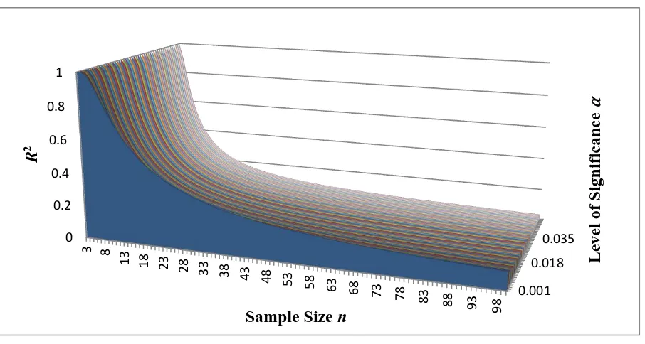
Figure 3 shows the power functions of R2 as a function of n and . As we can see, R2 displays a similar trait with regards to the sample size n, for all the different values of .
0 20 40 60 80 100 120
0 0.1 0.2 0.3 0.4 0.5 0.6 0.7 0.8 0.9 1
Sample
siz
e
n
R
2Critical
n
for each R
2given 3 values of
⍺
Figure 3. R2 as a function of n and ⍺
We found that this type of relationship between the R2, n, and the , is true even if we extend the size of n and increase the interval of values of . However, the values of the coefficients C1 and C2 will change accordingly. Thus, the obtained 200 different values of C1 and C2 for each individual are for the specific ranges of n and , mentioned above.
Table 2 shows a summary of the results of the coefficients C1 and C2 for selected values of .
Table 2. Values of the power functions’ coefficients C1 and C2
α C1 C2
0.001 4.3956 -0.791
0.01 4.3617 -0.900
0.02 4.2094 -0.939
0.03 4.0659 -0.963
0.04 3.9339 -0.980
0.05 3.8102 -0.995
0.1 3.2854 -1.042
0.15 2.8528 -1.072
0.2 2.4798 -1.093
We then ran regression models for the 200 values of each coefficient as a function of , and we obtained the following two models:
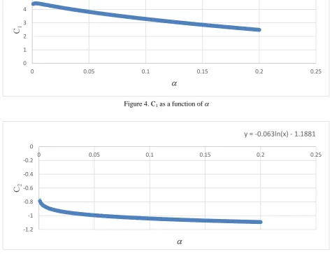
𝑪𝟏= (𝟒 𝟒𝟑𝟏𝟕)𝐞𝐱𝐩 (−𝟐 𝟗𝟑𝟖𝛂) (4)
𝑪𝟐= (−𝟎 𝟎𝟔𝟑) 𝐥𝐧() − 𝟏 𝟏𝟖𝟖𝟏 (5) For the interval of values considered, C1 is always positive and C2 is always negative:
C1 > 0 and C2 < 0
Thus, R2 can be expressed as a function of n and as follows:
𝑹𝟐 = [(𝟒 𝟒𝟑𝟏𝟕)𝐞𝐱𝐩 (−𝟐 𝟗𝟑𝟖𝛂)](𝒏)[(−𝟎 𝟎𝟔𝟑) 𝐥𝐧()−(𝟏 𝟏𝟖𝟖𝟏)] (6) Figures 4 and 5 show the relationships between C1 and C2 and .
0.001 0.018
0.035 0
0.2 0.4 0.6 0.8
1
3 8
13 18 23 28
33 38 43
48 53 58
63 68 73
78 83 88
93 98
Level of
Signif
ic
ance
⍺
R
2
Figure 4. C1 as a function of
Figure 5. C2 as a function of
In addition, this relationship determines the starting point of n for each alpha value, by making sure that R2 obtained is less than or equal to one. Therefore, given a level of significance , the developed model allows us to specify the lower bound of the sample size, and based on that, the lower bound of a significant R2. This determination can be accomplished by making sure that the starting point of n will provide a value of R2 that is less or equal to one, for the given . This is crucial, not only because it gives us a direct and straightforward relationship of R2 as a function of two known parameters, n and , but it also specifies the starting point of how big the sample size needs to be for every level of significance .
3.1.3 Model 1 Expansion: Significant Values of R2 - Multiple Regression Case
As we have mentioned before, this paper addresses the simple linear regression case. However, we have also included a glimpse of the future work we will be attempting to do when dealing with multiple dependent variables.
Equation (1) can be extended to the multiple regression case as follows:
𝐹 = [(𝑛 − 𝑘 − 1/𝑘)(𝑅2/(1 − 𝑅2))] , where 0 ≤ 𝑅2≤ 1, and 0 ≤ 𝐹 . Summary of the critical values:
o 𝑅2= 0 𝐹 = 0
o 𝑅2= 0 𝐹 = (𝑛 − 𝑘 − 1)/𝑘 o 𝑅2= 1 𝐹 =
y = (4.4317)exp(−2.938α)
0 1 2 3 4 5
0 0.05 0.1 0.15 0.2 0.25
C
1
y = -0.063ln(x) - 1.1881
-1.2 -1 -0.8 -0.6 -0.4 -0.2 0
0 0.05 0.1 0.15 0.2 0.25
C
2Even though the above analysis can be extended to multiple regression cases where k is the number of independent variables, the use of R2 and its interpretation is not as reliable.
In addition, the complexity of analyzing all the issues in multiple regression is beyond the scope of this paper and its targeted audience. Furthermore, when working with small samples, it is not advisable to keep adding predictors, as the gap between the R2 and the adjusted Ra2 will become more and more significant.
Table 3 shows the values of R2, for a multiple regression model with a particular alpha ( = 0.1) and different cases of independent variables k. The calculation was based on the assumption that with each additional independent variable, the sample size needs to be at least 50 + (8k). We realize that there are different relationships between the sample size and the number of independent variables, and we are not advocating that the one mentioned above is better or more accurate, but we simply chose it to show how the values of R2 would look, given an n and a k (for one particular value).
Table 3. Critical R2 values
n
k
1 2 3
58 0.5285 59 0.5241 60 0.5198 61 0.5156 62 0.5114 63 0.5073 64 0.5033 65 0.4993
66 0.4954 0.2313 67 0.4916 0.2285 68 0.4878 0.2258 69 0.4841 0.2231 70 0.4804 0.2206 71 0.4768 0.218 72 0.4732 0.2155 73 0.4697 0.2131
74 0.4663 0.2108 0.1808 75 0.4628 0.2084 0.1787 80 0.4465 0.1976 0.1689 90 0.4171 0.179 0.1522 100 0.3914 0.1636 0.1386
3.2 Model 2: Unexplained Variability Vs Total Variability – Simple Linear Regression
We will now look at the relationship between the standard deviation of the dependent variable y (Sy) and the standard error of the estimate (Se):
𝑆𝑒= 𝑆𝑦√((𝑛 − 1)/(𝑛 − 2)) ∗ (1 − 𝑅2) where 𝑆
𝑒= √(𝑆𝑆𝐸/(𝑛 − 2)) , 𝑆𝑦= √(𝑆𝑆𝑇/(𝑛 − 1)) and 𝑅2= 1 −
(𝑆𝑆𝐸/𝑆𝑆𝑇).
One way to look at whether the model (independent variable x) can contribute more to explaining the variability of y is by comparing the standard error of the estimate Se to the standard deviation of the y variable, Sy.
𝑆𝑒/𝑆𝑦≤ √((𝑛 − 1)/(𝑛 − 2)) .
Since n 3, and Se 0, the above inequality becomes:
0 ≤ 𝑆𝑒/𝑆𝑦≤ √2.
This shows that the standard error of the estimate, Se, can actually be bigger than the standard deviation of the dependent variable, Sy. But since we are dealing with significant models, we would like the independent variable to be able to explain better the variability of y, rather than looking just at the variability of y on its own; Se will then be smaller than Sy. Hence the amount √((𝑛 − 1)/(𝑛 − 2))(1 − 𝑅2) would be less than one.
This will result in the following:
𝑆𝑒/𝑆𝑦= √((𝑛 − 1)/(𝑛 − 2)) ∗ (1 − 𝑅2) 1 𝑦𝑖𝑒𝑙𝑑𝑠→ √((𝑛 − 1)/(𝑛 − 2)) ∗ (1 − 𝑅2) 1
((𝑛 − 1)/(𝑛 − 2)) ∗ (1 − 𝑅2) 1𝑦𝑖𝑒𝑙𝑑𝑠→ (𝑛 − 1) ∗ (1 − 𝑅2) 𝑛 − 2𝑦𝑖𝑒𝑙𝑑𝑠→ 𝑅2(−𝑛 + 1) −1 ,
which will give us the final simplified lower bound result of
𝑅2> 1/(𝑛 − 1). (7)
Even though this is a very safe lower bound to the actual significance values of R2, the interesting part of this relationship is that it is independent of alpha. Hence, these lower bound values will always be lower than any of the significant R2 regardless of what alpha we are considering. We double checked these results with all the significant R2 for all 200 values of .
Next, we compared these lower bounds to the significant R2 we obtained from our equation (6), and we confirmed that they are also lower than any values of R2 for any alpha.
3.2.1 Results of Model 2
Table 4 shows an example of the results by looking at a particular = 0.05. The first column displays the values of the critical R2 obtained from the critical test statistic F relationship, the second column contains the critical values from equation (6), and the third column contains the lower bound R2 values from equation (7).
Table 4. Comparing all the different critical R2
= 0.05
n Critical R2 (using F) R2 from (6) Lower bound R2 from (7)
5 0.7715 0.7660 0.2500
6 0.6584 0.6384 0.2000
7 0.5693 0.5473 0.1667
8 0.4995 0.4789 0.1429
9 0.4441 0.4257 0.1250
10 0.3993 0.3832 0.1111
11 0.3625 0.3484 0.1000
12 0.3318 0.3194 0.0909
13 0.3058 0.2948 0.0833
14 0.2835 0.2738 0.0769
15 0.2642 0.2555 0.0714
16 0.2474 0.2396 0.0667
17 0.2325 0.2255 0.0625
18 0.2193 0.2130 0.0588
19 0.2076 0.2018 0.0556
20 0.197 0.1917 0.0526
30 0.1304 0.1278 0.0345
40 0.0974 0.0959 0.0256
50 0.0777 0.0767 0.0204
60 0.0647 0.0639 0.0169
70 0.0554 0.0548 0.0145
80 0.0484 0.0480 0.0127
90 0.043 0.0426 0.0112
100 0.0387 0.0384 0.0101
Figure 6 shows all the boundaries of R2, the invalid area, the valid but insignificant area, and the significant area. The invalid one is the area below equation (7) lower bound values (grey area). The valid but insignificant area is the one between the lower bound graph and equation (6) values (orange area). Lastly, the significant area is the one above the significant curve depicted by equation (6) results (the rest of the graph).
Figure 6. Boundaries of R2
3.2.2 Model 2 expansion: Unexplained Variability vs Total Variability – Multiple Regression
As we have mentioned above, an attempt of dealing with multiple regression will be considered in future work. Below we look at the lower bound equation obtained when considering a value of k that is larger than one.
Se / Sy < 1 in 𝑆𝑒= 𝑆𝑦√[(𝑛 − 1)/(𝑛 − 𝑘 − 1)](1 − 𝑅2) implies that the amount √[(𝑛 − 1)/(𝑛 − 𝑘 − 1)](1 − 𝑅2) should be less than one. This results in
𝑅2> 𝑘/(𝑛 − 1). (8)
4. Concluding Remarks and Future Research Directions
There are several misconceptions when interpreting the values of the coefficient of determination, R2, in simple linear regression. In this paper, we comment on these observations and develop a relationship between the R2, n, and the level of significance α, for relatively small sample sizes. In addition, we develop a second model that serves as a lower bound to R2 as only a function of n. The idea behind this work is to have a better understanding of the connection between the different statistics used in linear regression, and to provide additional guidelines for the students, especially as they embark on their first statistics class.
More specifically, students in different fields, such as the Business schools, might not have a strong grasp on the mathematical concepts, nor do they take enough statistics classes to delve correctly into interpreting their software outcomes, yet, they are expected to use them in their academic career, and then later, when they join the workforce. Most importantly, in most cases, students when learning these concepts are not dealing with super-size samples, nor are they learning how to program models for big data, especially the ones that don’t have any programming background, yet require learning the basic concepts of statistics.
0 0.1 0.2 0.3 0.4 0.5 0.6 0.7 0.8 0.9
5 9 13 17 21 25 29 33 37 41 45 49 53 57 61 65 69 73 77 81 85 89 93 97
R
2
knowledge and skills in both the analytical and the programming part, yet they use statistical analysis for decision making.
Our focus in this paper is the small sample size data, and how the different values of R2 connect to the concept of “significance”. The main contribution of this research is to simplify these relationships, and present them in such a way, that any first-time user of basic statistics can have the ability of understanding the dos and don’ts of interpreting statistical results such as the R2 in a relatively small sample.
In order to do this, we developed two models. The first model is a power function: 𝑅2= 𝐶
1𝑛𝐶2 , where the coefficients C1 and C2 are functions of . It relates the coefficient of determination R2 to the sample size n, and the level of significance α. In addition, this relationship determines the starting point of n for each alpha value. This simplified relationship gives us the significant values of R2 for a range of specified values of n and α. In addition, this relationship determines the starting point of n for each alpha value.
The second model gives us a lower bound of R2 as only a function of the sample size n.
A future research direction is to extend this work to the multiple regression case with small number of independent predictors and to develop similar simplified relationships.
References
Bartko, J. J., Pulver, A. E., & Carpenter, W. T. (1988). The Power of Analysis: Statistical Perspectives. Part II, Psychiatry Research, 23, 301-309. https://doi.org/10.1016/0165-1781(88)90021-2
Bewick, V., Cheek, L., & Ball, J. (2003). Statistics Review 7: Correlation and Regression, BioMed central, 6(7), 451-459. https://doi.org/10.1186/cc2401
Bland, J. M., & Altman, D. G. (1996). Measurement Error and Correlation Coefficients, BMJ, 313-412. https://doi.org/10.1136/bmj.313.7048.41
Cohen, J. (1992). A Power Primer, Psychological Bulletin, 1(112), 155-159. https://doi.org/10.1037/0033-2909.112.1.155
Cramer, J. S. (1987). Mean and Variance of R2 in Small and Moderate Samples, Journal of Econometrics, 35, 253-266. https://doi.org/10.1016/0304-4076(87)90027-3
Erdfelder, E., Faul, F., & Buchner, A. (1996). GPOWER: A General Power Analysis Program, Behavior Research Methods, Instruments, and Computers, 28, 1-11. https://doi.org/10.3758/BF03203630
Filho, D. B. F., Paranhos, R., da Rocha, E. C., Batista, M., da Silva Jr, J. A., Santos, M. L. W. D., & Marino, J. G. (2013). When is Statistical Significance Not Significant? Brazilian Political Science Review, 1(7), 31-55. https://doi.org/10.1590/S1981-38212013000100002
Filho, D. B. F., Silva, J. A., & Rocha, E. C. (2011). What is R2 all About? Leviathan, 3, 60-68. https://doi.org/10.11606/issn.2237-4485.lev.2011.132282
Fisher, R. A. (1915). Frequency Distribution of the Values of the Correlation Coefficient in Samples from an Indefinitely Large Population, Biometrika, 4(10), 507-521. https://doi.org/10.2307/2331838
Fritz, M. S., & MacKinnon, D. P. (2007). Required Sample Size to Detect the Mediated Effect, Psychological Science, 3(18), 233-239. https://doi.org/10.1111/j.1467-9280.2007.01882.x
Gauss, C. F. (1809). Theoria motus corporum coelestium in sectionibus conicis solem Ambientum.
Hagquist, C., & Stenbeck, M. (1998). Goodness of Fit in Regression Analysis – R2 and G2 Reconsidered,” Quality and Quantity, 32, 229-245. https://doi.org/10.1023/A:1004328601205
Hsieh, F. Y., Bloch, D. A., & Larsen, M. D. (1998). A Simple Method of Sample Size Calculation for Linear and Logistic Regression, Statistics in Medicine, 17, 1623-1634.
https://doi.org/10.1002/(SICI)1097-0258(19980730)17:14<1623::AID-SIM871>3.0.CO;2-S
King, G. (1991). Stochastic Variation: A Comment on Lewis-Beck and Skalaban's the R-Square, Political Analysis, 2, 185-200. https://doi.org/10.1093/pan/2.1.185
Knofczynski, G. T., & Mundfrom, D. (2007). Sample Sizes when Using Multiple Linear Regression for Prediction, Educational and Psychological Measurement, 68, 431. https://doi.org/10.1177/0013164407310131
Legendre, A. M. (1805). Nouvelles méthodes pour la détermination des orbites des comètes, Paris: F. Didot.
McGraw, K. O., & Wong, S. P. (1996). Forming Inferences About Some Intraclass Correlation Coefficients, Psychological Methods, 1, 30-46. https://doi.org/10.1037/1082-989X.1.1.30
Moksony, F. (1999). Small is Beautiful. The Use and Interpretation of R2 in Social Research, Review of Sociology, (Special issue), pp.130-138.
Rodgers, J. L., & Nicewander, W. A. (1988). Thirteen Ways to Look at the Correlation Coefficient,” The American Statistician, 1(42), 59-66. https://doi.org/10.2307/2685263
Rovine, M. J., & Von Eye, A. (1997). A 14th Way to Look at a Correlation Coefficient: Correlation as the Proportion of Matches, The American Statistician, 1(51), 42-46. https://doi.org/10.1080/00031305.1997.10473586
Shrout, P. E., & Fleiss, J. L. (1979). Intraclass Correlations: Uses in Assessing Reliability, Psychological Bulletin, 86, 420-428. https://doi.org/10.1037/0033-2909.86.2.420
Copyrights
Copyright for this article is retained by the author(s), with first publication rights granted to the journal.