Generalised Lambda Distributions by Method of
Moments and Maximum Likelihood using the JSE-ASI
Returns
Peterson Owusu Junior (Corresponding author) Institute of Distance Learning (IDL)
Kwame Nkrumah University of Science & Technology (KNUST) PMB Kumasi, Ghana
Tel: 233-260-006-397 E-mail:[email protected]
Carl H. Korkpoe
Department of Computer Science, School of Physical Sciences University of Cape Coast, PMB Cape Coast, Ghana Tel: 233-543-179-583 E-mail: [email protected]
Received: Feb. 10, 2017 Accepted: April 5, 2017 Published: June 1, 2017 doi:10.5296/ajfa.v9i1.10913 URL: http://dx.doi.org/10.5296/ajfa.v9i1.10913
Abstract
1. Introduction
Risk is important to investors for any level of market return. In frontier markets with short histories, long historical data may be lacking for modeling purposes. Market analysts are also absent in most cases to follow usually thinly traded equities to serve the investor community. This makes it extra challenging for investors to assess the risk-return characteristics of their portfolios in such markets.
We seek to ameliorate this challenge by providing a flexible four-parameter distribution model; the Generalised Lambda Distribution (GLD) to model the characteristics of market returns and the tails risk essential to guide market participants in forming efficient portfolios. In the process of comparing the better fit between the GMM and MLE under GLD we show the performance of our models by comparing them to the two-parameter normal distribution; a popular but rather discredited model in risk modeling of equity returns (see Fama & MacBeth, 1973; Giot & Laurent, 2004; Hull & White, 1998).
Modeling market returns by using the normal distribution does not provide the flexibility needed as compared to, for instance, the four-parameter generalised lambda distribution. To capture the stylised facts of a security or a return series there arises the need to model the returns in their entirety. Value-at-Risk (VaR) vis-a-vis Expected Shortfall (ES), as good examples, requires us to capture the risk properties of a return using only the quantile values in the left tail of the distribution.
The need to model just the tail behaviour of the losses in assets returns is a matter of empirical concern. But is it well known that the normal distribution is a poor model for stock returns (Eberlein & Keller, 1995). The classes of generalised hyperbolic distribution (GHD) have the capabilities of mirroring both tail behaviour and asymmetries of returns which is a desired property of distributions in finance. Besides the normal distribution many models have been investigated (see Eberlein & Keller, 1995) but it was the class of hyperbolic distributions which turned out to be an excellent candidate to provide a more realistic model. In this paper we model the Johannesburg Stock Exchange All Share Index (JSE - ASI) with the generalised lambda distribution (GLD) using the generalised method of moments (GMM) and the maximum likelihood estimation (MLE) approaches to establish the better fit for the data.
Except for Corrado (2001), Tarsitano (2004), Chalabi, Scott, & Wuertz (2012), and Pfaff, (2013) there has been little application of GHD; especially of the generalised lambda distribution (GLD) to data. Pfaff (2013) for instance, applies the GHD and its special cases, namely; hyperbolic distribution (HYP), normal inverse Gaussian distribution (NIG), and generalised lambda distribution (GLD) to financial market data; the Hewlett-Packard (HWP), to draw useful insights.
for the DOW. We have, however, not seen these distributions in empirical work in emerging and frontier markets. Given investors perception that these two markets are risky (see Claessens, Dasgupta, & Glen, 1995; Errunza & Padmanabhan, 1988; Hassan, Maroney, El-Sady, & Telfah, 2003; Hearn, Piesse, & Strange, 2010); the need arises to establish risk-return characteristics in equity and indeed related securities in these markets on a sound theoretical footing. In this paper, therefore, we find the better fit for log returns of the Johannesburg Stock Exchange All Share Index (JSE-ASI) between the GMM and MLE methods.
2. Theoretical Framework
2.1 Generalised Hyperbolic Distributions (GHD)
Hyperbolic distributions are characterised by their log-density being a hyperbola unlike normal distributions whose log-density is a parabola. One can then expect to obtain a reasonable alternative for heavy tail distribution (Eberlein & Keller, 1995). The parameterised hyperbolic density function can be given as
ℎ ( ) = −
2 Κ − exp − + ( − ) + ( − ) (2.1)
where Κ is the modified Bessel function of the third kind with index Ι. and with > 0
and 0 ≤ | | < determine the shape of the distribution, while and are scale and location parameters respectively. Koudou & Ley (2014) assert that in 1977 Barndorff-Nielsen and Halgreen showed that the generalised inverse Gaussian distribution (GIGD), sometimes called Halphen Type A distribution, with the following probability density function
( ; , , ) = ( / )
/
2Κ exp −
1
2( + ) , ( > 0) (2.2)
has the property of infinite divisibility which is used in the representation of hyperbolic distributions as a mixture of normals. Any mixture of the r-dimensional normal distributions
( , Σ) determined by setting = + Δ and Σ = Δ. This class of mixtures includes the r-dimensional hyperbolic distribution
( , , , Δ) − + ( − )Δ ( − ) + (( − )) (2.3)
where Δ is a positive definite × matrix with determinant |Δ| = 1 and setting κ = − Δ , the norming constant is given by
( , , , Δ) = 1 (2 )( )/ .
κ( )/
2 ( )/ Κ
was introduced by the same authors a year earlier (Barndorff-Nielsen, Blaesild, & Halgreen, 1978; O. Barndorff-Nielsen & Halgreen, 1977).
Based on the daily prices of the 30 DAX shares over a three-year period Eberlein & Keller (1995) investigated the distributional form of compound returns after performing a number of statistical tests to the logical conclusion that some standard assumptions could not be justified. Hence, they introduced the class of hyperbolic distributions which can be fitted to empirical returns with high accuracy. This was the application of GHD to the increments of financial market price processes probably first proposed by Eberlein and Keller in 1995 (i.e. the returns resulting from geometric Brownian motion are increments of a Brownian motion process, thus are independent and normally distributed). Again tests applied to real data in this way demonstrate failure of the normality assumption.
The popularity of the class of GHDs in finance was pioneered in seminal papers in the late 1990s (see (Barndorff-Nielsen & Shephard, 1998; Barndorff-Nielsen & Halgreen, 1977; Eberlein, Keller, & Prause, 1998; Prause, 1997, 1999). However the application of hyperbolic distributions in fields other than finance is not limited. The motivation for Barndorff-Nielsen & Halgreen (1977) to introduce the hyperbolic distributions was the observation by Bagnold (1941) that the logarithm of the density function of distribution of the logarithm of the grain size in natural sand deposits looks more like a hyperbola than a parabola (Sørensen, 2006).
2.2 Generalised Lambda Distribution (GLD)
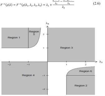
The four-parameter (quantile) GLD family is known for its high flexibility, producing distributions with a range of different shapes. To start with (Ramberg & Schmeister, 1974) show six regions in which the shape parameters can lie for which the shapes of the GLD are similar, as shown in Figure 1; the figure is as given in King & MacGillivray (1999) with notation introduced by Ramberg, Dudewicz, Tadikamalla, & Mykytka (1979), Chalabi et al. (2012), and Chalabi, Scott, & Würtz (2010). The modern Freimer, Kollia, Mudholkar, & Lin (1988) - FMKL GLD (2.6) places the only restriction of > 0. The fundamental motivation for the development of FMKL GLD is that the distribution is defined over all and (Su, 2007b).
The quantile probability density function of the GLD (henceforth referred to as RS GLD) is given as the inverse distribution function of Tukey’s lambda distribution (TLD)
( | ) = ( | , , , ) = + − (1 − ) (2.5)
where are the probabilities, ∈ [0,1], , are the location and scale parameters, and
, are the shape parameters jointly related to the strengths of the lower and upper tails, respectively. The original one-parameter TLD results in the limiting case = 0 and
( | ) = ( | , , , ) = + − ( )
(2.6)
Figure 1. Graph of the parameters regions of the GLD in the vs. space that produce proper statistical distributions. Source: (Chalabi et al., 2010)
The parameter constellations that fall in the third quadrant imply skewed and heavy-tailed distributions; that is a nice characteristic of stylised facts about financial return series giving more credence to the use of non-normal distributions, in this case GLD to capture this behaviour (Pfaff, 2013).
The various methods for estimation of the optimal values for the parameter vector in the literature include, among others (1) moment-matching approach by Ramberg & Schmeister (1974) and Ramberg et al. (1979), (2) percentile-based approach by Karian & Dudewicz (1999), (3) histogram-based approach by Su (2005), (4) goodness-of-fit approach by Owen (1988), (5) maximum likelihood (ML) and maximum spacing approaches by Cheng & Amin (1983) and Ranneby (1984) and (6) least squares (LS)-approach (see Karvanen & Nuutinen, 2008; Öztürk & Dale, 1982, 1985).
Stemming from an extensive investigation by Karian & Dudewicz (2000), King & MacGillivray (1999), Ramberg & Schmeister (1974), Ramberg et al. (1979), etc. on the symmetry distribution version of the GLD given for = , not all parameter combinations yield valid density functions (Pfaff, 2013). The probability density function of the GLD at
= ( | ) is given by
( ) = ( ( | )) =
− (1 − ) (2.7)
Valid parameter combinations of must yield (2.8) and (2.9):
( ) ≥ 0 (2.8)
( ) = 1 (2.9)
for ( ) in (2.7) to qualify as density function (Pfaff, 2013).
This is going to be the only mention of symmetry in this paper since the focus is fitting the GLD to financial return series. The limitation pointed out here does not affect the superiority of the GLD over normal distribution, at least, in fitting the JSE-ASI.
One advantage of the GLD is that the computation of VaR and ES can easily be achieved after a return series has been fitted herewith; expressed as positive numbers of returns and not for losses (Pfaff, 2013).
Hyperbolic distributions are characterised by their log-density being a hyperbola unlike normal distributions whose log-density is a parabola. One can then expect to obtain a reasonable alternative for heavy tail distribution (Eberlein & Keller, 1995). The parameterised hyperbolic density function can be given as
ℎ ( ) = −
2 Κ − exp − + ( − ) + ( − ) (2.2)
where Κ is the modified Bessel function of the third kind with index Ι. and with > 0
and 0 ≤ | | < determine the shape of the distribution, while and are scale and location parameters respectively. Koudou & Ley (2014) assert that in 1977 Barndorff-Nielsen and Halgreen showed that the generalised inverse Gaussian distribution (GIGD), sometimes called Halphen Type A distribution, with the following probability density function
( ; , , ) = ( / ) /
2Κ exp −
1
2( + ) , ( > 0) (2.2)
has the property of infinite divisibility which is used in the representation of hyperbolic distributions as a mixture of normals. Any mixture of the r-dimensional normal distributions
( , , , Δ) − + ( − )Δ ( − ) + (( − )) (2.3)
where Δ is a positive definite × matrix with determinant |Δ| = 1 and setting κ = − Δ , the norming constant is given by
( , , , Δ) = 1 (2 )( )/ .
κ( )/
2 ( )/ Κ
( )/ ( ) (2.4)
was introduced by the same authors a year earlier (Barndorff-Nielsen, Blaesild, & Halgreen, 1978; O. Barndorff-Nielsen & Halgreen, 1977).
3. Methodology
In comparing MLE and GMM we are embarking on a journey of goodness of fit. Thus going through parameter estimation procedure to find the values of GMM and MLE that best fit the JSE-ASI data. The GMM and MLE have come head-to-head as alternatives to statistical estimation since over two decades after the former was introduced in 1894 by Karl Pearson. In recent years, however, financial econometricians have found working under assumed likelihood functions restrictive, and have suggested using a generalised version of Pearson’s MM approach, commonly known as GMM estimation procedure as advocated by Bera & Bilias (2002) and Hansen (1982).
Fisher (1922) asserts that the parameters of the MM are those of an infinite population of the specified type having the same moments as those calculated from the sample, its application has not been shown except in the case of the normal curve. To discover whether this approximation is good or bad he proposes an improvement, if possible, by requiring a more adequate criterion. By assessing the suggestions from Fisher (1922), Pearson (1936) found that the additional computing work after the determination by moments is “as long as, I think longer than, the first fitting by moments”. The blunders in both MM and MLE are explored in the same paper thereof. Notwithstanding, GMM is seen, largely, as an applicable parameter estimation strategy which shells the classic method of moments, linear regression, and maximum likelihood (Chaussé, 2010, 2012).
3.1 Generalised Method of Moments (GMM)
The GMM is relatively advantageous for time series data. This comes as no surprise for the reason that Hansen (1982) introduced the GMM primarily with time series applications in mind, and it can be used to obtain parameter estimators that are consistent under weak distributional assumptions (Wooldridge, 2001). The method of moments consists of equating empirical moments with theoretical moments Focardi & Fabozzi (2004) in order to get estimators of the parameters (Iacus, 2011).
Chaussé (2010) and Chaussé (2012) thus conclude; because GMM depends only on moment conditions, it is a reliable estimation procedure for many models in economics and finance. With the right moment conditions the GMM is more appropriate than maximum likelihood. In this paper we see how that plays out for our set of data; a corroboration.
Further, in finance, there is no satisfying parametric distribution which reproduces the properties of stock returns except that the family of stable distributions is a good candidate. In this regard only the densities of the normal, Cauchy, and Levy distributions have a closed form expression (Chaussé, 2010).
The mathematical narrative that follows is based on Chaussé (2010). We would want a vector of parameters ∈ ℝ based on × 1 vector of unconditional moments below:
[ ( , )] = 0 (3.0)
where is vector of cross-sectional data, time series, or both. has to be the unique solution to (3.0) and be an element of a compact space for GMM to produce consistent estimates. Higher boundary conditions of ( , ) are also needed.
Given the linear model (3.1) in ( × 1) and ( × 1) matrices:
= + (3.1)
The most common method of estimating the parameter is least squares (LS) approach by solving || || hence the solution to the first order condition:
1 ⊺
( ) = 0 (3.2)
Equation (3.1) is the estimate of the moment condition of:
, ( ) = 0 (3.3)
( )
= 0 (3.4)
given that ( ) is the density of (Baum, Schaffer, & Stillman, 2003; Baum et al., 2003; Baum, Schaffer, Stillman, & others, 2007; Hansen, 1982; Hansen, Heaton, & Yaron, 1996; Stock, Wright, & Yogo, 2002). A lot of estimation methods including LS, ML, or instrumental variables (IV) can also be seen as being based on such moment conditions as in (3.2), therefore, they are special cases of GMM (Chaussé, 2010, 2012).
The moment condition is obtained by equating the derivatives of a log-likelihood to zero that MLE can be given an MM interpretation as well; (see Chaussé, 2010, 2012) for the relationships between GMM and IV, generalised LS, and ML, and pseudo-ML. Generally, the moment conditions [ ( , )] = 0 (3.0) is a vector of non-linear functions of the parameter with the number of unlimited by the same parameter (Chaussé, 2010, 2012). It is, therefore, a step in the right direction to estimate the parameters on GLD by GMM as well as MLE in this paper. In order to reduce the possibility of inefficiency there is the need to increase the number of instruments which is often greater than rendering (3.5) with no solution.
̅( ) =1 ( , ) = 0 (3.5)
Remedial methods for this situation are offered by Hansen (1982), with so-called two-stage GMM (2SGMM) in the original version of GMM, also Andrews (1991) and Newey & West (1987) with a heteroscedasticity and autocorrelation consistent (HAC)-like matrix. Further improvement to the properties of 2SGMM by Hansen et al. (1996) are the iterative 2SGMM (IT2SGMM) and the continuous updated estimator.
Like the MLE, GMM estimators are easily consistent, however, efficiency bias depend on the choice of moment conditions (Chaussé, 2010). Though the distribution-free feature of GMM gives a very good appeal, it is as good as its moment conditions.
3.2 Maximum Likelihood Estimation (MLE)
Unlike least-squares estimation which is primarily a descriptive tool, MLE is a preferred method of parameter estimation in statistics and it’s an indispensable tool for many statistical modelling techniques, in particular non-linear modeling with non-normal data (Myung, 2003). Out of two possible general approaches to fitting GLD to data, according to Su (2007a); using the discretised method and a definite fit to the data set such as maximising the goodness of fit, the MLE is usually the preferred method (see King & MacGillivray, 1999).
Let ( | ) denote the probability density function (PDF) that specifies the probability of observing vector given the parameter . The likelihood function can be given as:
( | ) = ( | ) (3.6)
For computational convenience the MLE estimate is obtained by maximising the log-likelihood function Myung (2003) so that the product (3.2) is transformed into a sum. Since the logarithm is an increasing function, maximising the likelihood or the log-likelihood gives the same results
(Focardi & Fabozzi, 2004). If the sample is IID then the likelihood is the product of individual likelihoods:
( | ) = ( | ) (3.7)
Assuming the log-likelihood function ( | ), is differentiable, if (MLE estimate) exists, it must satisfy the following partial differential equation called the likelihood equation:
( | )
= 0 (3.8)*
Equation (3.3) is only a necessary condition for the existence of MLE estimates. A sufficient condition requires that ( | ) is a maximum and not minimum. Hence the shape of the function be convex. Again from calculus (3.4) below must be true for = 1,2, … , .
( | )
< 0 (3.8)
For further reading see (Myung 2003; Iacus 2011).
In estimating the parameters of GLD the gld and GLDEX packages in R were employed. It is necessary to obtain quantiles, under the RS or FMKL for every observation , for
likelihood equations (3.9) and (3.10) below:
=
+ (1 − ) (3.9)
=
+ (1 − ) (3.10)
The key is to maximise the likelihood in (3.5) and (3.6); this can be done through the Nelder-Simplex algorithm (Su, 2007b). The MLE estimates can be heavily biased but asymptotically consistent, efficient, and unbiased for adequately large sample size (Iacus, 2011).
4. Data and Terminology
The price series of the JSE-ASI is collected daily from January 02, 2003 to December 31, 2015 giving a total of three thousand two hundred and fifty-two data points. The log return series of the JSE - ASI was calculated as:
= ln(1 + ) = ln ( ) − ln ( ) (3.11)
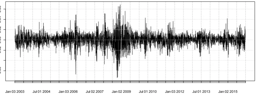
where is the continuously compounded return (natural logarithm of the simple gross return of an asset). According to Tsay (2010), statistical properties of log returns are more tractable. For average investors, returns is a complete scale-free summary of investment prospect. Campbell et al. (1998) also showed that returns have more attractive statistical properties such as stationarity and ergodicity. A time series plot of the returns is show in Figure 2.
Figure 2. A time series plot of the JSE - ASI returns from January 2003 to January 2015
Jan 03 2003 Jul 01 2004 Jan 03 2006 Jul 02 2007 Jan 02 2009 Jul 01 2010 Jan 03 2012 Jul 01 2013 Jan 02 2015
-0
.0
6
-0.
02
0
.00
0.
0
2
0.
04
0.
The time series plot exhibits two regimes - 2003 to 2009 and 2010 to 2015. In the first period the markets returns appeared more volatile particularly towards the end of the period in 2009. This is contrast to the period 2010 to 2015 when the market showed moderate volatility. Such behaviour in financial assets in the markets has been observed by previous researchers (Assoe, 1998; Chkili & Nguyen, 2014; Hamilton, 1989; M. R., 2001; van Norden & Schaller, 1993). Thus the statistical properties of the returns series will differ according to period. We therefore analysed the return series of the latter period of 2010 to 2015. Campbell, Lo, MacKinlay, & Whitelaw (1998) discuss at length the problem associated with using long-term horizon data series. Among others they posit the breakdown of the asymptotic inferences from such data. Most likely that may be due to what Hamilton (1989) identified as regime switching in the literature. We believe our data window more reflects the recent developments in the underlying economy which are transmitted to the market.
4.1 Testing for Classical Normality Assumptions
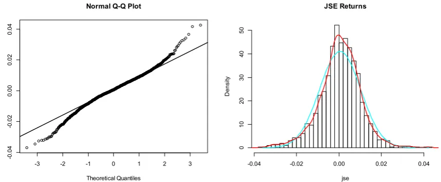
A test of the classical assumptions of normality looks at the first four moments of the distribution. The skewness and kurtosis show slight deviations from normality. The curve of the distribution is skewed to the left with fat-tails as the results show in the Table 1.
Table 1. Moments of the JSE - ASI returns from January, 2003 to January 2015
Mean Variance Skewness Kurtosis
0.0005 0.00009 -0.1701 1.4194
Figure 3. Q-Q plot and Normal distribution curve of the JSE - ASI returns from January, 2003 to January 2015
Finally in the Jarque-Bera and Cramer-von Mises normality tests; p-values respectively are nearly zero thus rejecting the null hypothesis of normality (Cromwell, Labys, & Terraza, 1994; D’Agostino, 1986). We were, therefore, able to reach the conclusion that the returns series of the JSE returns were not normally distributed.
4.2 Empirical Results from Methodology
From the above series of tests it is obvious the return series of the JSE All Share Index distribution shows marked departures from normality. We thus use the Generalized Lambda Distribution (GLD) to fit the entire distribution - the GLD not only models the tail behaviour but also the entirety of the return distribution (Pfaff, 2013). We used our selected method of moments and maximum likelihood estimation respectively.
4.3 Method of Moments
The estimated parameters of the Generalized Lambda Distribution using the method of moments are shown in Table 2.
Table 2: The four parameters GLD obtained from the JSE - ASI returns from January, 2003 to January 2015
λ1 λ2 λ3 λ4
0.072966 1.899254 -0.0288 0.00986
The parameters are the used to estimate the moments of the markets returns in Table 3.
-3 -2 -1 0 1 2 3
-0 .0 4 -0. 02 0. 0 0 0. 02 0. 04
Normal Q-Q Plot
Theoretical Quantiles S a m p le Q uant ile s JSE Returns jse De n sit y
-0.04 -0.02 0.00 0.02 0.04
Table 3. The four moments of GMM obtained from the JSE - ASI returns from January, 2003 to January 2015
Mean Variance Skewness Kurtosis
0.0522 0.9453 -0.1701 1.4193
These values compared to the moments from the normal distribution are almost the same. However a test of Kolmogorov-Smirnoff Distance (D) recommended by Su (2007b), gave the distance D = 0.97411 with a p-value of 0.1. This test has the null hypothesis that the sample data is drawn from the same distribution as the fitted distribution. With a p-value of 0.1, we fail reject the null hypothesis and conclude that the returns data came from the GLD using the method of moments.
4.4 Maximum Likelihood Method
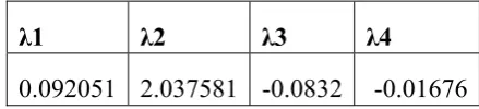
Parametrising the GLD using the maximum likelihood method we get the values as shown in the Table 4.
Table 4. The four parameters of the parameterised GLD obtained from the JSE - ASI returns from January, 2003 to January 2015
λ1 λ2 λ3 λ4
0.092051 2.037581 -0.0832 -0.01676
Using these parameters to compute the moments of the distribution we get Table 5.
Table 5. The four moments of the parameterised GLD obtained from the JSE - ASI returns from January, 2003 to January 2015
Mean Variance Skewness Kurtosis
0.055878 0.957247 -0.36028 2.520229
Figure 4. A histogram of the JSE - ASI returns from January, 2003 to January 2015 obtained by MM
Figure 5. A histogram of the JSE - ASI returns from January, 2003 to January 2015 obtained by MLE
From Figure 4 and Figure 5 it is clear that using the GLD with the method of moments gave a histogram that closely described the entire distribution. Though the maximum likelihood method fairly described the data, it comes at a further computational effort making the method of moments more suitable for the estimation period.
5. Conclusions
Measuring volatility accurately has become the preoccupation of financial institutions as it determines their survival in increasingly turbulent markets. For tail risk measures like value-at-risk (VaR) and expected tail loss (ETL), the correct distribution of the data is a first
Method of Moments Fit
Returns
De
n
si
ty
-4 -2 0 2 4
0
.00
.1
0
.20
.3
0
.40
.5
Method of Maximum Likelihood
JSE Returns
Dens
ity
-4 -2 0 2 4
0.
0
0
.1
0.
2
0
.3
0.
4
0
step. Markets have swung from end to end on the volatility spectrum so violently that the normal distribution no longer accurately describes the entire distribution nor gives the correct quantiles in the tails for risk management purposes.
We have demonstrated the use of the generalized lambda distribution as an alternative using the method of moments and maximum likelihood estimates in modeling the return series of the JSE All Share index. Overall both the method of moments and maximum likelihood methods describe fairly accurately the distribution of the returns.
However, the method of moments with the Kolmogorov-Smirnoff Distance good-of-fit statistics and the quantile-quantile graph provides a better fit to the data. We have provided a basis for estimating the tail events useful in risk and portfolio management on the Johannesburg Stock Exchange.
References
Andrews, D. W. K. (1991). Heteroskedasticity and Autocorrelation Consistent Covariance Matrix Estimation. Econometrica, 59(3), 817-858. https://doi.org/10.2307/2938229
Assoe, K. (1998). Regime-Switching in Emerging Stock Market Returns (SSRN Scholarly Paper No. ID 2631519). Rochester, NY: Social Science Research Network. Retrieved from http://papers.ssrn.com/abstract=2631519
Bagnold, R. A. (1941). The physics of wind blown sand and desert dunes. Methuen, London, 265(10).
Barndorff-Nielsen, O., Blaesild, P., & Halgreen, C. (1978). First hitting time models for the generalized inverse Gaussian distribution. Stochastic Processes and Their Applications, 7(1), 49-54. https://doi.org/10.1016/0304-4149(78)90036-4
Barndorff-Nielsen, O. E., & Shephard, N. (1998). Aggregation and model construction for volatility models. Nuffield College. Retrieved from http://www.nuff.ox.ac.uk/economics/papers/1998/w7/ECON.PDF
Barndorff-Nielsen, O., & Halgreen, C. (1977). Infinite divisibility of the hyperbolic and generalized inverse Gaussian distributions. Zeitschrift Für Wahrscheinlichkeitstheorie Und Verwandte Gebiete, 38(4), 309-311. https://doi.org/10.1007/BF00533162
Baum, C. F., Schaffer, M. E., & Stillman, S. (2003). Instrumental variables and GMM: Estimation and testing. Stata Journal, 3(1), 1-31.
Baum, C. F., Schaffer, M. E., Stillman, S., & others. (2007). Stata module for extended instrumental variables/2SLS, GMM and AC/HAC, LIML and k-class regression. Boston College Department of Economics, Statistical Software Components S, 425401, 2007.
financial markets. Macroeconomic Dynamics, 2(04), 559-562.
Chalabi, Y., Scott, D. J., & Wuertz, D. (2012). Flexible distribution modeling with the generalized lambda distribution. Retrieved from https://mpra.ub.uni-muenchen.de/43333/ Chalabi, Y., Scott, D. J., & Würtz, D. (2010). The generalized lambda distribution as an alternative to model financial returns. Working paper, Eidgenössische Technische Hochschule and University of Auckland, Zurich and Auckland. Retrieved from https://www.rmetrics.org/sites/default/files/glambda_0.pdf
Chaussé, P. (2010). Computing Generalized Method of Moments and Generalized Empirical Likelihood with R. Journal of Statistical Software, 34(i11). Retrieved from https://ideas.repec.org/a/jss/jstsof/34i11.html
Chaussé, P. (2012). Generalized empirical likelihood for a continuum of moment conditions. Retrieved from http://www.archipel.uqam.ca/4653
Cheng, R. C. H., & Amin, N. A. K. (1983). Estimating parameters in continuous univariate distributions with a shifted origin. Journal of the Royal Statistical Society. Series B (Methodological), 394-403.
Chkili, W., & Nguyen, D. K. (2014). Exchange rate movements and stock market returns in a regime-switching environment: Evidence for BRICS countries. Research in International Business and Finance, 31(C), 46-56.
Claessens, S., Dasgupta, S., & Glen, J. (1995). Return Behavior in Emerging Stock Markets. The World Bank Economic Review, 9(1), 131-151.
Corrado, C. J. (2001). Option pricing based on the generalized lambda distribution. Journal
of Futures Markets, 21(3), 213-236.
https://doi.org/10.1002/1096-9934(200103)21:3<213::AID-FUT2>3.0.CO;2-H
Cromwell, J. B., Labys, W. C., & Terraza, M. (1994). Univariate tests for time series models. Sage Publications.
D’Agostino, R. B. (1986). Goodness-of-Fit-Techniques. CRC Press.
Eberlein, E., & Keller, U. (1995). Hyperbolic distributions in finance. Bernoulli, 1(3), 281-299. https://doi.org/10.3150/bj/1193667819
Eberlein, E., Keller, U., & Prause, K. (1998). New insights into smile, mispricing, and value at risk: The hyperbolic model*. The Journal of Business, 71(3), 371-405.
Errunza, V. R., & Padmanabhan, P. (1988). Further evidence on the benefits of portfolio investments in emerging markets. Financial Analysts Journal, 44(4), 76-78.
Fama, E. F., & MacBeth, J. D. (1973). Risk, Return, and Equilibrium: Empirical Tests. Journal of Political Economy, 81(3), 607-636.
Engineering Sciences, 222(594-604), 309-368. https://doi.org/10.1098/rsta.1922.0009
Focardi, S. M., & Fabozzi, F. J. (2004). The Mathematics of Financial Modeling and Investment Management. Hoboken, New Jersey: John Wiley & Sons, Inc.
Freimer, M., Kollia, G., Mudholkar, G. S., & Lin, C. T. (1988). A study of the generalized Tukey lambda family. Communications in Statistics-Theory and Methods, 17(10), 3547-3567. Giot, P., & Laurent, S. (2004). Modelling daily value-at-risk using realized volatility and ARCH type models. Journal of Empirical Finance, 11(3), 379-398.
Hamilton, J. D. (1989). A new approach to the economic analysis of nonstationary time series and the business cycle. ECONOMETRICA, 57(2), 357-384.
Hansen, L. P. (1982). Large Sample Properties of Generalized Method of Moments Estimators. Econometrica, 50(4), 1029-1054. https://doi.org/10.2307/1912775
Hansen, L. P., Heaton, J., & Yaron, A. (1996). Finite-Sample Properties of Some Alternative GMM Estimators. Journal of Business & Economic Statistics, 14(3), 262-280. https://doi.org/10.1080/07350015.1996.10524656
Hassan, M. K., Maroney, N. C., El-Sady, H. M., & Telfah, A. (2003). Country risk and stock market volatility, predictability, and diversification in the Middle East and Africa. Economic Systems, 27(1), 63-82.
Hearn, B., Piesse, J., & Strange, R. (2010). Market liquidity and stock size premia in emerging financial markets: The implications for foreign investment. International Business Review, 19(5), 489-501.
Hull, J. C., & White, A. D. (1998). Value at Risk When Daily Changes in Market Variables are not Normally Distributed. The Journal of Derivatives, 5(3), 9-19. https://doi.org/10.3905/jod.1998.407998
Iacus, S. M. (2011). Option Pricing and Estimation of Financial Models with R (1st ed.). West Sussex, PO19 8SQ, United Kingdom: John Wiley & Sons, Ltd.
Karian, Z. A., & Dudewicz, E. J. (1999). Fitting the generalized lambda distribution to data: a method based on percentiles. Communications in Statistics - Simulation and Computation, 28(3), 793-819. https://doi.org/10.1080/03610919908813579
Karian, Z. A., & Dudewicz, E. J. (2000). Fitting Statistical Distributions: The Generalized Lambda Distribution and Generalized Bootstrap Methods. CRC Press.
Karvanen, J., & Nuutinen, A. (2008). Characterizing the generalized lambda distribution by L-moments. Computational Statistics & Data Analysis, 52(4), 1971-1983.
Surveys, 11, 161-176. https://doi.org/10.1214/13-PS227
M. R., H. (2001). A Regime-SWITCHING MODEL OF LONG-TERM STOCK RETURNS. NORTH AMERICAN ACTUARIAL JOURNAL, 5(2).
Myung, I. J. (2003). Tutorial on maximum likelihood estimation. Journal of Mathematical Psychology, 47(1), 90-100.
Newey, W., & West, K. (1987). A Simple, Positive Semi-definite, Heteroskedasticity and Autocorrelation Consistent Covariance Matrix. Econometrica, 55(3), 703-08.
Owen, A. B. (1988). Empirical likelihood ratio confidence intervals for a single functional. Biometrika, 75(2), 237-249. https://doi.org/10.1093/biomet/75.2.237
Öztürk, A., & Dale, R. F. (1982). A Study of Fitting the Generalized Lambda Distribution to Solar Radiation Data. Journal of Applied Meteorology, 21(7), 995-1004. https://doi.org/10.1175/1520-0450(1982)021<0995:ASOFTG>2.0.CO;2
Öztürk, A., & Dale, R. F. (1985). Least squares estimation of the parameters of the generalized lambda distribution. Technometrics, 27(1), 81-84.
Pearson, K. (1894). Contributions to the Mathematical Theory of Evolution. Philosophical Transactions of the Royal Society of London A: Mathematical, Physical and Engineering Sciences, 185, 71-110. https://doi.org/10.1098/rsta.1894.0003
Pearson, K. (1936). Method of Moments and Method of Maximum Likelihood. Biometrika, 28(1/2), 34-59. https://doi.org/10.2307/2334123
Pfaff, B. (2013). Financial Risk Modelling and Portfolio Optimization with R. West Sussex, PO19 8SQ, United Kingdom: John Wiley & Sons Ltd.
Prause, K. (1997). Modelling financial data using generalized hyperbolic distributions. fDM
Preprint, 48. Retrieved from
http://citeseerx.ist.psu.edu/viewdoc/download?doi=10.1.1.416.1199&rep=rep1&type=pdf Prause, K. (1999). The generalized hyperbolic model: Estimation, financial derivatives, and
risk measures. Citeseer. Retrieved from
http://citeseerx.ist.psu.edu/viewdoc/download?doi=10.1.1.382.9958&rep=rep1&type=pdf Ramberg, J. S., Dudewicz, E. J., Tadikamalla, P. R., & Mykytka, E. F. (1979). A probability distribution and its uses in fitting data. Technometrics, 21(2), 201-214.
Ramberg, J. S., & Schmeister, B. W. (1974). An approximate method for generating asymmetric random variables. Communication of the ACM, 17, 78-82.
Ranneby, B. (1984). The maximum spacing method. An estimation method related to the maximum likelihood method. Scandinavian Journal of Statistics, 93-112.
Sørensen, M. (2006). On the size distribution of sand. Unpublished Paper,Department of Applied Mathematics and Statistics University of Copenhagen Universitetsparken 5, DK-2100 Copenhagen Ø, Denmark, 10.
Stock, J., Wright, J., & Yogo, M. (2002). A Survey of Weak Instruments and Weak Identification in Generalized Method of Moments. Journal of Business & Economic Statistics, 20, 518-529.
Su, S. (2005). A Discretized Approach to Flexibly Fit Generalized Lambda Distributions to Data. Journal of Modern Applied Statistical Methods, 4(2). Retrieved from http://digitalcommons.wayne.edu/jmasm/vol4/iss2/7
Su, S. (2007a). Fitting single and mixture of generalized lambda distributions to data via discretized and maximum likelihood methods: GLDEX in R. Journal of Statistical Software, 21(9), 1-17.
Su, S. (2007b). Numerical Maximum Log Likelihood Estimation for Generalized Lambda Distributions. Comput. Stat. Data Anal., 51(8), 3983-3998. https://doi.org/10.1016/j.csda.2006.06.008
Tarsitano, A. (2004). Fitting the generalized lambda distribution to income data (pp. 1861-1867). Presented at the In COMPSTAT’2004 Symposium.
Tsay, R. S. (2010). Analysis of Financial Time Series (Third Edition). Hoboken, New Jersey: John Wiley & Sons, Inc.