Issues
ISSN: 2146-4138
available at http: www.econjournals.com
International Journal of Economics and Financial Issues, 2016, 6(2), 653-659.
Estimation of Private Consumption Function of Iran:
Auto-regressive Distributed Lag Approach to Co-integration
Behnam Nikbin
1*, Saman Panahi
21Allameh Tabataba’i University, Tehran, Iran, 2Allameh Tabataba’i University, Tehran, Iran. *Email: [email protected]
ABSTRACT
Considering consumption due to its pivotal role in economic growth and also aggregate demand and specially its long-run analysis have always been in the center of attention. In this study, we have estimated private consumption function, using auto-regressive distributed lag (ARDL) approach and employing annual data during 1978-2012. Short-run elasticity of private consumption function regarding to its lag is 0.50 and to gross domestic product is approximately 0.56. Also, the latter amount for long-run elasticity is 1.13. Furthermore, the estimation demonstrates a negative correlation between inflation and private consumption in both long-run and short-run relationships. Error correction model is estimated as well, and the coefficient is equal to −0.49 which shows the pace in which the private consumption function adjusts to its long-run equilibrium.
Keywords: Consumption Function, Auto-regressive Distributed Lag Approach, Error Correction Model
JEL Classifications: C13, C22, E21
1. INTRODUCTION
According to economics literature, consumption is defined as the goods and services purchased by households. By holding this definition, consumption is a key element and determinative variable in economic booms and recessions. Changes in consumers’ expenditure could be a source of economic shocks and also, marginal propensity to consume (MPC) is crucial for fiscal-policy multiplier (Manki , 2012. p. 465).
There is also an increasing evidence, which magnifies the importance of consumption studies in developing countries, especially the ones which are dependent on oil and oil revenues due to oil dichotomy; on the one hand, these countries have a poor agriculture sector and also labor-intensive which is lagged behind in comparison with the industrial sector, which is capital-intensive; on the other hand, oil acts as a double-edged sword, which reflect its negative behavior as the tendency of itself to foreign sectors and intensifies the distance between private sector and public sector. In such a kind of situation the necessity of paying attention to a suitable and also effici nt economic model considering the development plans is inevitable and undeniable. In this paper, we have estimated a consumption function for Iran, with respect to
the Friedman’s consumption function, by using auto-regressive distributed lag (ARDL) method and also we calculated the long-run and short-long-run elasticity of consumption.
2. EMPIRICAL STUDIES REVIEW
In one study entitled “How much do we care about absolute versus relative income and consumption?” with the aid of survey-experimental methods it has found that most individuals are concerned with both relative income and relative consumption of particular goods. The degree of concern varies in the expected direction depending on the properties of the good. However, it is also found that relative consumption is also important for vacation and insurance, which are typically seen as non-positional goods. Further, absolute consumption is also found to be important for cars and housing, which are widely regarded as highly positional (Alpizar et al., 2005).
constraints can account for two key patterns of consumption and asset holdings over the life cycle. First, consumption expenditures on both durable and non-durable goods are hump-shaped. Second, young households keep very few liquid assets and hold most of their wealth in consumer durables. Thus it is concluded that durables are a key feature to explain both the hump in consumption of durables and non-durables and the optimal asset allocation of households (Fernandez-Villaverde and Krueger, 2005).
In a research with the title of “The direct substitution between government and private consumption in East Asia” it is studied empirically the extent to which government consumption substitutes for private consumption in nine East Asia countries. Panel co-integrating regression uncovers a significantly positive elasticity of substitution between government and private consumption, implying on average government and private consumption are substitutes in East Asia. Country-by-country analysis, however, reveals diversity in the substitutability estimates. The four North East countries – China, Hong Kong, Japan, and Korea – tend to share similar and moderate values of the substitution elasticity. For the five ASEAN countries studied in this paper, the relationship between private and government consumption vary substantially, both in the sign and magnitude of the elasticity of substitution. Private and government consumption in Malaysia and Thailand are strong substitutes, but they are found to be complements in Indonesia and Singapore. In between is the Philippines which has a near zero elasticity of substitution (Kwan, 2006).
There are lots of studies have been made in Iran and the majority are fundamentally related to the “permanent income” theory of Friedman. In some researches consumption is divided into two whole segments, government and private consumption and also the latter is divided into both urban and rural sectors. This kind of segmentation is made considering both prominent role of oil in this country and the way of its usage which leads to inefficient oil revenues allocation and also “Fei-Ranis” issue which concentrates on the existence of a vast and noticeable agriculture sector but passive, along with an active and small industrial sector.
However, few works have been done about estimating consumption function in Iran. In one study with respect to Fei-Ranis conflict hypothesis, Iran’s consumption function is divided into two parts; First segment focuses on urban and rural sectors and the second category considers durable and non-durable goods.
Results demonstrate the higher explanatory power of Friedman’s consumption theory, comparing with Keynes, Duesenberry and Modigliani in the space of 1974-1998 in Iran.
The mentioned study which is made regarding to the first 5-year development plan, leaded to the fact that the long-run consumption curve passes through the origin of coordinates with a constant slope. Hence, MPC (in long-term) is constant and equal to average propensity to consume (Zarranejad, 2003).
A considerable amount of gross national product is dedicated to consumption expenditures, and also has a crucial role in macroeconometrics models.
Due to the dichotomy of oil which causes disequilibrium among government and private consumption behavior and also regarding to the traditional conflicts which results in a prominent distinction between urban and rural consumption behavior, three behavioral equations have been adopted to justify the existence of consumption in the model - urban consumption expenditure, rural consumption expenditure and government consumption expenditure. These equations are estimated using ordinary least squares (OLS) and two stages least squares methods (Arabmazar and Noferesti, 2006).
Another estimation and analysis has been made considering differing income deciles, with the aid of ARDL approach during 1982-2006; Results are illustrated a significant relationship between variables. Long-run MPC for low income group was equal to 0.97 and for high income ones was 0.66 and totally it is estimated 0.81. However, the short-run MPC was 0.55 (Fakhrai and Mansouri, 2008).
According to another study, private consumption function is estimated in order to attain both long-run and short-run MPC from 1959 to 2003, using ARDL method, which results indicated that MPC for both long- and short-terms are respectively, 0.49 and 0.37. And also, liquidity coefficient is 0.1 (as a proxy for real social wealth) and has a significant and positive effect on private consumption (Ahmad et al., 2008).
Another analysis on private consumption function for Iran is made, using the Engle–Granger two-step procedure for the timeframe of 1959-1995 and results have shown that long-run MPC is 0.76 and for short-run is 0.68 and the short-run dynamic is approximately 0.46 which reflectsthat 46% of disequilibrium between long-term and short-term consumption adjusts every year (Valadkhani, 1997).
3. LITERATURE REVIEW
The consumption function which is introduced for the firsttime by John Maynard Keynes in “general theory,” after the big recession in 1930, is often written as:
C = C0 + cY, C0 > 0, 0 < c < 1
Where, C is consumption, Y is disposable income, C0 is a constant, and c is the marginal propensity to consume (Mankiw, 2012. p. 466-467).
income is the key point of their theory.
Friedman by introducing the “permanent income” shows that the key element in private consumption behavior is permanent income. In this theory, permanent income is defined as the amount of annual fixed income which its present value is equal to household assets and expected income. To put it another way, permanent income is equivalent to average income of a few past years. Hence, Friedman mentioned that using relative income in permanent income theory, is inevitable due to two reasons. First of all, differing consumption-income regressions between different consumers in different countries, indicates diverse levels of living in societies. Secondly, distinctions in saving-to-income ratio indicates different types of behaviors.
Another important finding of Friedman, backs to his remarks on “adaptive expectations” to justify people behaviors. The discussion has entered a new phase by introducing the “rational expectations” under the works of Robert Hall. Hall investigates the differences among current income and consumption based on random walk hypothesis and believed that the only segment of permanent income which affects current consumption is transitory income. He also mentioned that a consumer is able to predict the current consumption (Ct) regarding to previous period’s consumption, if interest rate and given discount rate for the consumer are both (Ct−1) (based on rational expectation assumption) determined and vivid (Fakhrai and Mansouri, 2008).
Consumption and investment are important to both growth and fluctuations. With regard to growth, the division of society’s resources between consumption and various types of investment in physical capital, human capital, and research and development is central to standards of living in the long-run. That division is determined by the interaction of households’ allocation of their incomes between consumption and saving given the rates of return and other constraints they face, and firms investment demand given the interest rates and other constraints they face. With regard to flu tuations, consumption and investment make up the vast majority of the demand for goods. There are two other reasons for studying consumption and investment. First, they introduce some important issues involving fin ncial markets. Financial markets affect the macroeconomy mainly through their impact on consumption and investment. In addition, consumption and investment have important feedback effects on financia markets. Second, much of the most insightful empirical work in macroeconomics in recent decades has been concerned with consumption and investment (Romer, 2012).
Consider an individual who lives for T periods whose lifetime utility is:
U u C ut u
t T
= ′ • > ′′ • < =
∑
( ), ( ) , ( )1 0 0 (1)
Where, u(
•
) is the instantaneous utility function and Ct is consumption in period t. The individual has initial wealth of A0and labor incomes of Y1, Y2,…YT in the T periods of his or her life;
the individual takes these as given. The individual can save or
borrow at an exogenous interest rate, subject only to the constraint that any outstanding debt be repaid at the end of his or her life. For simplicity, this interest rate is set to 01 Thus the individual’s
budget constraint is:
Ct A Y
t T t t T = =
∑
≤ +∑
1 0 1 (2)
Since the marginal utility of consumption is always positive, the individual satisfies the budget constraint with equality. The Lagrangian for his or her maximization problem is therefore:
= + + − = = =
∑
∑
∑
u Ct A Yt Ct t T t T t T( ) λ 0
1 1
1 (3)
The first-order condition forCt is:
′ =
u C( )t λ (4)
Since (4) holds in every period, the marginal utility of consumption is constant. And since the level of consumption uniquely determines its marginal utility, this means that consumption must be constant. Thus C1 = C2 =…=CT. Substituting this fact into the
budget constraint yields:
C
T A Y
t t t T = + =
∑
1 01 for all t (5)
The term in brackets is the individual’s total lifetime resources. Thus (5) states that the individual divides his or her lifetime resources equally among each period of life. This analysis implies that the individual’s consumption in a given period is determined not by income that period, but by income over his or her entire lifetime. In the terminology of Friedman (1957), the right-hand side of (5) is p`1ermanent income, and the difference between current and permanent income is transitory income. Equation (5) implies that consumption is determined by permanent income. To see the importance of the distinction between permanent and transitory income, consider the effect of a windfall gain of amount Z in the first period of life. Although this windfall raises current income by Z, it raises permanent income by only Z/T. Thus if the individual’s horizon is fairly long, the windfall’s impact on current consumption is small. One implication is that a temporary tax cut may have little impact on consumption. Also it is completely possible to consider an analysis of consumption function under the uncertainty circumstances and regarding to interest rate (Romer, 2012).
Keynes proposed that consumption depends largely on current income. He suggested a consumption function of the form:
C = f (Yc) (6)
Where, Yc represents current income.
More recently, economists have argued that consumers understand that they face an intertemporal decision. Consumers look ahead to their future resources and needs, implying a more complex consumption function than the one Keynes proposed. This work suggests instead that:
C = f (Yc, W, Ye, r) (7)
Where, W is wealth, Ye represents expected earnings in the future
and r is the interest rate.
In other words, current income is only one determinant of aggregate consumption. Economists continue to debate the importance of these determinants of consumption. There remains disagreement about, for example, the influence of interest rates on consumer spending, the prevalence of borrowing constraints, and the importance of psychological effects. Economists sometimes disagree about economic policy because they assume different consumption functions. For instance, the debate over the effects of government debt is in part a debate over the determinants of consumer spending. The key role of consumption in policy evaluation is sure to maintain economists’ interest in studying consumer behavior for many years to come (Mankiw, 2012. p. 492).
Unlike the hypothesis of random walk, some studies demonstrate that, only unexpected policy changes can affect consumption, if consumers follow the permanent income hypothesis and consider rational expectations (Campbell and Mankiw, 1989).
4. DATA, METHODOLOGY AND
ESTIMATION
In this part we estimate the consumption function and also find the equilibrium relation between the main variables. In this investigation we employed annual data during 1978-2012 using the time series database of central bank of Iran (CBI, 2014). We use Microfit4.1 to estimate and analyze the estimation
General model which is used in this paper is the below function:
PCON = f (PCONt−1, GDP, P) (8)
Where, PCONt is total private consumption as explanatory variable along with its lag (PCONt−1), GDPt is the gross domestic product
and Pt is the inflation and εt is the error term. Hence, the desired equation would specify as a log-linear equation:
logPCONt = C0 + α1logPCONt−1 + α2logGDPt + α3Pt + εt (9)
Theoretically, we expect that α1<0 which means consumption
in period t and t-1 are correlated to each other directly and positively. Also α2< 0 and α3< 0. Before the estimation of model,
we can observe the strong long-run relationship between private consumption and gross domestic product (GDP) in the Figure 1.
Before the estimation, we must take the stationarity of variables into account, otherwise, we might face spurious regression. Once non-stationarity is introduced in 1970, first reactions to mitigate this issue was to use first order differences in order to make the series stationary. Although this method is statistically credible, but it can eliminate the long-run information as well (Soori, 2013. p. 492).
In general, economic relationships may be generated by an autoregressive distributed lag (ADRL) scheme. The simplest form is the ADRL (1,1) model which is given by:
Yt = α + λYt−1 + β0Xt + β1Xt−1 + ut (10)
Where, both Yt and Xt are lagged once. By specifying higher order lags for Yt and Xt, say an ADRL (p, q) with p lags on Yt and q lags on Xt, one can test whether the specification now is general enough to ensure white noise disturbances. Next, one can test whether some restrictions can be imposed on this general model, like reducing the order of the lags to arrive at a simpler ADRL model, or estimating the simpler static model with the Cochrane-Orcutt correction for serial correlation. This general to specific modeling strategy is prescribed by David Hendry and is utilized by the econometric software PC-Give.
Returning to the ADRL (1, 1) model in (10) one can invert the autoregressive form as follows:
Yt = α(1 + λ + λ2 +…) + (1 + λL + λ2L2 +…) (β
0X1 + β0Xt−1 + ut)
(11)
Provided |λ| < 1. This equation gives the effect of a unit change in Xt
on future values of Yt. In fact, ∂Yt/∂Xt = β0 while ∂Yt+1/∂Xt=β1+λβ0,
etc. This gives the immediate short-run responses with the long-run effect being the sum of all these partial derivatives yielding (β1 +
β0)/(1−λ). This can be alternatively derived from (10) at the long-run static equilibrium (Y*, X*) where Yt = Yt−1 = Y*, Xt = Xt−1 = X*,
and the disturbance is set equal to zero, i.e.,
Y* = X*
− +
+ − α
λ
β β
λ
1 1
1 0
Replacing Yt by Yt−1+∆Yt and Xt by Xt−1 + ∆Xt in (10) one gets:
∆Yt = α + β0∆Xt – (1−λ)Yt–1 + (β0 + β1)Xt−1 + ut (12)
This can be rewritten as:
∆ = ∆ − − −
− − +
− +
− −
Yt β Xt λ Yt α Xt u
λ
β β
λ
0 (1 )[ 1 1 10 1 1]
(13)
Note that the term in brackets contains the long-run equilibrium parameters derived in (12). In fact, the term in brackets represents the deviation of Yt–1 from the long-run equilibrium
term corresponding to Xt−1. Equation (13) is known as the error
correction model (ECM). Yt is obtained from Yt–1 by adding the
short-run effect of the change in Xt and a long-run equilibrium adjustment term. Since, the disturbances are white noise, this model is estimated by OLS (Baltagi, 2008. p. 154-155).
In this study we use ARDL approach to estimate the model. This method can be employed even without considering the integration order of variables – I(1) or I(0). Another reason to apply the mentioned method, is that interpretation can be done for both long-run and short-run relations and also it’s an efficient approach especially for small samples due to it considers the dynamics between variables (Ahmad et al., 2008).
We investigate three equations respectively, short-run (dynamic), long-run and ECM (Appendix). The dynamic relationship estimation considers in Table 1.
So, the next phase is to ensure about the estimation goodness of fit. Table 2 provides an overview of this:
As it is completely shown, none of the above hypotheses in Table 2, can be rejected. Next step is to ensure about the existence of long-run relationship. So, in order to test the latter we must subtract the sum of coefficients of dependent variable with its lag from 1 and then divide it by its standard deviation (Tashkini, 2014. p. 140). The calculated t-statistic is −6.16 which more than the Banerjee et al.’s (1992) table t-statistic −3.27. So the hypothesis of having a long-run relationship is admitted. Also we exploit ECM to investigate the adjustment between short-run and long-run equilibrium. ECM coefficient shows the percentage in which disequilibrium in short-run would be adjusted to its long-run equilibrium. The more ECM(−1) coefficient, the more long-run adjustment speed. Estimations related to ECM are reflected in Table 3, which the coefficient of ECM is equal to −0.49. This means that in each period the adjustment rate of marginal consumption expenditure of private sector to its long-run relation is about 50%.
Table 4 also illustrates long-run results.
Coefficients mentioned in Table 4 suggest that undoubtedly we have long-run relationship between the variables. Results have shown that the elasticity of logarithm of consumption to logarithm of gross domestic product under “Ceteris Paribus” assumption is 1.13. In other words, each 1% change in private consumption leads to a change in GDP equal to 1.13%. Also, each increase
(decrease) in inflation rate, results in decrease (increase) in private consumption to −0.005.
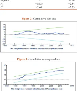
We also exploit both cumulative sum (CUSUM) and CUSUM squared (CUSUMQ)tests for structural stability. Figures 2 and 3 respectively show CUSUM of recursive residuals and CUSUMQ of recursive residuals considering a 95% confidence interval.
Table 1: Dynamic equation results
Variables Coefficient t-statistic
C −1.32 −4.16
logPCONt−1 0.50 6.18
logGDPt 0.56 6.22
Pt −0.002 −3.84
R2:0.99, DW: 1.93. GDP: Gross domestic product, PCON: Private consumption
Table 2: Estimation’s goodness of fit
Hypotheses P [LM Version]
Serial correlation 0.950 Functional form 0.958
Normality 0.415
Heteroskedasticity 0.316
Table 3: ECM
Variables Coefficient t-statistic
dlogGDPt 0.56 6.22
dPt −0.002 −3.84
dC −1.32 −4.16
ECM(−1) −0.49 −6.16
R2: 0.74, DW: 1.93. ECM: Error correction model, GDP: Gross domestic product
Table 4: Long-run relations
Variables Coefficient t-statistic
logGDPt 1.13 32.24
Pt −0.005 −2.84
C −2.64 −5.33
Figure 2: Cumulative sum test
According to Figures 2 and 3, as the curves didn’t intersect the straight lines, the hypothesis of structural stability is accepted.
5. CONCLUSION AND POLICY
IMPLICATIONS
Due to the importance of consumption in both demand side of an economy and also in economic policy-making, further studies in this area is in the dire need of attention. This study has shown that there is a positive and significant correlation between private consumption and GDP and also has considered the correlation between private consumption and inflation which is negative and significant. Other results can be noted that the consumption reaction to GDP in short-run is less than the long-run. Also, the effect of inflation on GDP in long-run is more than in short-run, which represents that consumers adjust their consumption in long-run, once they correct their expectations. Our suggestion respect to the large proportion of GDP which is dedicated to consumption, is that to consider the supply side policies in long-run along with enhancement in private consumption due to its effect on inflation declining and controlling, which would be useful and necessary for economic stability and progressing.
REFERENCES
Ahmad, M., Tashkini, A., Soori, A.R. (2008), Private consumption estimation in Iran economy. Journal of Economic Research, 8, 15-39 (In Persian).
Alpizar, F., Carlsson, F., Johansson-Stenman, O. (2005), How much do we care about absolute versus relative income and consumption? Journal of Economic Behavior & Organization, 56, 405-421. Ando, A., Modigliani, F. (1963), The life-cycle hypothesis of saving:
Aggregate implications and tests. American Economic Review, 53(1), 55-84.
Arabmazar, A., Noferesti, M. (2006), A macroeconometric model for Iran economy. Journal of Economic Trend, 20, 5-39 (In Persian). Baltagi, B.H. (2008), Econometrics. 4th ed. Heidelberg: Springer-Verlag.
p154, 155.
Banerjee, A., Dolado, J.J., Mestre, R. (1992), On some simple tests for
cointegration: The cost of simplicity. Discussion Paper No.7. Institute of Economics, Aarhus University, Aarhus.
Campbell, J.Y., Mankiw, N.G. (1989), Consumption, income, and interest rates: Reinterpreting the time series evidence. NBER Macroeconomics Annual, 4, 185-216.
CBI. (2014), Time Series Database. Central Bank of Iran. Available from: http://www.tsd.cbi.ir. [Last accessed on 2015 Feb 12].
Duesenberry, J.S. (1949), Income, Saving and the Theory of Consumer Behaviour. Cambridge: Harvard University Press.
Fakhrai, E., Mansouri, S.A. (2008), Estimation of long-run consumption function using ARDL approach and short-run consumption relation calculation of Iran. Journal of Quantitative Economics, 2, 23-48 (In Persian).
Fernandez-Villaverde, J., Krueger, D. (2011), Consumption and saving over the life cycle: How important are consumer durables? Macroeconomic Dynamics, 15, 725-770.
Friedman, M. (1957), A Theory of Consumption Function. Princeton: Princeton University Press.
Hall, R.E. (1987), Consumption. NBER Working Paper No. 2265. p1-30. Kwan, Y.K. (2006), The Direct Substitution between Government and
Private Consumption in East Asia. National Bureau of Economic Research (NBER), Working Paper No. 12431.
Mankiw, N.G. (2012), Macroeconomics. 8th ed. New York: Worth
Publishers. p465-467, p492.
Mankiw, N.G. (1982), Hall consumption hypothesis and durable goods. Journal of Monetary Economics, 10, 417-425.
Modigliani, F., Brumberg, R.H. (1954), Utility analysis and the consumption function: An interpretation of cross-section data. In: Kurihara, K.K., editor. Post Keynesian Economics. New Brunswick, NJ: Rutgers University Press. p388-436.
Romer, D. (2012), Advanced Macroeconomics. 4th ed. New York:
McGraw-Hill.
Soori, A. (2013), Applied Econometrics using Eviews 8 and Stata 12. Tehran: Farhangshenasi Publication (In Persian).
Tashkini, A. (2014), Applied Econometrics using Microfit. Tehran: Noor-e-Elm Publication. p140 (In Persian).
Valadkhani, A. (1997), Estimation and analysis of private consumption function in Iran (1959-1995) with integration approach. Journal of Planning and Budgeting, 16 and 17, 3-14 (In Persian).
Estimation results: (Microfit 4.1)