Using water–solvent systems to estimate in vivo blood–tissue partition coefficients

(1)

RESEARCH ARTICLE

Using water–solvent systems to estimate

in vivo blood–tissue partition coefficients

Caitlin E. Derricott

1

_{, Emily A. Knight}

1

_{, William E. Acree Jr.}

2

_{and Andrew SID Lang}

1*

Abstract

Background: Blood–tissue partition coefficients indicate how a chemical will distribute throughout the body and are an important part of any pharmacokinetic study. They can be used to assess potential toxicological effects from exposure to chemicals and the efficacy of potential novel drugs designed to target certain organs or the central nerv-ous system. In vivo measurement of blood–tissue partition coefficients is often complicated, time-consuming, and relatively expensive, so developing in vitro systems that approximate in vivo ones is desirable. We have determined such systems for tissues such as brain, muscle, liver, lung, kidney, heart, skin, and fat.

Results: Several good (p < 0.05) blood–tissue partition coefficient models were developed using a single water– solvent system. These include blood–brain, blood–lung, blood–heart, blood–fat, blood–skin, water–skin, and skin permeation. Many of these partition coefficients have multiple water–solvent systems that can be used as models. Several solvents—methylcyclohexane, 1,9-decadiene, and 2,2,2-trifluoroethanol—were common to multiple models and thus a single measurement can be used to estimate multiple blood–tissue partition coefficients. A few blood–tis-sue systems require a combination of two water–solvent partition coefficient measurements to model well (p < 0.01), namely: blood–muscle: chloroform and dibutyl ether, blood–liver: N-methyl-2-piperidone and ethanol/water (60:40) volume, and blood–kidney: DMSO and ethanol/water (20:80) volume.

Conclusion: In vivo blood–tissue partition coefficients can be easily estimated through water–solvent partition coef-ficient measurements.

Keywords: Blood–tissue partition coefficients, Abraham model, Blood–brain barrier, Pharmacokinetics

© 2015 Derricott et al. This article is distributed under the terms of the Creative Commons Attribution 4.0 International License (http://creativecommons.org/licenses/by/4.0/), which permits unrestricted use, distribution, and reproduction in any medium, provided you give appropriate credit to the original author(s) and the source, provide a link to the Creative Commons license, and indicate if changes were made. The Creative Commons Public Domain Dedication waiver (http://creativecommons.org/ publicdomain/zero/1.0/) applies to the data made available in this article, unless otherwise stated.

Background

When a chemical enters the body, either through absorp-tion or through direct administraabsorp-tion, the relative con-centrations found in the blood and other tissues are determined by physiochemical processes that separate the different parts of the body. For example, the blood– brain barrier separates the blood from the brain’s extra-cellular fluid in the central nervous system and protects the brain from potential neurotoxins and bacteria while allowing passage of essential molecules such as water, glucose, and amino acids that are crucial to neural function.

Knowing or predicting the partition coefficients (ratio of concentrations) of compounds between the blood-stream and various tissues is important in order to study the pharmacokinetic profile of drug candidates. While in vivo measurements are of most value, obtaining them is often not practical. Thus over the years several mod-els have been developed to predict blood–tissue partition coefficients [1–3], with recent special attention being paid to the blood–brain barrier [4, 5].

Linear free energy relationships, developed by Abra-ham [6], have been applied directly to blood–tissue parti-tion coefficients by Abraham, Gola, Ibrahim, Acree, and Liu [1] resulting in the model

where log BB is the base ten logarithm of the blood–brain partition coefficient; E, S, A, B, and V are the standard solute descriptors [7, 8] and c, e, s, a, b, v, and i are the

(1)

log BB=c+eE+sS+aA+bB+vV +il_c

Open Access

*Correspondence: alang@oru.edu

1_{Computing and Mathematics Department, Oral Roberts University,}

Tulsa, OK 74171, USA

(2)

process coefficients, see Table 1. The descriptor Ic is an

indicator variable for carboxylic acids that is taken to be one if the solute is a carboxylic acid and zero otherwise. This flag is not usually included in a general Abraham-type model but is needed here because the pH of blood is 7.4 and carboxylic acids are ionized at this pH.

Abraham and Acree have also used Eq. (1) to show that the water–1,9-decadiene system can be used as an excel-lent model for permeation through egg lecithin bilayers [9]. This suggests that other water–solvent systems could be used as models for blood–tissue coefficients. This would be very useful, because then in vivo blood–tissue partition coefficients could be estimated in vitro.

Methods

Abraham model coefficients have been determined for over 90 organic solvents and can be predicted for others [10]. To find water–solvent systems that could be used to approximate blood–tissue systems we regressed the e, s, a, b, and v coefficients for each of the 90 organic solvents against the e, s, a, b, and v coefficients for each blood–tis-sue system listed in Table 1 above. The c-coefficient was not included as it is the intercept and could be adjusted separately after the regression had been performed. Spe-cifically, we used linear regression in R (v 3.1.1)—‘lm’ command—and determined the best fit by using ‘regsub-sets’ command in the ‘leaps’ package.

For example, the logarithm of partition coefficient for the blood–brain barrier is:

Regressing Abraham solvent coefficients against this equation, we find that the water–methylcyclohexane par-tition system

(2)

log BB=0.547+0.221 E−0.604 S

−0.641 A−0.681B+0.635V−1.216 lc

(3)

log P_mcy=0.246+0.782 E−1.982S

−3.517 A−4.293B+4.528V

can be used as a good (p < 0.002, R2₌_{0.94) model for}

blood–brain barrier partition coefficients as follows:

where log Pmcy is the measured log P value for

methyl-cyclohexane. For additional details, datasets, and the R-code used, see the Open Notebook lab page [11].

Substituting Eq. (3) into (4) gives:

Comparing Eqs. (2) and (5) we see fairly good agree-ment between coefficients. To validate our model we plotted the predicted log BB values for water, for six inorganic gases and for 13 common organic compounds using both equations, see Table 2; Additional file 1: Appendix Table S1; Fig. 1.

The mean-square-error (MSE) between Eqs. (2) and (4) is 0.03 log units. The largest error occurs for styrene (AE 0.93 log units). In fact, without styrene, the MSE would drop to 0.02 log units. The reason why styrene is an out-lier is that it is on the edge on the training-set chemical space. It has E and S values of 0.85 and 0.65 respectively as compared to the average values of E and S for the other compounds in the training set of 0.16 and 0.24 respec-tively. Other solvents that could be used as model sys-tems for the blood–brain barrier include 1,9-decadience and octane.

We have modeled log BB indirectly by comparing the Abraham coefficients for water–solvent systems to the Abraham coefficients for log BB. We found that the water–methylcyclohexane system may be a good system to use to approximate log BB values in vitro, especially for solutes whose descriptor values fall within the range covered by both Abraham models (log BB and log Pmcy).

That is, Eq. (4) can be used to predict log BB values from log Pmcy values but should be used with caution when

(4)

log BB=0.505+0.169log P_mcy−1.216 Ic

(5)

log BB=0.547+0.132 E−0.335S

−0.594A−0.726 B+0.765 V−1.216 lc

Table 1 Coefficients in equation one for in vivo processes at 37 °C [1]

Process c e s a b v i

Blood–brain 0.547 0.221 −0.604 −0.641 −0.681 0.635 −1.216

Blood–muscle 0.082 −0.059 0.010 −0.248 0.028 0.110 −1.022

Blood–liver 0.292 0.000 −0.296 −0.334 0.181 0.337 −0.597

Blood–lung 0.269 0.000 −0.523 −0.723 0.000 0.720 −0.988

Blood–kidney 0.494 −0.067 −0.426 −0.367 0.232 0.410 −0.481

Blood–heart 0.132 −0.039 −0.394 −0.376 0.009 0.527 −0.572

Blood–fat 0.077 0.249 −0.215 −0.902 −1.523 1.234 −1.013

Blood–skin −0.105 −0.117 0.034 0.000 −0.681 0.756 −0.816

Water–skin 0.523 0.101 −0.076 −0.022 −1.951 1.652 0.000

(3)

using it with compounds outside the chemical space used to create these models. In addition, the MSE of 0.03 is between Eqs. (2) and (4) and we do not claim that Eq. (4) will have this type of performance when used to predict measured log BB values. Our work indicates that methyl-cyclohexane is a good candidate for approximating log BB values but future work should focus on modeling log

BB directly from log Pmcy when measured values for both

log BB and log Pmcy are known for a significant number

of compounds. Of particular interest would be experi-mentally determining both log BB and log Pmcy values for

more common organic compounds (including crystalline compounds) that span a larger range of solute descrip-tors. The 20 compounds that are common to both the log BB and log Pmcy databases are inorganic gases and liquid

organic compounds. The organic compounds, while not pharmaceutical compounds, are ones that workers are exposed to in chemical manufacturing processes.

Results and discussion

We have seen that methylcyclohexane can be used to approximate log BB using Eq. (4). In general, we approxi-mate the blood–tissue partition coefficient using the fol-lowing equation

where c0 is the intercept, c1 is the coefficient multiplier

for the log P system corresponding to solvent X1, and Ic is

the carboxylic acid flag. Performing a similar analysis as described above and regressing the water–solvent system Abraham coefficients against the blood–tissue systems given in Table 1, we find the following results, presented in tables, see Tables 3, 4, 5, 6, 7, 8, 9, 10, 11, 12, where the p-values are the standard p-values from linear regres-sion—calculated using the ‘lm’ command in R.

(6)

log P_blood/tissue=c0+c1X1+Ic Table 2 Predicted blood–brain barrier partition coefficients

Compound E S A B V log BB Eq. (2) log Pmcy log BB Eq. (4)

Water 0.00 0.45 0.82 0.35 0.167 −0.38 −4.01 −0.17

Ethanol 0.25 0.42 0.37 0.48 0.449 0.07 −1.78 0.20

1-Propanol 0.24 0.42 0.37 0.48 0.590 0.16 −1.05 0.33

Acetone 0.18 0.70 0.04 0.49 0.547 0.15 −0.90 0.35

t-Butanol 0.18 0.30 0.31 0.60 0.731 0.26 −0.56 0.41

2-Methyl-1-propanol 0.22 0.39 0.37 0.48 0.731 0.26 −0.41 0.44

1-Butanol 0.22 0.42 0.37 0.48 0.731 0.24 −0.40 0.44

Neon 0.00 0.00 0.00 0.00 0.085 0.60 0.60 0.61

Argon 0.00 0.00 0.00 0.00 0.190 0.67 1.02 0.68

Nitrogen 0.00 0.00 0.00 0.00 0.222 0.69 1.06 0.68

Krypton 0.00 0.00 0.00 0.00 0.246 0.70 1.25 0.72

Methane 0.00 0.00 0.00 0.00 0.250 0.71 1.34 0.73

Xenon 0.00 0.00 0.00 0.00 0.329 0.76 1.61 0.78

Sulphur Hexafluoride –0.60 –0.20 0.00 0.00 0.464 0.83 2.36 0.90

Benzene 0.61 0.52 0.00 0.14 0.716 0.73 2.38 0.91

Toluene 0.60 0.52 0.00 0.14 0.857 0.81 2.90 1.00

Ethylbenzene 0.61 0.51 0.00 0.15 0.998 0.91 3.44 1.09

Cyclohexane 0.31 0.10 0.00 0.00 0.845 1.09 4.07 1.19

Methylcyclohexane 0.24 0.06 0.00 0.00 0.986 1.19 4.75 1.31

Styrene 0.85 0.65 0.00 0.16 0.955 0.84 5.15 1.38

(4)

Examining the results presented in the Tables 3, 4, 5, 6, 7, 8, 9, 10, 11, 12, we see that the blood–brain barrier sys-tem can be modeled well with multiple solvents, includ-ing methylcyclohexane, octane, and 1,9-decadiene.

The results for blood–muscle and blood–liver were similar, with similar solvents, but very poor R2_values

overall. The highest R2_{was 0.44, exhibited by}

2,2,2-trif-luoroethanol for the blood–liver system.

The results for modeling the blood–lung, blood– kidney, and blood–heart partition coefficients were interesting as the top three suggested replacement sol-vents were identical, namely: 2,2,2-trifluoroethanol,

Table 3 Top five solvents for blood–brain

Solvent c0 c1 p R2

Methylcyclohexane 0.505 0.169 0.001 0.94

Octane 0.510 0.160 0.002 0.92

1,9-Decadiene 0.529 0.173 0.003 0.92

Cyclohexane 0.522 0.157 0.003 0.91

Decane 0.517 0.160 0.003 0.91

Table 4 Top five solvents for blood–muscle

Chloroform 0.077 0.028 0.2 0.41

2,2,2-Trifluoroethanol 0.063 0.047 0.2 0.38

Dichloromethane 0.074 0.025 0.2 0.35

Carbon tetrachloride 0.078 0.022 0.2 0.34

Iodobenzene 0.086 0.022 0.2 0.32

Table 5 Top five solvents for blood–liver

1,9-Decadiene 0.287 0.044 0.3 0.30

Chloroform 0.283 0.048 0.3 0.28

2,2,4-Trimethylpentane 0.279 0.040 0.3 0.27

Table 6 Top five solvents for blood–lung

1,9-Decadiene 0.256 0.124 0.07 0.60

Chloroform 0.243 0.135 0.08 0.58

Table 7 Top five solvents for blood–kidney

1,9-Decadiene 0.489 0.052 0.3 0.26

Chloroform 0.483 0.055 0.3 0.23

Table 8 Top five solvents for blood–heart

1,9-Decadiene 0.124 0.081 0.08 0.59

Octane 0.115 0.072 0.09 0.54

Table 9 Top five solvents for blood–skin

Ethanol/water(10:90)vol 0.192 1.716 0.0002 0.98 N,N-Dimethylformamide −0.058 0.153 0.0002 0.98 Ethanol/water(20:80)vol 0.099 0.811 0.0004 0.97 Ethanol/water(70:30)vol −0.120 0.234 0.0005 0.96 Ethanol/water(30:70)vol 0.034 0.517 0.0006 0.96

Table 10 Top five solvents for blood–fat

Carbon disulfide 0.065 0.256 0.000001 0.998

Ethylbenzene 0.049 0.297 0.00002 0.99

p-Xylene 0.028 0.297 0.00002 0.99

o-Xylene 0.052 0.298 0.00002 0.99

Peanut oil −0.128 0.358 0.0008 0.95

Table 11 Top five solvents for water–skin

THF 0.438 0.383 0.000003 0.997

Dibutylformamide 0.389 0.403 0.00002 0.99

1,4-Dioxane 0.474 0.401 0.00002 0.99

Acetone 0.395 0.410 0.00003 0.99

N-Formylmorphine 0.538 0.475 0.00003 0.99

Table 12 Top five solvents for skin-permeation

Methyl tert-butyl ether −5.588 0.492 0.00002 0.99

THF −5.532 0.501 0.0002 0.99

Diethyl ether −5.596 0.503 0.0004 0.99

(5)

methylcyclohexane, and 1,9-decdiene. The R2_{values for}

these systems ranged between 0.41 for blood–kidney to 0.72 for blood–heart.

The blood–skin barrier model showed very strong results, with all of the top 5 R2_{values above 0.95, which}

is very good. Some previously unseen solvents came up, the various ethanol–water mixtures composed four of the top five solvents.

Modeling the blood–fat system also had some very promising results. The highest was carbon disulfide with an R2_{of 0.998. The lowest of the top 5 values was still}

very good, an R2_{value of 0.95 for peanut oil. We suggest}

using the water/peanut oil system as a replacement sys-tem for blood–fat partition coefficients.

The water–skin solvents tested also produced strong results; the lowest of the top five R2_{values is over 0.9,}

much higher than several of the earlier systems. Tetrahy-drofuran resulted in the highest R2_{value at 0.997.}

The top five suggested replacement water–solvent sys-tems for skin-permeation, like many previous blood–tis-sue systems, show great promise. The top three solvents

being methyl tert-butyl ether, tetrahydrofuran, and die-thyl ether.

Whilst most blood–tissue systems can be modeled with a single water–solvent system, blood–muscle, blood– liver, and blood–kidney had poor results, with R2_values

all below 0.45. This is due to these three solvents having the smallest v values (0.110, 0.337, and 0.410) and high-est b values (0.028, 0.181, 0.232) taking them out of the chemical space for single solvents. For these systems we modeled the blood–tissue coefficients using two meas-ured water–solvent partition coefficient values X1 and X2

as follows

where again c0 is the intercept. The results of these

mod-els are again presented in table form, see Tables 13, 14, 15.

Blood–kidney regression with 1-variable produced very poor results, the top R2_{value was 0.4 for}

2,2,2-trifluoro-ethanol. Two variables can be used to increase the R2

value. This greatly improved all values for blood–kidney,

(7)

log P_blood/tissue=c0+c1X1+c2X2+Ic

Table 13 Top five results for two-variable blood–kidney partition coefficient

Solvent 1 Solvent 2 c0 c1 c2 p R2

Ethanol/water(20:80)vol DMSO 0.924 2.035 −0.428 0.0001 0.998

Ethanol/water(30:70)vol DMSO 0.754 1.268 −0.417 0.001 0.99

Ethanol/water (40:60)vol DMSO 0.617 0.916 −0.410 0.001 0.99

2-Butanol Tributyl phosphate 0.408 0.799 −0.698 0.002 0.99

Ethanol/water(20:80)vol Formamide 1.014 2.596 −0.786 0.03 0.90

Table 14 Top five results for two-variable blood–liver partition coefficient

Ethanol/water(60:40)vol N-Methyl-2-piperidone 0.336 0.609 −0.352 0.002 0.99

Ethanol/water(70:30)vol N-Ethylformamide 0.366 0.806 −0.566 0.01 0.94

Octadecanol N-Methylpyrrolidinone 0.362 0.307 −0.278 0.02 0.92

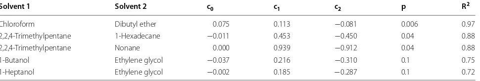
Table 15 Top five results for two-variable blood–muscle partition coefficient

Chloroform Dibutyl ether 0.075 0.113 −0.081 0.006 0.97

2,2,4-Trimethylpentane 1-Hexadecane −0.011 0.453 −0.450 0.04 0.88

2,2,4-Trimethylpentane Nonane 0.000 0.939 −0.912 0.04 0.88

1-Butanol Ethylene glycol −0.037 0.216 −0.310 0.1 0.75

(6)

the top value produced by a mixture of ethanol/water (20:80) and DMSO, with an R2_{value of 0.997.}

Blood–liver also produced very poor 1-variable results, so 2-variables were used to improve the R2_{value. The}

highest R2_{with 1-variable was 0.44 with}

2,2,2-trifluoro-ethanol. The highest R2_{with 2-variables was 0.99 by}

etha-nol/water (60:40) and N-methyl-2-piperidone.

For the blood–muscle process, the overall 2-variable correlation coefficients were fairly good. The solvents that are best are chloroform and dibutyl ether with an R2

value of 0.97.

Combining two measured water/solvent partition coef-ficients can also improve the models for approximation the other blood–tissue partition coefficient values. See the Wiki page in the references for a complete list of all two-variable data tables [11].

When looking at the results, we note that the stand-ard 1-octanol/water partition coefficient (log P) does not appear as a top solvent for any of the blood–tissue processes. This is interesting because log P has for a long time been assumed to be useful in estimating the distribution of drugs within the body and is a standard descriptor used in most QSAR modeling. Since the use of log P is prevalent throughout the chemistry community, we calculated how well the Abraham model for every blood–tissue partition coefficient can be modelled by the Abraham model for log P, see Table 16.

Examining Table 16, we see that log P can be used to approximate all blood–tissue partition coefficients and actually performs moderately well for estimating log BB, but poorly for blood–muscle and all other organs. How-ever, log P seems like a reasonable measure for processes to do with chemicals entering into the body: blood–skin, blood–fat, water–skin, and skin-permeation. The lat-ter observation is in accord with the published results of Cronin and coworkers [12, 13] who noted that the per-cutaneous adsorption of organic chemicals through skin

is mediated by both the hydrophobicity (log P) and the molecular size of the penetrant.

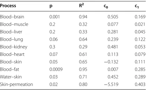
The water/solvent systems that included methylcy-clohexane and 1,9-decadiene were in the top 5 results for multiple regressions. In Tables 17 and 18 we present the Eq. (6) coefficients for methylcyclohexane and 1,9-deca-dience respectively. In some case the coefficients have low R2_{values. Keeping that in mind, we have a two more}

ways (with better performance than log P for predicting the important log BB partition coefficient) that all blood– tissue partition coefficients can be approximated by a sin-gle water–solvent partition coefficient measurement.

As we have seen, methylcyclohexane is a good solvent when used to model the blood–brain barrier process. For other processes, blood–fat and skin-permeation, it showed a reasonably good R2_{value (over 0.80). However,}

blood–muscle, blood–liver, and blood–kidney showed really poor R2_{values (all less than 0.33).}

1,9-Decadiene was just as good of a solvent as methyl-cyclohexane for approximating multiple blood–tissue coefficients. Blood–brain, blood–fat, and skin-permea-tion all showed good R2_{values over 0.80. Just as in the}

Table 16 Equation (6) coefficients for 1-octanol against multiple processes

Process p R2 _c

0 c1

Blood–brain 0.06 0.64 0.553 0.171

Blood–muscle 0.7 0.03 0.082 0.008

Blood–liver 0.6 0.07 0.293 0.026

Blood–lung 0.3 0.27 0.272 0.097

Blood–kidney 0.6 0.07 0.495 0.032

Blood–heart 0.3 0.31 0.134 0.070

Blood–skin 0.003 0.92 −0.100 0.161

Blood–fat 0.01 0.82 0.088 0.324

Water–skin 0.0003 0.97 0.537 0.415

Skin-permeation 0.0004 0.97 −5.402 0.545

Table 17 Equation (6) coefficients for methylcyclohexane against multiple processes

Process p R2 _c

0 c1

Blood–brain 0.001 0.94 0.505 0.169

Blood–muscle 0.2 0.32 0.077 0.021

Blood–liver 0.2 0.33 0.281 0.045

Blood–lung 0.06 0.64 0.239 0.122

Blood–kidney 0.3 0.29 0.481 0.053

Blood–heart 0.07 0.61 0.113 0.079

Blood–skin 0.05 0.65 −0.132 0.111

Blood–fat 0.0009 0.95 0.007 0.285

Water–skin 0.03 0.71 0.452 0.289

Skin-permeation 0.02 0.80 −5.519 0.403

Table 18 Equation (6) coefficients for 1,9-decadiene against multiple processes

Process p R2 _c

0 c1

Blood–brain 0.003 0.92 0.529 0.173

Blood–muscle 0.3 0.29 0.080 0.021

Blood–liver 0.3 0.30 0.287 0.044

Blood–lung 0.07 0.60 0.256 0.124

Blood–kidney 0.3 0.26 0.489 0.050

Blood–heart 0.08 0.59 0.124 0.080

Blood–skin 0.04 0.71 −0.117 0.120

Blood–fat 0.0005 0.96 0.046 0.297

Water–skin 0.02 0.76 0.491 0.311

(7)

methylcyclohexane case, the processes blood–mus-cle, blood–liver, blood–kidney were not well modeled and 2-solvent models are needed for more accurate approximations.

The research presented in this paper was performed under standard Open Notebook Science conditions, where day-to-day results were posted online in as near to real time as possible. For addition details, the data files, and the R-code used to find model systems, see the Open Lab Notebook page [11].

Conclusions

Replacement solvents for various blood–tissue processes are proposed based upon the Abraham general solvation linear free energy relationship (1). For example, the top five solvents for approximating the blood brain barrier partition coefficient are methylcyclohexane, 1,9-decadi-ene, octane, cyclohexane, and decane. The five best sol-vents for the other blood–tissue partition coefficients were also calculated and presented. For three systems: muscle, liver, and lung; two-solvent models were pre-sented to improve accuracy. For 1-solvent models, two solvents regularly came up in the list of best solvents for many processes. The top two recurring solvents were methylcyclohexane and 1,9-decadiene. This sug-gests that a single water–solvent partition measurement could in either methylcyclohexane or 1,9-decadiene can be used to approximate several blood–tissue partition coefficients.

Abbreviations

THF: tetrahydrofuran; DMSO: dimethyl sulfoxide; MSE: mean square error; BB: blood–brain; MCY: methylcyclohexane.

Authors’ contributions

CED and EAK performed all the modeling in this paper recording their results using Open Notebook Science and helped write the manuscript; ASIDL helped write the manuscript; WEA collected and curated the methylcyclohex-ane partition data and helped write the manuscript. All authors read and approved the final manuscript.

Author details

1_{Computing and Mathematics Department, Oral Roberts University, Tulsa, OK}

74171, USA. 2_{Department of Chemistry, University of North Texas, 1155 Union}

Cir, Denton, TX 76203, USA.

Acknowledgements

We dedicate this article to Dr. Jean-Claude Bradley who more than anyone espoused the value of Open Notebook Science in the scientific process. With-out him, this article would not have been possible.

Additional file

Additional file 1. Measured and predicted Log BB values for 20 organic compounds.

Competing interests

The authors declare that they have no competing interests.

Received: 28 May 2015 Accepted: 30 September 2015

References

1. Abraham MH, Gola JMR, Ibrahim A, Acree WE Jr, Liu X (2015) A simple method for estimating in vitro air-tissue and in vivo blood–tissue parti-tion coefficients. Chemosphere 120:188–191

2. DeJongh J, Verhaar HJM, Hermens JLM (1997) A quantitative property-property relationship (QPPR) approach to estimate in vitro tissue-blood partition coefficients of organic chemicals in rats and humans. Arch Toxicol 72(1):17–25

3. Poulin P, Kannan K (1995) An algorithm for predicting tissue: Blood parti-tion coefficients of organic chemicals from n-octanol: water partiparti-tion coefficient data. J Toxicol Environ Health Part A 46(1):117–129 4. Bujak R, Struck-Lewicka W, Kaliszan M, Kaliszan R, Markuszewski M (2015)

Blood–brain barrier permeability mechanisms in view of quantitative structure–activity relationships (QSAR). J Pharm Biomed Anal 108:29–37 5. Jouyban A, Soltani S (2012) Blood brain barrier permeation. In: Acree WE

Jr (ed) Toxicity and Drug Testing. Intech. Instrument Society of America, Pittsburgh

6. Abraham MH (1993) Scales of solute hydrogen-bonding: their construc-tion and applicaconstruc-tion to physicochemical and biochemical processes. Chem Soc Rev 22(2):73–83

7. Abraham MH, Ibrahim A, Zissimos AM (2004) The determination of sets of solute descriptors from chromatographic measurements. J Chromatogr A 1037:29–47

8. Abraham MH, McGowan (1987) The use of characteristic volumes to measure cavity terms in reversed phase liquid chromatograph. Chroma-tographia 23(4):243–246. doi:10.1007/BF02311772

9. Abraham MH, Acree WE Jr (2012) Linear free-energy relationships for water/hexadec-1-ene and water/deca-1, 9-diene partitions, and for per-meation through lipid bilayers; comparison of perper-meation systems. New J Chem 36(9):1798–1806

10. Bradley J-C, Abraham MH, Acree WE Jr, Lang ASID (2015) Predicting Abraham model solvent coefficients. Chem Cent J 9:12. doi:10.1186/ s13065-015-0085-4

11. Lang ASID, Acree WE Jr, Derricott CE, Knight EA (2015) Blood–tissue partition coefficients. Approximating blood–tissue partition coefficient measurements. Open lab notebook page. http://oruopennotebooksci-ence.wikispaces.com/Blood-tissue+partition+coefficients

12. Cronin MTD, Dearden JC, Moss GP, Murray-Dickson G (1999) Investiga-tion of the mechanism of flux across human skin in vitro by quantitative structure-permeability relationships. Eur J Pharm Sci 7(4):325–330 13. Moss GP, Dearden JC, Patel JC, Cronin MTD (2002) Quantitative

structure-permeability relationships (QSPRs) for percutaneous adsorption. Toxicol In Vitro 16(3):299–317

Open access provides opportunities to our colleagues in other parts of the globe, by allowing

anyone to view the content free of charge.

Publish with

Chemistry

Central and every

scientist can read your work free of charge

W. Jeffery Hurst, The Hershey Company. available free of charge to the entire scientific community peer reviewed and published immediately upon acceptance cited in PubMed and archived on PubMed Central yours you keep the copyright

Submit your manuscript here: