Synchronization of Nonlinear Continuous-time Systems by Sampled-data
Output Feedback Control
*Jian Zhang
School of Automation Engineering, University of Electronic Science and Technology of China, Chengdu, China
e-mail: [email protected]
http://dx.doi.org/10.5755/j01.itc.43.1.2450
Abstract. The paper is concerned with the synchronization problem of a general class of multi-input multi-output (MIMO) nonlinear continuous-time systems under sampled-data output feedback control. The main contributions of the present paper are twofold: (i) we provide a unified synthesis method and synchronization criteria for MIMO Lipschitz nonlinear continuous-time systems; (ii) we present a systematic computable framework based on the sum of squares (SOS) and linear matrix inequality (LMI) software tools for polynomial nonlinear systems. From the viewpoint of observer theory, we design an observer driven by sampled-data output for Lipschitz nonlinear continuous-time systems, when the output of the plant can be measured only at sampling instants. Furthermore, the presented method can ensure exponential convergence of the observer error, rather than practical convergence. Finally, an illustrative example is also given to demonstrate the effectiveness of the proposed approach.
Keywords: nonlinear systems; synchronization; sampled-data control; state observers.
*
This work was supported by National Science Foundation of China (Project No. 61004048)
1. Introduction
Synchronization is an universal and important concept for dynamical systems. Among a number of research results in this area, a master-slave structure is usually taken as a typical model. Given a particular dynamical system called the master, together with an identical system, the aim is to synchronize the complete or partial response of the slave system to the master system, by using a signal derived from the master system. From the viewpoint of control theory, the master-slave synchronization scheme can also be seen as a special case of the observer design problem [1], which provides a solution framework based on nonlinear observer theory. This kind of observer-based approach has extensively been investigated in a number of research works [2-3].
Nowadays, modern controllers are typically implemented digitally and this strongly motivates investigation of sampled-data systems. Recent advancements in digital technology have rendered remarkable merit to digital control systems exhibiting flexibility in implementation of complex control algorithms [4].
To the best of our knowledge, the problem of sampleddata synchronization for a general class of
nonlinear systems has not been investigated and still remains challenging, which motivates the present study. Most of existing results are based on continuous-time synchronization controllers, which require the output of master systems be measured in continuous-time, and so are not implemented by digital devices. In addition, the problem of sampled-data synchronization is related to the called continuous-discrete observer from control theory, which has been considered for nonlinear systems based on the hybrid control approach and high-gain technique in [58]. However, these results only deal with some special classes of nonlinear systems, and can not apply to more general classes of nonlinear systems, which restricts the use of the methods. They are also not applicable to the systems studied in this paper.
application and effectiveness of the proposed approach.
2. Problem statement and preliminaries
Given a sampling period 𝑇> 0, consider the follo-wing general master-slave type of coupled systems under sampled-data output feedback controller
ℳ
:
�
𝑦
𝑥̇
(
(
𝑡
𝑡
) =
) =
ℎ�𝑥
𝑓
(
𝑥
(
(
𝑡
𝑡
))
)
�
𝑆
:
�
𝑥�̇
(
𝑡
) =
𝑓�𝑥�
(
𝑡
)
�
+
𝑢
(
𝑡
)
𝑦�
(
𝑡
) =
ℎ�𝑥�
(
𝑡
)
�
𝒸:
𝑢(𝑡)=−𝐾�𝑦(𝑡𝑘)−𝑦�(𝑡𝑘)�,𝑡𝑘≤𝑡<𝑡𝑘+1, 𝑡𝑘=𝑘𝑇, 𝑘=0,1,2,⋯,
(1)
which consists consists of master system ℳ, slave system 𝑆 and sampled-data controller 𝒸 with 𝑓(0) =
0, ℎ(0) = 0, where ℳ and 𝑆 are identical nonlinear systems with state vectors 𝑥,𝑥� ∈ 𝑅𝑛, and outputs 𝑦,𝑦� ∈ 𝑅𝑚 respectively, the mappings 𝑓 and ℎ are
nonlinear functions. The synchronization scheme (1) aims at synchronizing the slave system 𝑆 to the master system ℳ by employing sampled-data output feedback controller 𝒸. Then, our objective is to find a sampled-data controller gain matrix 𝐾, such that the synchronization error 𝑒̃(𝑡) =𝑥(𝑡)− 𝑥�(𝑡) is exponentially convergent to zero.
Remark 1. In fact, the formulated synchronization problem above can also be viewed as a special case of the observer design problem for nonlinear systems under the condition that the output of the plant is available only at sampling instants, i.e. the slave system with sampled-data controller can be treated as an observer driven by sampled-data output for the master system. The original theory and design procedures for continuous-time full-order observers driven by data output or delayed sampled-data output have been presented for linear time-invariant systems in the references [12-13].
Remark 2. It should be noted that it is significantly different between nonlinear sampled-data observer and nonlinear continuous-time observer driven by sampled-data output, although they all use only sampled data of the output. As we have known, a sampled-data observer can be modeled as discrete-time systems and observers driven by sampled data is a typical class of hybrid systems. A general design framework of sampled-data observer for nonlinear systems has been recently proposed based on an approximate discrete-time model and emulation method in [14], where the Duffing system has been also used as an illustrative example to show how these methods could be used. However, the resulting designs only can guarantee practical convergence rather than exponential convergence of the observer error, which means that the observer error converges
to a neighborhood of zero, rather than converges to zero, see also the references [15-16].
In the following part of the paper, we will make the further assumptions.
A1. The functions 𝑓(𝑥):𝑅𝑛→ 𝑅𝑛 and ℎ(𝑥):𝑅𝑛→ 𝑅𝑚 are differentiable with respect to 𝑥.
A2. Define Θ as a convex hull of Ω, where 𝛺 ⊂ 𝑅𝑛 is an open and connect set, and assume that the functions 𝑓(𝑥), ℎ(𝑥) satisfy the following conditions for 𝑥 ∈ Θ
−∞<𝛼𝑖,𝑗≤𝜕𝑓𝑖𝜕𝑥𝑗≤𝛼𝑖,𝑗<+∞,1≤𝑖,𝑗≤𝑛
−∞<𝛽𝑟,𝑠≤𝜕ℎ𝑟𝜕𝑥𝑠≤𝛽𝑟,𝑠<+∞,1≤𝑟≤𝑚,1≤𝑠≤𝑛,
(2)
where 𝛼𝑖,𝑗 and 𝛼𝑖,𝑗 are the lower and the upper bounds of elements of the Jacobian matrix of 𝑓(x) in Θ, respectively, 𝛽𝑟,𝑠 and 𝛽𝑟,𝑠 are the lower and the upper bounds of elements of the Jacobian matrix of ℎ(𝑥) in Θ.
Under the assumptions, the parameter vectors 𝜕𝑓𝑖
𝜕𝑥
evolve in a hyper-rectangle called the parameter box 𝒱ℋ𝑓⊂ 𝑅𝑛
2
with 2𝑛2 vertices defined by
ℋ𝑓=�𝛼=�𝛼1,1,⋯ 𝛼𝑖,𝑗,⋯,𝛼𝑛,𝑛��𝛼𝑖,𝑗∈ �𝛼𝑖,𝑗,𝛼𝑖,𝑗��. (3)
Similarly, the other parameter vectors 𝜕ℎ𝑟
𝜕𝑥 belong
to the hyper-rectangle 𝒱ℋℎ ⊂ 𝑅𝑛⋅𝑚 defined by the following set of 2𝑛⋅𝑚 vertices
ℋℎ=�𝛽=�𝛽1,1,⋯ 𝛽𝑟,𝑠,⋯,𝛽𝑚,𝑛��𝛽𝑟,𝑠∈ �𝛽𝑟,𝑠,𝛽𝑟,𝑠��. (4)
The assumptions imply that the differentiable functions 𝑓(𝑥), ℎ(𝑥) are locally Lipschitz continuous with Lips- chitz constants
𝛾𝑓=�� max(𝛼2𝑖,𝑗,𝛼𝑖2,𝑗) 𝑛,𝑛
𝑖,𝑗 ,𝛾ℎ =
�� max(𝛽𝑟2,𝑠,𝛽𝑟,𝑠 2
)
𝑚,𝑛
𝑟,𝑠 . (5)
It should be noted that the class of systems satisfying the assumptions includes a large variety of systems already studied in the past literatures, namely the class of differentiable Lipschitz nonlinear systems.
Lemma 1. Let 𝑔:𝑅𝑛→ 𝑅𝑝 and 𝑎,𝑏 ∈ 𝑅𝑛 . We assume that 𝑔 is differential on 𝐶𝐶(𝑎,𝑏). Then, there are constant vectors 𝑐1,⋯, 𝑐𝑞,⋯, 𝑐𝑝∈ 𝐶𝐶(𝑎,𝑏), 𝑐𝑞≠ 𝑎, 𝑐𝑞≠ 𝑏 for
𝑞= 1,⋯,𝑝, such that
𝑔(𝑎)− 𝑔(𝑏) =�� 𝑙𝑝𝑇(𝑞)𝑙𝑛(𝑖)𝜕𝑔𝜕𝑥𝑞𝑖(𝑐𝑖) 𝑝,𝑛
𝑞,𝑖=1 �(𝑎 − 𝑏), (6)
where 𝐶𝐶(𝑎,𝑏) = {𝜛𝑎+ (1− 𝜛)𝑏, 0 <𝜛< 1} is the convex combination of 𝑎 and 𝑏 , 𝑙𝑝(𝑞) =�0⋯0 𝑞𝑡ℎ1 0⋯0� ∈ 𝑅𝑝 , and 𝑙𝑛(𝑖) =
[0⋯0 𝑞𝑡ℎ1 0⋯0]∈ 𝑅𝑛 are the canonical bases of
the vectorial space 𝑅𝑝 and 𝑅𝑛 respectively.
Note that the lemma 1 provides an alternative to the usual Lipschitz property, which is directly used in most of the literatures. The reformulation can obviously lead to less restrictive results than the Lipschitz condition.
3. Main results
Theorem 1. Let us denote the index (𝑖,𝑗,𝑟,𝑠) as ℓ , where 1 <𝑖,𝑗,𝑠<𝑛 , 1 <𝑟<𝑚 . Given a sampling period 𝑇> 0, a constant 𝜆> 0, and a scalar 𝜀> 0, if there exist matrices 𝑃=𝑃𝑇 > 0, 𝑄=𝑄𝑇>
0 , 𝑅=𝑅𝑇 > 0, 𝑊ℓ=�𝑊ℓ
11 𝑊
ℓ12
∗ 𝑊ℓ22� ≥0
, and any
matrices 𝑁ℓ=�𝑁ℓ
1
𝑁ℓ2�
, 𝑀ℓ=�𝑀ℓ
1
𝑀ℓ2�
with appropriate
dimensions such that the following matrix inequalities hold for any 𝛼 ∈ ℋ𝑓 and𝛽 ∈ ℋℎ
Ξℓ1=
⎣ ⎢ ⎢ ⎡Φℓ11(𝛼)
∗ ∗ ∗
Φℓ12(𝛽)
Φℓ22
∗ ∗
−𝑀ℓ1
−𝑀ℓ2
−𝑒−𝜆𝑇𝑄
∗
𝜀𝑇𝐹𝑇(𝛼)𝑃
𝜀𝑇𝐻𝑇(𝛽)𝑅𝑇
0 −𝜀𝑃 ⎦⎥
⎥ ⎤
Ξℓ2=�𝑊∗ℓ 𝜀𝑒N−𝜆𝑇ℓ 𝑃� ≥0,1≤ ℓ ≤2𝑛
2+𝑛𝑚
Ξℓ3=�𝑊∗ℓ 𝜀𝑒M−𝜆𝑇ℓ 𝑃� ≥0,1≤ ℓ ≤2𝑛
2+𝑛𝑚
,
(7)
where
Φℓ11(𝛼) =𝑃𝐹(𝛼) +𝐹𝑇(𝛼)𝑃+𝜆𝑃+ (𝑁ℓ1)𝑇+
(𝑁ℓ1) +𝑄+𝑇𝑊ℓ11
Φℓ12(𝛽) =𝑅𝐻(𝛽) + (𝑁ℓ2)𝑇− 𝑁ℓ1+𝑀ℓ1+𝑇𝑊ℓ12
Φℓ22=−𝑁ℓ2−(𝑁ℓ2)T+𝑀ℓ2+ (𝑀ℓ2)𝑇+𝑇𝑊ℓ22, (8)
and
𝐹(𝛼) =�𝑛𝑖,𝑗=1,𝑛 𝑙𝑛𝑇(𝑖)𝑙𝑛(𝑗)𝜕𝑥𝜕𝑓𝑖 𝑗(𝛼)
𝐻(𝛽) =�𝑚𝑟,𝑠=1,𝑛 𝑙𝑚𝑇 (𝑟)𝑙𝑛(𝑠)𝜕ℎ𝜕𝑥𝑟𝑠(𝛽),
(9)
then, the synchronization error 𝑒̃(𝑡) is exponentially convergent to zero, and the sampled-data output feedback controller gain is given by 𝐾=𝑃−1𝑅.
▼Proof. From (1), the synchronization error dynamics can be represented as follows
𝑒̃̇(𝑡) =𝑓�𝑥(𝑡)� − 𝑓�𝑥�(𝑡)�+𝐾(𝑦(𝑡𝑘)− 𝑦�(𝑡𝑘)). (10)
By applying Lemma 1, it follows that
𝑒̃̇(𝑡) =𝐹�𝜃(𝑡)�𝑒̃(𝑡) +𝐾𝐻�𝜗(𝑡)�𝑒̃(𝑡𝑘), (11)
where
𝐹�𝜃(𝑡)�=�𝑛𝑖,𝑗=1,𝑛 𝑙𝑛𝑇(𝑖)𝑙𝑛(𝑗)𝜕𝑥𝜕𝑓𝑗𝑖(𝜃𝑖(𝑡))
𝐻�𝜗(𝑡)�=�𝑚𝑟,𝑠=1,𝑛 𝑙𝑚𝑇 (𝑟)𝑙𝑛(𝑠)𝜕ℎ𝜕𝑥𝑟𝑠(𝜗𝑟(𝑡))
(12)
and
𝜃𝑖(𝑡)∈{𝜅𝑓𝑥(𝑡) +�1− 𝜅𝑓�𝑥�(𝑡),𝜅𝑓∈[0,1]}
𝜗𝑟(𝑡)∈{𝜅ℎ𝑥(𝑡) + (1− 𝜅ℎ)𝑥�(𝑡),𝜅ℎ∈[0,1]}
𝜃(𝑡) =�𝜃1(𝑡),⋯,𝜃𝑛(𝑡)�,
𝜗(𝑡) =�𝜗1(𝑡),⋯,𝜗𝑚(𝑡)�.
(13)
Next, we represent the sampling instant 𝑡𝑘 as
𝑡𝑘 =𝑡 −(𝑡 − 𝑡𝑘) =𝑡 − 𝑑(𝑡), (14)
where 𝑑(𝑡) =𝑡 − 𝑡𝑘. It is obvious that 𝑑(𝑡) is a non-differentiable time-varying delay with bound 𝑇. As a result, the sampled-data output feedback controller 𝒸 in (1) can be written as a continuous-time controller with a time-varying piecewise-continuous delay 𝑢(𝑡) =−𝐾𝐻�𝜗(𝑡)�𝑒̃�𝑡 − 𝑑(𝑡)�. Then, it allows us to represent the error dynamics (10) as
𝑒̃̇(𝑡) =𝐹�𝜃(𝑡)�𝑒̃(𝑡) +𝐾𝐻�𝜗(𝑡)�𝑒̃(𝑡 − 𝑑(𝑡)).(15)
Choose a piecewise Lyapunov-Krasovskii functional to be
𝑉(𝑡) =𝑒̃𝑇(𝑡)𝑃𝑒̃(𝑡) +∫ 𝑒̃𝑡 𝑇(𝛿)𝑒𝜆(𝛿−𝑡)𝑄𝑒̃(𝛿)𝑑𝛿
𝑡−𝑇 +
∫ ∫ 𝜀𝑒̃̇𝑡 𝑇 𝑡+𝜏 0
−𝑇 (𝑣)𝑒𝜆(𝑣−𝑡)𝑃𝑒̃̇(𝑣)𝑑𝑣𝑑𝑑, (16)
which is positive definite, since 𝑃 and 𝑄 are positive definite matrices.
From the Leibniz-Newton formula, we have
2𝜉𝑇𝑁
ℓ�𝑒̃(𝑡)− 𝑒̃�𝑡 − 𝑑(𝑡)� − ∫𝑡−𝑑𝑡 (𝑡)𝑒̃̇(𝜂)𝑑𝜂�= 0
2𝜉𝑇𝑀
ℓ�𝑒̃�𝑡 − 𝑑(𝑡)� − 𝑒̃(𝑡 − 𝑇)− ∫𝑡−𝑇𝑡−𝑑(𝑡)𝑒̃̇(𝜂)𝑑𝜂�= 0,
(17)
In addition, for any matrix Wℓ=�Wℓ
11 W
ℓ12
∗ Wℓ22� ≥0
,
the following equation is also true
𝑇𝜉𝑇(𝑡)𝑊
ℓ𝜉(𝑡)− ∫𝑡−𝑑𝑡 (𝑡)𝜉𝑇𝑊ℓ𝜉(𝑡)𝑑𝑑−
∫ 𝜉𝑇𝑊
ℓ𝜉(𝑡)𝑑𝑑 𝑡−𝑑(𝑡)
𝑡−𝑇 = 0. (18)
When 𝑡 ∈[𝑡𝑘,𝑡𝑘+1) , differentiating (16) along trajectory of (15) and adding (17) and (18), it follows that
𝑉̇(𝑡) +𝜆𝑉(𝑡)≤ 𝜁𝑇Ξ�
ℓ
1𝜁 − ∫𝑡 𝜍𝑇
𝑡−𝑑(𝑡) (𝜂)Ξℓ2𝜍(𝜂)𝑑𝜂 −
∫𝑡−𝑑(𝑡)𝜍𝑇
𝑡−𝑇 (𝜂)Ξℓ3𝜍(𝜂)𝑑𝜂 (19)
holds, where
Ξ�ℓ1=�
Λ11 Λ12 −𝑀ℓ1
∗ Λ22 −𝑀ℓ2
∗ ∗ −𝑒−𝜆𝑇𝑄�
(20)
and
Λ11=Φℓ11�𝜃(𝑡)�+𝑇𝐹𝑇�𝜃(𝑡)�𝑃𝐹(𝜃(𝑡))
Λ12=Φℓ12�𝜗(𝑡)�+𝜀𝑇𝐹𝑇�𝜃(𝑡)�𝑃𝐾𝐻(𝜗(𝑡))
Λ22=Φℓ22+𝜀𝑇𝐻𝑇�𝜗(𝑡)�𝐾𝑇𝑃𝐾𝐻�𝜗(𝑡)�.
(21)
Denoting 𝑃𝐾=𝑅 , then, by using Schur complements, Ξ�ℓ1 is equivalent to
Ξ�ℓ1=
⎣ ⎢ ⎢
⎡Φℓ11(𝜃(𝑡))
∗ ∗ ∗
Φℓ12(𝜗(𝑡))
Φℓ22
∗ ∗
−𝑀ℓ1
−𝑀ℓ1
−𝑒−𝜆𝑇𝑄
∗
𝜀𝑇𝐹𝑇(𝜃(𝑡))𝑃
𝜀𝑇𝐻𝑇(𝜗(𝑡))𝑅𝑇 0
−𝜀𝑃 ⎦⎥ ⎥ ⎤
. (22)
When 𝑡 ∈[𝑡𝑘,𝑡𝑘+1), integrating (19) from 𝑡𝑘 to 𝑡 gives
𝑉(𝑡)≤ 𝑒−𝜆(𝑡−𝑡𝑘)𝑉(𝑡𝑘), (23)
which leads to
𝑉(𝑡)≤ 𝑒−𝜆𝑡𝑉(𝑡
0). (24)
In view of (16) again, it holds that
𝜆min(𝑃)‖𝑒̃(𝑡)‖2≤ 𝑉(𝑡), 𝑉(𝑡0)≤ ℏ‖𝑒̃(𝑡0)‖𝑐2, (25)
where
ℏ=𝜆max(𝑃) +𝑇𝜆max(𝑄) +𝜀𝑇 2
2 𝜆max(𝑃)
‖𝑒̃(𝑡)‖𝑐= sup0≤𝜙≤𝑇(𝑒̃(𝑡+𝜙),𝑒̃̇(𝑡+𝜙). (26)
Therefore, combining (23)-(25) yields
‖𝑒̃(𝑡)‖2≤ 𝑉(𝑡) 𝜆min(𝑃)≤
𝜆 𝜆min(𝑃)𝑒
−𝜆(𝑡−𝑡0)‖𝑒̃(𝑡0)‖𝑐2, (27)
which means that the error dynamics is exponentially convergent to zero.
As previously stated, the time-varying parameters 𝜃𝑖(𝑡) and 𝜗𝑟(𝑡) belong to the parameter boxes 𝒱ℋ𝑓
and 𝒱ℋℎ respectively. On the other hand, the parameter-dependent matrices given in (22) are affinely dependent on the elements 𝜃𝑖(𝑡) and 𝜗𝑟(𝑡). Then, it follows that 𝑉̇+𝜆𝑉 in (19) attains its maximum value at one or more vertices of 𝒱ℋ
𝑓 and
𝒱ℋℎ. Thus, if the inequalities in (7) are satisfied,
𝑉̇+𝜆𝑉 is negative and the theorem follows.▲
Remark 3. The constant scalar 𝜀 in (7) can be viewed as a tuning parameter. When solving the LMIs (7), one can search for a feasible solution by setting the value of 𝜀 in advance. The parameter 𝜀 can also be searched by the following algorithm. That is, setting an initial value of 𝜀 and solving Eq.(7), if there is a feasible solution, then stops. Otherwise, reducing it by half and solving Eq.(7) again until 𝜀 is smaller than some pre-specified threshold. If there is no feasible solution to the LMIs (7), the desired controller cannot be obtained via Theorem 1. However, it should be noted that there might still exist some controllers that can exponentially synchronize the master and slave systems since the result in Theorem 1 is only a sufficient condition.
Remark 4. 𝐹�𝜃(𝑡)� can be further represented by 𝐴+𝐹1�𝜃(𝑡)�, where 𝐴 is a constant matrix and
𝐹1�𝜃(𝑡)� is a parameter varying matrix. Denote
𝜌 �𝐹1�𝜃(𝑡)�� as the amount of nonzero elements in
𝐹1�𝜃(𝑡)�. Similarly, let 𝐻�𝜗(𝑡)�=𝐶+𝐻1�𝜗(𝑡)�,
where 𝐶 is also a constant matrix, and 𝜌 �𝐻1�𝜗(𝑡)�� is
defined as the amount of nonzero elements in 𝐻1�𝜗(𝑡)�. Then, for finding a sampled-data controller,
it is necessary to solve 2𝜌�𝐹1�𝜃(𝑡)��+𝜌�𝐻1�𝜗(𝑡)�� sets of LMIs, each set consisting of three LMIs in the form of (7). The proposed method may require a relatively large computation amount, if the value of 𝜌 �𝐹1�𝜃(𝑡)��+𝜌 �𝐻1�𝜗(𝑡)�� is high. However, the
controller gain computed by our approach depends on the bounds of 𝛼𝑖,𝑗 and 𝛽𝑟,𝑠, which can provide a less conservative result than using a Lipschitz constant of the system and avoid a high gain 𝐾.
determined using the customized function f i n d b o u n d provided by SOSTOOLS V2.0 [17] for multivariate polynomial nonlinear systems, i.e. 𝑓𝑖(𝑥) and ℎ𝑟(𝑥) are polynomial functions. In the case of
polynomial nonlinear systems, the bounds of 𝜕𝑓𝑖
𝜕𝑥𝑗 and 𝜕ℎ𝑟
𝜕𝑥𝑠 in Θ can be formulated as a standard constrained
opti¬mization problem of the following forms
𝑚𝑖𝑛.�𝜕𝑓𝑖
𝜕𝑥𝑗�,𝑎𝑛𝑑𝑚𝑖𝑛.� 𝜕ℎ𝑟 𝜕𝑥𝑠�
𝑠.𝑡.𝜓𝜄(𝑥)≥0,𝜄= 1,⋯,Γ,
(28)
and
𝑚𝑖𝑛.�−𝜕𝑓𝑖
𝜕𝑥𝑗�,𝑎𝑛𝑑𝑚𝑖𝑛.�− 𝜕ℎ𝑟 𝜕𝑥𝑠�
𝑠.𝑡.𝜓𝜄(𝑥)≥0,𝜄= 1,⋯,Γ,
(29)
which can be directly computed using the function f i n d b o u n d. Clearly, the technique allows the following estimation of bounds
𝛼𝑖,𝑗𝑚𝑖𝑛.�𝜕𝑓𝜕𝑥𝑖𝑗�,𝛼𝑖,𝑗=−𝑚𝑖𝑛.�−𝜕𝑓𝜕𝑥𝑖𝑗�,
𝛽𝑟,𝑠𝑚𝑖𝑛.�𝜕ℎ𝜕𝑥𝑟𝑠�,𝛽𝑟,𝑠=−𝑚𝑖𝑛.�−𝜕ℎ𝜕𝑥𝑟𝑠�.
(30)
Furthermore, the previous analysis can be summarized by the following design procedure for polynomial nonlinear systems.
Algorithm 1. Given a sampling period 𝑇> 0 and the polynomial nonlinear systems in (1), which are defined on a convex subset of the domain {𝑥|𝜓𝜄(𝑥)≥
0,𝜄= 1,⋯,Γ}.
Step 1. Select a convergence rate 𝜆 of synchroniza-tion error.
Step 2. Compute derivatives of the functions 𝑓𝑖(𝑥) and ℎ𝑟(𝑥).
Step 3. Solve the optimization program formulated in (28) and (29) using SOSTOOLS.
Step 4. Choose a value of the parameter 𝜀, and solve the LMI problem in (7). If the set of LMIs are feasible, then the controller gain is calculated and the sampled-data output feedback controller 𝒸 is obtained. Otherwise, reset the parameter 𝜀 and resolve the LMIs (7).
4. Example
Example. The following example called Duffing equation is borrowed from [18], which is illustrated by
ℳ:� 𝑥̇1
(𝑡) =𝑥2(𝑡)
𝑥̇2(𝑡) =𝑥1(𝑡)− 𝑥13(𝑡)
𝑦(𝑡) =𝑥1(𝑡) + 0.5𝑥2(𝑡).
(31)
As stated in the reference [18], it has three equilibrium points 𝑥1= (0, 0) , 𝑥2= (1, 0) , 𝑥3= (−1, 0). A compact positively invariant region
enclosing three typical trajectories for different initial states is contained within the region Θ=
{(𝑥1,𝑥2)||𝑥1|≤2, |𝑥2| < 1}.
Assume that the output of the plant is available only at sampling instants 𝑘𝑇, 𝑘= 0, 1, 2,⋯ , and 𝑇= 0.25𝑠, which means that the output signal is sampled 4 times per second. Let us choose the parameters to be 𝜀= 2 and 𝜆= 0.2. Applying our approach, we get the slave system driven by sampled-data output of the master system
𝑆:� 𝑥�̇1(𝑡) =𝑥�2(𝑡) + 1.3993⋅ �𝑦(𝑡𝑘)− 𝑦�(𝑡𝑘)� 𝑥�̇2(𝑡) =𝑥�1(𝑡) +𝑥�13(𝑡) + 6.6295⋅ �𝑦(𝑡𝑘)− 𝑦�(𝑡𝑘)�.
(32)
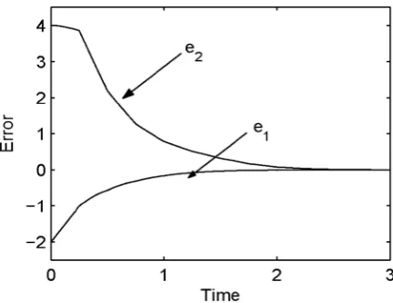
The simulation result in Fig. 1 shows the dynamics of synchronization errors 𝑒̃1(𝑡) =𝑥1(𝑡)—𝑥�1(𝑡) and 𝑒̃2(𝑡) =𝑥2(𝑡)—𝑥�2(𝑡) from two different initial
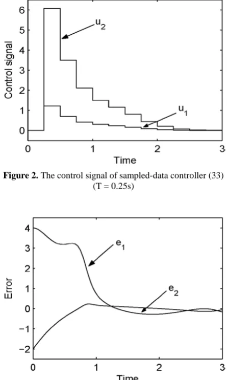
conditions 𝑥(0) = [−1 2]𝑇 and 𝑥�(0) = [1 −2]𝑇. The sampled-data control inputs
𝒸:�𝑢𝑢1(𝑡) = 1.3993⋅(𝑦(𝑡𝑘)− 𝑦�(𝑡𝑘))
2(𝑡) = 6.6295⋅(𝑦(𝑡𝑘)− 𝑦�(𝑡𝑘)) (33)
are also shown in Fig. 2, which remain constant over every sampling period. It can be observed that the re-sulting control performance is satisfactory.
Figure 1. The synchronization errors under the sampled-data controller (33)
Krener and Kang presented a method for designing continuous-time synchronization controllers for a class of single-input single-output (SISO) nonlinear systems with the triangular structure based on the
backstepping method, by which the continuous-time synchronization controller can be constructed as follows
𝒸:
⎩ ⎪ ⎨ ⎪
⎧ 𝑢1(𝑡)=−�𝑦(𝑡)−𝑦�(𝑡)� 3�1+𝑥�12(𝑡)�
3�−2−14𝑥�12(𝑡)−14𝑥�14(𝑡)−8𝑥�1(𝑡)𝑥�2(𝑡)−8𝑥�13(𝑡)𝑥�2(𝑡)−4𝑥�22(𝑡)+ 12𝑥�12(𝑡)𝑥�22(𝑡)−2𝑥�16(𝑡)�
𝑢2(𝑡)= �𝑦(𝑡)−𝑦�(𝑡)� 3�1+𝑥�12(𝑡)�
3�8 + 8𝑥�12(𝑡)+ 8𝑥�14(𝑡)−4𝑥�1(𝑡)𝑥�2(𝑡)+ 8𝑥�31(𝑡)𝑥�2(𝑡)+ 8𝑥�16(𝑡)+ 12𝑥�15(𝑡)𝑥�2(𝑡)−8𝑥�22(𝑡)24𝑥�12(𝑡)𝑥�22(𝑡)�
.(34)
Unlike the sampled-data controller (33), all component signals in the controller (34) must be measured in continuous-time. Consequently, the numerical simulations are carried out with the same initial conditions 𝑥�(0) = [1 −2]𝑇 as the previous slave system. Comparing Fig. 1 with Fig. 3 shows that the proposed method achieves a better performance.
Figure 2. The control signal of sampled-data controller (33) (T = 0.25s)
Figure 3. The synchronization errors under the continuous-time controller (34)
5. Conclusion
In this note, the problem of sampled-data synchronization has been studied for Lipschitz nonlinear continuous-time systems. A synchronization
criterion formulated in terms of LMIs has been derived to ensure the exponential stability of the resulting error dynamics under sampleddata output feedback control. A simulation example has been provided to illustrate the effectiveness of the developed approach.
References
[1] H. Nijmeijer, I. M. Y. Mareels. An observer looks at synchronization. IEEE Trans. Circuits Syst. I: Fundamental Theory and Applications, 1997, Vol. 44, 882−890.
[2] H. J. C. Huijberts, H. Nijmeijer, A. Pogromsky. Discrete-time observers and synchronization. In:
Guanrong Chen (eds.), Controlling Chaos and Bifurcations in Engineering Systems, CRC Press, 1999, 439−456.
[3] H. Nijmeijer. A dynamical control view on synchronization, Physica D - Nonlinear Phenomena, Vol. 154, pp. 219−228, 2001.
[4] D. S. Laila, D. Nešić, A. Astolfi. Sampled-data Control of Nonlinear Systems. In: Advanced Topics in Control Systems Theory II, Lecture notes from FAP 2005, Springer-Verlag, London, 2006, 91−137.
[5] V. Anderieu, M. Nadri. Observer design for Lipschitz systems with discrete-time measurements. In: Proc. 49th IEEE Conf. Decision Control, 2010, pp. 6522−6527.
[6] T. Raff, M. Kögel, F. Allgöwer. Observer with sample- and-hold updating for Lipschitz nonlinear systems with nonuniformly sampled measurements. In:
Proc. Amer. Contr. Conf., 2008, pp. 5254−5257.
[7] H. Hammouri, M. Nadri, R. Mota. Constant gain observer for continuous-discrete time uniformly observable systems. In: Proc. 45th IEEE Conf. Decision Control, 2006, pp. 5406−5411.
[8] T. Ahmed-Ali, R. Postoyan, F. Lamnabhi-Lagarrigue. Continuous-discrete Adaptive Observers for State Affine Systems. Automatica, 2009, Vol. 45, No. 12.
[9] E. Fridman, A. Seuret, J. P. Richard. Robust sampled−data stabilization of linear systems: an input delay approach. Automatica, 2004, Vol. 40, No. 8, 1441−1446.
[10] A. Zemouche, M. Boutayeb, G. Iulia Bara. Observer Design for Nonlinear Systems: An Approach Based on the Differential Mean Value Theorem. In: Proc. 44th Conf. Decision Control, 2005, pp. 6353−6358.
[12] G. H. Hostetter. Sampled data updating of continuous-time observers. IEEE Trans. Automat. Contr., 1976, Vol. 21, 272−273.
[13] A. Salama, V. Gourishankar. Continuous-time observers with delayed sampled data. IEEE Trans. Automat. Contr., 1978, Vol. 23, 1107−1109.
[14] M. Arcak, D. Nešić. A framework of nonlinear sampled−data observer design via approximate discrete-time models and emulation. Automatica, 2004, Vol. 40, 1931−1938.
[15] M. Abbaszadeh, H. J. Marquez. Robust Hobserver design for sampled-data Lipschitz nonlinear systems
with exact and Euler approximate models. Automatica, 2008, Vol. 44, 799−806.
[16] D. Nešić, A. R. Teel. Perspectives in robust control, ch.14. In: Sampled-data control of nonlinear systems: an overview of recent results. New York: Springer−Verlag. 2001.
[17] S. Prajna, A. Papachristodoulou, P. Seiler, P. A. Parrilo. SOSTOOLS and its control applications. Positive Polynomials in Control, 2005, Springer−Verlag, pp. 273−292.
[18] A. J. Krener, W. Kang. Locally convergent nonlinear observers. SIAM J. Contr. Optim., 2003, Vol. 42, 155−177.