1RQOLQHDU6\VWHP,GHQWLILFDWLRQLQ)UHTXHQWDQG,QIUHTXHQW
2SHUDWLQJ3RLQWVIRU1RQOLQHDU0RGHO3UHGLFWLYH&RQWURO
$OLUH]D)DWHKL
%HKQDQHK6DGHJKSRXU
%DWRRO/DELEL
1,2,3Advanced Process Automation & Control (APAC) research group,
Industrial Control Center of Excellence, Faculty of Electrical & Computer Engineering, K.N. Toosi University of Technology, Seyyed-Khandan, P.O.Box: 16315-1355, Tehran, Iran
e-mail: [email protected], [email protected]2, [email protected]3
http://dx.doi.org/10.5755/j01.itc.42.1.997
$EVWUDFW. This paper studies identification of a process in both frequent and infrequent operating points to design a nonlinear model predictive controller. Although, many of industrial processes normally work around an operating point, however they should seldom work in some infrequent points as well. In this case, due to low ratio of data points, identification of the processes based on all data set results in poor identification of the infrequent operating points. To resolve this problem, in this paper, at the first step, a data clustering strategy is used to group the data in different operating points. Since the ratio of infrequent to frequent data points is extremely low, the strategy used is the fuzzy Gath-Geva clustering methodology. Then, at the second step, a new approach has been proposed to compromise performance of identification of the nonlinear model for frequent and infrequent operating points. It is shown that if the ratio of data associated with frequent operating point to data of infrequent operating point is appropriately selected, the performance of the model remains satisfactory in the frequent operating point while the performance in the infrequent operating point is significantly improved as well. The proposed method gives an interval for appropriate ratio of data set in the highly nonlinear pH neutralization process.
.H\ZRUGV: Nonlinear System Identification; Nonlinear Model Predictive Control (NMPC); Fuzzy Clustering; Multilayer Perceptron (MLP) Neural Networks.
*Corresponding author
,QWURGXFWLRQ
Model predictive control is widely used in industrial processes because of simplicity, understandability, handling constraints and dealing with time delays. The method is based on prediction of future outputs to generate a future control action to minimize a performance index of error and control signals [15], [3]. Since this strategy strongly depends on the underlying model, its performance is violated if the quality of the predictor model is low. Due to severe nonlinearity of most of industrial processes and efficacy of MPC in control of nonlinear systems, nonlinear MPC (NMPC) has attracted more attention in the last two decades [14]. This kind of control strategy uses nonlinear models to predict future output. In [20] & [16] Wiener models, in [2] & [17] Volterra series models and in [11] & [5] Hammerstein model are used as the nonlinear models in NMPC. Multiple models strategy [4] & [21] is another suitable choice for a nonlinear plant where combination of some local linear models is used to model the
nonlinear plant. Moreover, neural networks have been extensively used as nonlinear models in model predictive control of nonlinear processes [19], [13], [1], [11] & [23]. In all of these works, nonlinear model is the fundamental part of the controller which quality of control heavily depends on.
identify the nonlinear model of the plant does not involve enough data of these operating points, the plant will not be accurately identified. Consequently, the prediction results in large error which may cause large control error or even instability. On the other hand, using the same number of data points for both frequent and infrequent operating points decreases quality of the identified model for frequent operating points and subsequently increases overall cost of using the model.
In this paper, we propose a method to design a nonlinear MPC so that it has satisfactory performance in frequent operating point while the quality of control at infrequent operating point is not less than an acceptable threshold. The proposed method recommends using a portion of data in the infrequent area much larger than its real portion in the actual data set but much less than the portion of data of frequent operating area. This strategy improves identification quality in the infrequent operating area while it keeps the relative identification quality in frequent operating area as well.
However, there are two main problems associated with this strategy. The first one is how to specify various operating points of the process as frequent and infrequent data points. For this purpose, data clustering is employed to separate data in different operating points. Since the ratio of data in frequent to infrequent operating points is enormously high, fuzzy Gath-Geva clustering [7] has been used. The second problem is how to select the ratio of identification data to accurately identify a nonlinear model for the system. In this direction, we specified an approximate value for the ratio of training data by providing an especial experiment.
The pH neutralization process is selectedin order to show the efficacy of the proposed algorithm. Due to severe nonlinearity of this process, it is known as one of the most difficult processes to be controlled [22]. Nonlinearity of pH neutralization is more on its steady state gain which may change by a factor of 30 for a low nonlinear process up to 1000 for high nonlinear one. A pH neutralization process can be modeled well by Wiener [16] or Hammerstein [5] model. Indeed, linear model with adaptive dynamic [6] or general nonlinear dynamic model has also been used [8] in some researches. In this paper, we use a neural network ARX (NARX) model for the process. By implementing the proposed algorithm in identification of a nonlinear model for NMPC of a pH process, error
of frequent operating points remains low while at the same time error of infrequent operating points is in an acceptable range. Indeed, the overall error is near to minimum.
The rest of the paper is organized as follows: In the next section a review of the model predictive control strategy is given. In Section 3, the clustering method has been explained to specify frequent and infrequent data points. Section 4 presents the main result on nonlinear identification in both frequent and infrequent operating points, in which the proper ratio in identification data set is obtained for a pH process. In section 5, the proposed method is used in a neural network model predictive control system and finally section 6 gives conclusions.
5HYLHZRIPRGHOSUHGLFWLYHFRQWURO
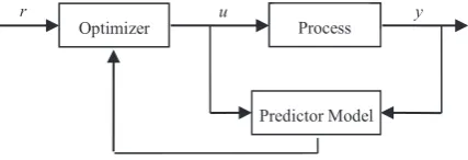
Figure 1 shows the general block diagram of model predictive control strategy. Contrary to the classical control which only uses past and present output or states of the plant, the model predictive control considers prediction of future signals as well. All the MPC algorithms have common components which are predictive model, cost function and calculation of future control to minimize the cost function.
)LJXUHThe general structure of MPC
Predictive model is a fundamental part of an MPC. At the first step, a mathematical model of the process is identified based on past inputs(ݑ(ݐ+݅);݅ െ1)
and past outputs (ݕ(ݐ+݅);݅ 0) . This model, together with future inputs (ݑ(ݐ+݇); 0 ݇ ܯ௨)is
employed to predict future outputs (ݕො(ݐ+݇|ݐ), 1 < ݇<ܯଶ). Since the future inputs are unknown, practically the model gives future outputs as a function of future inputs. At the next step, an optimization problem is solved using a cost function of predicted error and future control effort. A general expression for such cost function can be given as follows:
ܬ(ܯଵ,ܯଶ,ܯ௨) =σெమ ߜ(݇)[ݕො(ݐ+݇)െ ݎ(ݐ+݇)]ଶ
ୀெభ +σ ߣ(݇)[ȟݑ(ݐ+݇)] ଶ ெೠିଵ
ୀ (1)
where ݕො(ݐ+݇) is ݇ steps ahead prediction of the output, ݎ(ݐ+݇) is ݇ steps ahead reference signal,
ݑ(ݐ+݇)is ݇steps ahead control signal andȟis the
backward difference operator. ܯଵ> 1and ܯଶpresent interval of output prediction and ܯ௨ is the control
horizon. Normally, ܯଵ is equal to the delay of the
process [15]. Coefficients ߜ(݇) and ߣ(݇) affect performance of the controller and usually are considered to be constant.
Industrial processes are subject to some constraints in input signal, output signal, their differentiation through time, acceptable overshoot and so on. These
Optimizer u Process y
constraints can be dealt in MPC with minimization of Eq. (1) subject to defined constrains. Solution of this optimization problem is the future input to apply as control signal to the process. In order to obtain
ݑ(ݐ+݇), it is necessary to minimize the cost function
J. To do this, predicted outputݕො(ݐ+݇)is substituted in the cost function based on the prediction model as a function of previous and present inputs and previous outputs which are known and future control signal which is unknown [11].
Despite of the fact that most of industrial processes are nonlinear in nature, many applications of MPC so far have been applied to linear models [3]. However, there exist processes whose nonlinearities are severe enough not to be negligible. Accordingly, nonlinear model predictive control, NMPC which uses a nonlinear model in MPC strategy is very helpful and justifiable [14]. In nonlinear modeling, it is possible to use neural models, fuzzy models, a combination of both or other nonlinear models such as Wiener and Hammerstein models. In this paper, multilayer perceptron (MLP) neural network is selected as the process model.
To identify a nonlinear model, it is necessary to excite the system at different operating points. Acquired data are saved in a database to be used in identification ofthe plant. The structure of model (number of neurons), algorithm of parameter adjustment (training of neural networks), quality of produced data and preprocessing of data (noise elimination, delay estimation and so on) affect quality of the model [3].
Since in neural network training, mean of square of errors is used as the criterion of parameter adjustment, volume of produced data in any area heavily affects quality of identification in that area. If the number of data points in an operating point is much less than the number of data points in another operating point, the effect of modeling error for the first data set is less than that for the second data set in the cost function. This reduces the efficacy of the cost function on designing a good model for the first operating point, despite the error is considerable in this area. In fact, training algorithms have more tendencies to reduce small errors in regions with a large amount of data than to reduce large errors in regions with small amount of data.
'DWDVHSDUDWLRQE\IX]]\*DWK*HYD
FOXVWHULQJ
Identification data may be produced either actively using some special experiment or passively using the ordinary data of the process during its operation. In the first case, one may excite the process in different operating points and select necessary data in each one.
However, this may not possible in a plant during its normal operation. In this case, the only available data for identification is the ordinary data logged during the operation. These data include both frequent and infrequent data points. Therefore, it is necessary to separate data of different operating points and use specific ratio of them for identification, as will be presented in Section 4. For this purpose clustering is employed to separate frequent and infrequent data points.
There are various clustering methods [12]. C-means clustering is a basic method in which data are clustered in some hyper-sphere clusters. Gustafson-Kessel method was introduced in [9] in which the clustering distribution variation can be different in each direction which means each cluster is a hyper-ellipsoid. However, the total clustering error proportionally depends on the number of data points in that cluster in both of the above methods. Therefore,the total clustering error for a small size but scattered and high distributed cluster may be much less than the total clustering error for a condense but large size cluster. As a result, the clustering algorithm may divide the large cluster in two parts and includes small groups of data in each of these two large clusters to minimize the overall clustering error. Gath and Geva [7] presented another clustering in which the number of data points in each cluster is inversely affects the clustering error. Therefore, a small cluster may have the same effect in the overall clustering error as a large one with more or less the same distribution of data. In this section, fuzzy Gath-Geva clustering algorithm is used to cluster the data in frequent and infrequent operating points.
*DWK*HYDFOXVWHULQJ
Clustering is a nonsupervisory classification technique in which the data set is divided into ܿ
clusters based on the similarity of the members of each other and their difference from those of other clusters. Consider data set ܺ with data points
ݔ= (ݔଵ,ݔଶ, … ,ݔ),݅= 1,2, … ,ܯ, where ܯ is the number of data points in ܺand݈ is the dimension of
ܺ . The problem is to find ܿ cluster centers
ݒ=൫ݒଵ,ݒଶ, … ,ݒ൯,݆= 1,2, … ,ܿ, and membership of ݔto the cluster ܥsuch that an overall cost function
of distance of data from their cluster center is minimized. The distance function in fuzzy Gath-Geva clustering is defined as [7]:
ܬ=σ σ ݂൫ݔ
,ݒ൯݀ଶ൫ݔ,ݒ൯ ௩ೕא
௫א (2)
where ݀ଶ൫ݔ
,ݒ൯is the distance of ݔfrom center of
ݒ:
݀ଶ൫ݔ ,ݒ൯=
ଵ
ೕට݀݁ݐ൫ܣ൯݁ݔ ൬ ଵ
ଶ൫ݔെ ݒ൯ܣ ିଵ൫ݔ
݂൫ݔ,ݒ൯is the degree of membership of ݔto cluster
ݒwhich is computed during the clustering,݉is used
to change the fuzziness of the clusters andܣis the covariance matrix of cluster ܥ.ܲ is cardinality of
cluster ܥwhich is defined as the proportion of sum of
the membership values of all data points to ܥto sum of all membership values of all data points to all of the clusters.
&OXVWHULQJRIS+QHXWUDOL]DWLRQSURFHVV
pH neutralization process is selected to illustrate clustering frequent and infrequent operating points. pH process, as demonstrated in Figure 2, has three reaction streams: HNO3 as an acid, NaOH as a base and water. It has two output variables: liquid level and pH of the output stream. Water flow rate is deployed to control the liquid level and base flow rate is the control signal on pH control loop where acid flow rate is disturbance. A detailed model of this process is presented in [10] which is used in this study.
)LJXUHpH Neutralization process
)LJXUHThe titration curve of pH process
This process is a severe nonlinear process. Figure 3 shows a typical titration curve of a pH neutralization process. As it is shown in this figure, gain of the process could be categorized into 3 different areas; low gain in areas 1 & 5, medium gain in areas 2 & 4 and high gain in area 3.
If we design controller of this process in any area other than area 3, changing the operating point from that area to area 3 may result in oscillation or even instability. Suppose the pH process usually operates in area 2 but operates at a very small interval of time in area 3 due to some disturbances. Accordingly, we consider area 2 as the main or frequent area and area 3 as the rare or infrequent area. The question is how to separate data points of area 2 and 3 from each other.
Since dynamic behavior of processes is concerned in this paper, each data point consists of the regression vector used later in nonlinear identification of the pro-cess. This vector, as will be stated in sub-section 4.1, is ൫ݕ(ݐ),ݕ(ݐ െ1),ݕ(ݐ െ2),ݕ(ݐ െ3),ݑ(ݐ െ1),ݑ(ݐ െ2)൯,
where ݑ(ݐ)is the inlet base feed rate and ݕ(ݐ)is the outlet pH value. Suppose ܰଵ is the number of data
points in the infrequent area and ܰଶis the number of data points in the frequent area and ܰ=ܰଶ/ܰଵ. In
other words, ܰ is the ratio of period of time the process operates in the frequent area with respect to that of the infrequent area.
We apply an amplitude modulation pseudo random binary signal (APRBS) [18] with length ܰଵ= 2000
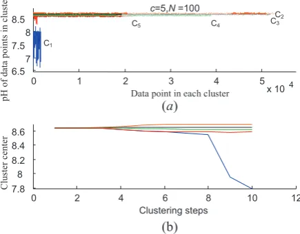
step. The amplitude of the inlet flow is selected so that the operating point remains in area 3. Another APRBS is also applied with different length ofܰଶand with the amplitude so that it operates in area 2. The regressor data are clustered using the Gath-Geva clustering method. Figure 4 illustrates the clustering result for
ܰ= 100 where the number of clusters is ܿ= 5.
Figure 4a shows the first element (the pH value) of each data point. The horizontal axis is the element number in each cluster. The clustering is near optimal after 10 training steps. Figure 4b illustrates the center of the clusters for these 10 steps of training. Although the number of infrequent data points is too small Gath-Geva clustering could accurately cluster them. The frequent data points are divided into 4 different clusters. To merge these clusters, we define a minimum threshold for the distance between the centers of the clusters.
)LJXUHClustering of pH neutralization process into 5
clusters
%DVH)HHG5DWH
S+
6
WHDG\
6
WDW
H
7LWUDWLRQ&XUYH
[
&
& & & &
&
Data point in each cluster
c N
pH of
data points
in clus
ter
s
point in ea
(a)
&OXVWHULQJVWHSV
C
lus
te
r c
en
te
r
1RQOLQHDULGHQWLILFDWLRQIRULQIUHTXHQW
RSHUDWLQJSRLQWV
The main question in simultaneous identification of frequent and infrequent operating areas is how to select the ratio of the data in these areas to identify them such that the following objectives are satisfied:
1. Identify the main operating area with a high quality such that the model error in this areaislow.
2. Identify the process in the infrequent area such that the model error in this area is not high.
3. The overall identification error of the model
over all the operating range is optimally low. To satisfy these objectives, we have to find the ratio of data to be employed for identification. In subsection 4.2, through several experiments, we will find the appropriate ratio. To this end, first we present some practical concerns in modeling of pH process in subsection 4.1.
In identification of pH process similar to other systems, several practical issues should be considered which are explained in details in [21]. One of the important factors in a good identification is quality of the identification data. Accordingly, the identification data need to be informative, i.e. excite different frequencies and operating points of the process dynamics. To this end, we use a binary signal with admissible amplitude to excite all modes of the system. Also, we add noise to that signal to increase the quality of identification and to have a better excitation. We consider the amplitude of noise roughly 1/15 of the signal amplitude. To collect data, open loop identification is employed which is acceptable due to stability of the pH neutralization process. Since the time constant of the process is 350 to 400 seconds, we select the sample time as 30 seconds. The input vector of the neural network consists of
ݕ(ݐ െ1),ݕ(ݐ െ2),ݕ(ݐ െ3),ݑ(ݐ െ1),ݑ(ݐ െ2) and its output isݕ(ݐ). The number of neurons is chosen based on an error threshold. Consequently, the neural network is composed of a hidden layer with 5 and, in some of experiments, with 7 neurons.
3UDFWLFDOFRQFHUQVLQS+SURFHVVLGHQWLILFDWLRQ
This section explains how the amount of required data in different areas is selected to satisfy the mentioned objective of simultaneous identification of frequent and infrequent operating points. In order to find the best ratios, we provide the following experiment. Suppose ܰis the ratio of period of time the system operates in the frequent areas with respect to that of the infrequent areas. After clustering, part of data in frequent cluster and part of that from the infrequent cluster is selected to identify the plant. If we select ݊ଵand ݊ଶas the numbers of training data
sets in infrequent area and frequent area, respectively, then ݊=݊ଶ/݊ଵis the ratio of training data sets. In our experiment, for different values of ܰwe identify the
process with different value of݊. Also, another data set is used as test data set, which its ratio is ܰଶto ܰଵ
as well, to measure the infrequent data error, frequent data error and the total error in each case. Table 1 compares MSE1, MSE2 and MSET which are mean
square of identification errors of infrequent data, frequent data and total data sets, respectively, for different values of݊and ܰ.
As depicted in the table, if for example the length of the infrequent operating area of the process is one tenth of that of the main operating area and the ratio of the training sets for the main and the infrequent data sets is selected as 2 to 1, then the total error of the performance of the test data in the infrequent operating point is equal to 0,86 × 10ି. Figures 5, 6,
and 7 show MSE for infrequent operating point, main operating point and total operating points for different values of nand N, respectively.
In Figure 5, we observe that by increasing ݊, the error associated with the infrequent operating point increases. In fact, the ability of the neural model to predict the output of the infrequent operating point decreases due to decrease of proportion of data in this operating point to the main operating point in the total data. However, in all of the error curves in Figure 5 up to݊ 25, the MSE of data in the infrequent operating point has a negligible value and performance of the modelis acceptable.
)LJXUHIdentification error of the infrequent operating
point for different values of Nand n
As it can be observed from Figure 6, the error decreases for the main operating point by increasing the proportion of data ofthe main operating point to the infrequent operating point for all different values of ܰ. This is because the neural network model better identified the main operating point. Hence, the error associated with this area decreases. However, the rate of this decrease for lower ratios is rapid and for larger ratios is very slow. In all the error curves for ݊ 12
this rate is very slow and approximately equal to zero. By studying Figure 7, we observe that MSE value for data sets associated with the combination of infrequent and main operating points initially
n
MS
E1
N=1
N=5 N=10 N=20 N=50 N=100 N=200 N=500
7DEOHThe identification MSE for total data set, infrequent data set and frequent (main) data set (all values are in 10-6)
)LJXUHIdentification error of the main operating point for different values of Nand n
decreases with slow rates and then increases with rapid rates. Hence, to minimize the error cost function, the appropriate ratio is in an interval around the optimal point.
)LJXUHIdentification error of the total operating points for
different values of Nand n
According to Figures 5 to 7, we can conclude that for the main operating point, the ratios greater than 12 and for the infrequent operating point the ratios less than 25 are acceptable. Therefore, the common
n
MS
E2
N=1 N=5 N=10 N=20 N=50 N=100 N=200 N=500 N=1000
n
MS
ET
N=1 N=5 N=10 N=20 N=50 N=100 N=200 N=500 N=1000 N
n 1 2 3 5 7 10 12 15 20 25 30 40 50 70 100 150 200 500 700 1000
1
MSET0.4706 0.4758 0.4749 0.4645 0.469
MSE10.8198 0.8553 0.8602 0.843 0.8529
MSE20.1215 0.0962 0.0896 0.086 0.0852
5
MSET0.2278 0.221 0.2252 0.2125 0.2144 0.1486
MSE10.8187 0.8541 0.8993 0.8377 0.8518 0.8634
MSE20.1099 0.0947 0.0906 0.0877 0.0872 0.0773
10
MSET 0.188 0.155 0.1485 0.1469 0.1477 0.1486
MSE1 1.07 0.8565 0.8219 0.8381 0.8525 0.8636
MSE2 0.1 0.085 0.0813 0.078 0.0774 0.0773
20
MSET0.1403 0.1278 0.1246 0.1206 0.1208 0.1211 0.1216 0.1217 0.1224
MSE10.8189 0.8524 0.8707 0.8346 0.8537 0.8616 0.8734 0.8739 0.8874
MSE20.1065 0.0917 0.0873 0.085 0.0843 0.0842 0.0841 0.0842 0.0843
50
MSET0.1348 0.1148 0.1106 0.1069 0.1064 0.1064 0.1065 0.1066 0.1065 0.1067 0.135 0.139 0.141
MSE10.8378 0.8534 0.8618 0.8481 0.8569 0.8633 0.8724 0.8721 0.868 0.8724 2.316 2.523 2.602
MSE20.1208 0.1001 0.0956 0.0921 0.0914 0.0913 0.0912 0.0913 0.0913 0.0914 0.092 0.092 0.092
100
MSET 0.117 0.099 0.0965 0.0934 0.0937 0.0929 0.093 0.093 0.0932 0.0931 0.0928 0.0925 0.0923 0.6 0.73
MSE1 0.829 0.8453 0.858 0.8429 0.8992 0.8635 0.8733 0.8676 0.8898 0.8721 0.8529 0.83 0.8094 51.84 65.77
MSE20.1099 0.0916 0.0889 0.0859 0.0857 0.0852 0.0852 0.0853 0.0853 0.0853 0.0853 0.0852 0.0851 0.0851 0.0856
200
MSET0.1112 0.0958 0.092 0.0888 0.0882 0.0881 0.0881 0.0882 0.0882 0.0883 0.0881 0.0881 0.098 0.34 0.43 0.9 1
MSE10.8198 0.8553 0.8602 0.843 0.8563 0.8635 0.8742 0.8734 0.8682 0.8711 0.8458 0.8317 2.748 50.69 70.33 156 174.7
MSE20.1077 0.092 0.0881 0.085 0.0844 0.0843 0.0842 0.0843 0.0843 0.0844 0.0843 0.0843 0.084 0.084 0.084 0.084 0.088
500
MSET0.1128 0.0978 0.0944 0.0906 0.0899 0.0897 0.0897 0.0898 0.0898 0.0898 0.0897 0.093 0.093 0.19 0.2 0.4 0.4 0.5
MSE10.8189 0.8524 0.903 0.8346 0.8537 0.8616 0.8734 0.8739 0.8874 0.862 0.8531 2.521 2.637 51.39 57.17 162.4 166 231.5
MSE20.1114 0.0963 0.0928 0.0891 0.0883 0.0882 0.0881 0.0882 0.0882 0.0883 0.0882 0.089 0.088 0.088 0.088 0.088 0.088 0.088
1000
MSET0.1393 0.1249 0.1216 0.1188 0.1177 0.1174 0.1174 0.1175 0.1175 0.1174 0.1174 0.1173 0.119 0.17 0.18 0.3 0.3 0.3 0.4 1.9299
MSE10.8187 0.849 0.8737 0.876 0.8545 0.863 0.8737 0.8718 0.8884 0.8613 0.8527 0.8301 2.606 50.49 66.5 154.9 173.9 215.4 245.5 1800
interval of [12,25] is acceptable. Nevertheless, for
ܰ< 12we can set ݊=ܰ.
Thus, we find an appropriate value for the ratio of the identification data of the main operating point to that of the infrequent operating point for the pH process such that the modeling objectives are satisfied. In fact, through this selection, despite reduction of amount of selected data from the main operating point, MSE does not increase significantly. On the other hand, the model is sufficiently trained in the infrequent operating area to improve not only the model in this area but also the overall performance of the system.
As a consequence, the overall nonlinear identification of a process in frequent and infrequent operating points can be summarized in the following steps:
6WHSGather the actual data of the process during its operation.
6WHSCluster the data using hierarchical Gath-Geva fuzzy clustering.
6XEVWHS If standard deviation of any of the clusters is high, divide it into smaller clusters.
6XEVWHS If centers of some clusters are close to each other, merge these clusters.
6WHSSelect part of data of each cluster for identification according to the following ratio rule:
5DWLRUXOH If actual ratio of data between clusters is less than 25, use the same ratio of data for identification; otherwise use some ratio between 12 to 25.
6WHSIdentify the nonlinear model using the selected data.
1RQOLQHDUQHXUDOPRGHOSUHGLFWLYHFRQWURO
In the previous section, we found an optimal interval for ratio of the main data to the infrequent data when a nonlinear model is identified for both operating points. In this section, we use this ratio to train a neural network to identify a nonlinear model of the process to be used in an NMPC structure.
The actual ratio of data is supposed to beܰ= 1000 . In the identification process we selected different training ratios as ݊= 1, 15and1000. Then, each of the identified models for any of these ratiosis used in the model predictive control structure. The closed loop tracking results for these controllers are shown in Figures 8 to 10. In these figures, the plant is in infrequent operating area during the first 2000
sample times. After that it works in the main operating area for 2,000,000sample times, however just portion of it is shown in these figures. MSE values of reference input tracking for neural model predictive control using different models are given in Table 2.
7DEOH MSE of tracking in NMPC for different ratios of training data sets (all values are in 10-6).
n 1 15 1000
MSET 3.48 0.90 0.98
MSE1 31.66 22.68 135.20
MSE2 3.46 0.88 0.84
Figure 8 illustrates the case ݊=ܰ= 1000, i.e. the training data ratio is the same as the real data ratio. As it is shown, the output response in the infrequent operating area is oscillating. The reason is that, only one thousand of the training data are from infrequent operating point. This means that this area has not been accurately identified. So the model is not suitable for this area and the NMPC cannot control the process in this operating point. When the same number of data points are selected for both main and infrequent operating areas, i.e. ݊= 1, the results given in Figure 9 are obtained. The response is stable in all the operating points. However, comparison of the results of main operating points in Figures 8 to 10 shows that the quality of the controller degrades. This is also depicted in Table 2, where the MSE of the main operating area with ݊= 1is 4 times more than the MSE for the same area when ݊= 1000.
The results given in Table 2 illustrate that the controller performance is the best when݊= 15. For the main operating area, increasing n from 1 to 15 results in a significant improvement in the MSE. However, more increase of this ratio to ݊= 1000
does not have a large effect on the performance of this area. On the other hand, increasing ݊from 15 to 1000 significantly degrades the performance of the infrequent operating area. MSET values recommend
that ratio 15 is also the best ratio among the others for the total test data set. Summarizing the above results, we conclude if the identification (or training) data ratio is selected as ݊= 15, all three objectives of Section 2 would be satisfied. It is important to emphasize that there is no large difference between the results when ݊is any value between 12 and 25. This means that the results are robust and are not largely sensitive to the ratio values.
&RQFOXVLRQV
)LJXUHNonlinear model predictive control with training ratio of ݊= 1000
)LJXUHNonlinear model predictive control with training ratio of ݊= 1
nonlinear model predictive control, heavily depend on the identified model. Therefore, deviation of the model from the actual behavior of the plant degrades performance of such controllers. Using low number of data point in infrequent operating space causes significant inaccuracy in that space which may end to instability. On the other hand, using the same number of data points in both frequent and infrequent operating points, causeslow accuracy in most of the
time which reduces the overall efficiency. To resolve this problem, in this paper we proposed to choose an appropriate data ratio of the main operating area to that of the infrequent operating area in the identification.
The usual assumption in system identification is that we should design the excitation signal according to important frequency range and, in nonlinear identification also according to different operating
6DPSOHV 1RQOLQHDU 3UHGLFWLYH
\VS
\
6DPSOHV
X
6DPSOHV 1RQOLQHDU 3UHGLFWLYH
\VS\
6DPSOHV 1RQOLQHDU 3UHGLFWLYH
\VS
\
6DPSOHV
X
6DPSOHV 1RQOLQHDU 3UHGLFWLYH
)LJXUHNonlinear model predictive control with training ratio of݊= 15
points [18]. However, to identify part of a process in a working factory, we are not allowed to apply our designed excitation signal due to some technical safety and conservatism. Therefore, we have to use the usual data of the process which is logged into historical data servers. These data come from different operating points with different data ratio and different importance. So, to apply the above suggested data ratio, it is necessary to distinguish various operating points. We use clustering for this purpose. This is not new, but since it is supposed that the amount of data points in various data sets are substantially different, usual method of clustering cannot properly cluster the data sets. We suggest using Gath-Geva clustering method. In addition, to improve its performance a hierarchical algorithm is presented for it.
We showed that for the pH neutralization process, which is a highly nonlinear process, by selecting data ratios between 12 and 25, in addition to high accuracy of the identified model in the main operating area, modeling error in the infrequent operating area does not exceed a specific threshold. Besides, error associated with the total data is minimized as well when this data ratio is selected. Since the ratio interval is somehow wide, the algorithm is robust to the selection of the data ratio.
Although nonlinear model predictive control of a pH neutralization process is studied in this paper as a case study, the idea of selection of specific ratio for identification of a nonlinear process can be used in other types of model based nonlinear control and processes. Also, using a neural network for model
structure is not crucial. Using any other kind of black box nonlinear models has the same problem. So the same algorithm can be applied to them for nonlinear system identification in both frequent and infrequent operating points.
5HIHUHQFHV
[1] %0 $NHVVRQ +7 7RLYRQHQA neural network model predictive controller In: Journal of Process Control, 2006, Vol. 16, pp. 937-946.
[2] 7/ $OL\HY $7 6WDPSV (3 *DW]NHImproved crude oil processing using second-order Volterra models and nonlinear model predictive control. In: American Control Conference, Seattle, USA, Jun. 11-13, 2008, No. 11-13, pp. 2215-2220.
[3] () &DPDFKR & %RUGRQV Model predictive control, Springer-Verlag, Berlin, 1999.
[4] %$ )RVV 7$ -RKDQVHQ $9 6¡UHQVHQ
Nonlinear predictive control using local models - applied to a batch fermentation process. In: Control Engineering Practice, 1995, Vol. 3, pp. 389-396. [5] .3 )UX]]HWWL $ 3DOD]RJOX .$ 0F'RQDOG
Nonlinear model predictive control using Hammerstein models. In: Journal of Process Control, 1997, Vol. 7, No. 1, pp. 31-41.
[6] 9 *DOYDQDXVNDV Adaptive pH control system for fed-batch biochemical processes. In: Information Technology and Control, 2009, Vol. 38, No. 3, pp. 225-231.
[7] , *DWK $% *HYD Unsupervised optimal fuzzy clustering. In: IEEE Transaction on Pattern Analysis and Machine Intelligence, 1989, Vol. 11, pp. 773-781. 6DPSOHV
6DPSOHV 1RQOLQHDU 3UHGLFWLYH
\VS
\
6DPSOHV
X
S 1RQOLQHDU 3UHGLFWLYH
[8] $ *UDQFKDURYD - .RFLMDQ 7$ -RKDQVHQ
Explicit output-feedback nonlinear predictive control based on black-box models. In: Engineering Applications of Artificial Intelligence, 2011, Vol. 24, No. 2, pp. 388-397.
[9] '(*XVWDIVRQ:&.HVVHOFuzzy clustering with a covariance matrix. In: Proc. IEEE Conference on Decision & Control, San Diego, USA, 1979, pp. 761-766.
[10]0$ +HQVRQ '( 6HERUJ Adaptive nonlinear control of a pH neutralization process. In: IEEE Trans.
Control Systems Technology, 1994, Vol. 2,
pp. 169-182.
[11]+%+XR ;-=KX :4+X +<7X -/L -<DQJNonlinear model predictive control of SOFC based on Hammerstein model. In: Journal of Power Sources, 2008, Vol. 185, pp. 338-344.
[12]$. -DLQ 01 0XUW\ 3- )O\QQ Data Clustering: A Review. In: ACM Computing Surveys, 1999, Vol. 31, pp. 264-323.
[13]$ -D]D\HUL $ )DWHKL + 6DGMDGLDQ $ .KDNL6HGLJK Disturbance rejection in neural network model predictive control. In: 17th IFAC World Congress, Seoul, Korea, July 6-11, 2008. [14]%.RXYDULWDNLV 0&DQQRQ Nonlinear predictive
control: theory and practice. In: Institution of Engineering and Technology (IET), 2001.
[15]-0 0DFLHMRZVNL Predictive control with constraints, Prentice-Hall, N.J., 2002.
[16]6 0DKPRRGL - 3RVKWDQ 05 -DKHG0RWODJK $0RQWD]HULNonlinear model predictive control of a pH neutralization process based on Wiener-Laguerre
model. In: Chemical Engineering Journal, 2009, Vol. 146, pp. 328-337.
[17]%0DQHU)-'R\OH%$2JXQQDLNH5.3HDUVRQ
Nonlinear model predictive control of a multivariable polymerization reactor using second-order Volterra models”, Automatica, 1996, Vol. 32, pp. 1285-1301. [18]2 1HOOHVNonlinear system identification,
Springer-Verlag, Berlin, 2001.
[19]01RUJDDUG25DYQ1.3RXOVHQ/.+DQVHQ
Neural networks for modeling and control of dynamic systems, Springer-Verlag, Berlin, 2003.
[20]5. $O6H\DE < &DRNonlinear model predictive control for the ALSTOM gasifier. In: Journal of Process Control, 2006, Vol. 16, pp. 795-808.
[21](3H\PDQL$)DWHKL3%DVKLYDQ$.KDNL6HGLJK
An Experimental Comparison of Adaptive Controllers on a pH Neutralization Pilot Plant. In: IEEE Conference & Exhibition on Control, Communication and Automation (INDICON), Kanpur, India, 11-13 Dec. 2008.
[22]965 5DR 53LFNKDUGW 0&KLGDPEDUDP '6ZDWLNonlinear Control of pH System for Change Over Titration Curve. In: Chemical and Biochemical Engineering Quarterly, 2005, Vol. 19, No. 4, pp. 341-349.
[23]%9DWDQNKDK $)DWHKL $.KDNL6HGLJK Neural Network Model Based Predictive Control for Multivariable nonlinear systems. In: International
Multi Conferences on Systems and Control,
Yokohama, Japan, Sep. 7-10, 2010.