M
ARKET POWER IN POWER MARKETS
:
T
HE
CASE OF
F
RENCH WHOLESALE ELECTRICITY
MARKET
SOPHIE MERITET
University of Paris Dauphine, France
THAO PHAM
University of Paris Dauphine, France
ABSTRACT
The French wholesale market is set to expand in the next few years under European pressures and national decisions. In this paper, we investigate the performance of the French wholesale power market to examine whether or not the equilibrium outcomes are competitive. After a literature review on the different existing models, an extension of the Bresnahan - Lau (1982) method in panel data framework is employed with hourly dataset during 2009-2012 on the French wholesale market. The model-based results suggest that though market power is found statistically significant in several peak-load hours, it stays at very low level. On average, no market power is exercised over the examined period. These results correspond with the extremely regulated wholesale power market in France. It is of high interest given the future evolution of the French wholesale market which will be among the biggest in Europe in 2016 after the end of regulated tariffs for all firms.
Keywords:
Electricity, market power, France, oligopolistic market, panel data.
JEL classification:L13, D47, C22, C51
CORRESPONDING AUTHOR:
Sophie Meritet, LEDa-CGEMP University of Paris Dauphine,FRANCE
1. INTRODUCTION
The electric power sector worldwide has experienced an exceptional policy trends that fundamentally reshaped the industry over the last 20 years: liberalization and deregulation, or more generally "electricity reform". This policy refers to a transition from economic model of “vertical integration monopoly under regulation” to a market-based system with regulatory restructuring. Reforming the electricity industry was much harder than it appeared at the first glance. One cannot simply break up the monopoly, cease to regulate and wait for the market forces to rush in making competition work. One of the problems arose from the shift to reliance on market prices instead of regulated tariffs for electric generation has been market power.
"Market power" is not a new and recent concept. It is defined in economics as the ability to alter profitably prices away from competitive level, i.e., the marginal cost level. Theoretical and empirical studies of "market power in electricity markets" however, have only been developed recently. It raises concerns in both sides of the Atlantic, as regard to the way of defining, detecting, and monitoring it. Up to the late 1980s, empirical studies of market power in liberalized generation electricity markets are scarce since it had rarely been contemplated outside the United States (Borenstein [2000]). Most studies had attempted to assess the potential for exercising market power by measuring the extent of market concentration in regional submarkets. Studies in Europe were developed a bit latter but were not out of this line. However, over the last 10 years, market power detection techniques have dynamically evolved, varying enormously from theoretical to empirical models, from market structure to market outcome approaches; from direct to indirect estimations, etc. Indeed, the issue arose for any attempt to assess market power level has been the calibration of marginal cost levels.
offered by suppliers with market prices will increase. That is why the French wholesale market should become more liquid with more participants in the near future. It is highly relevant to study the wholesale electricity prices in France at this stage. Indeed, there have been some doubts provoked in electricity market in France on the issue of market power as Electricité de France (EDF), the biggest producer of electric power in Europe, still dominates the domestic market after the reform. Moreover, despite the market opening, wholesale prices in France have drastically increased: the index of Powernext Baseload Forward Year Ahead almost tripled between 2004 and 2008, increasing even faster than oil price. The wholesale prices in France have been increasingly higher than those in Germany since the end of 2012 after a long period of strong price convergence between the two markets.
This paper analyzes the level of competition in the French wholesale markets. The extended Bresnahan-Lau [1982] model is conducted using the data from the French spot market during 2009-2012. In particular we attempt to address several issues which are still debatable in market power modelling, for example, the unknown accounting datum of economic marginal cost and the treatment of hourly data on electricity spot prices.
The paper proceeds as follows. In the first section, we present different models to investigate the exercise of market power in power markets that have been employed in literature. The second section describes the French electricity markets with a focus on the wholesale one. The third section explains our model which is an extension of Bresnahan-Lau [1982] and the data we used. The fourth section provides the results and some analysis. The last section concludes.
The fourth section provides the results and some analysis. The last section concludes.
2. DIAGNOSING MARKET POWER IN ELECTRICITY MARKETS
2.1 Electricity is a specific "good"
Electricity market exhibits unusual characteristics that make exercising market power particularly likely. First, the inelasticity of demand by prices in short term is one of fundamental flaw. Indeed, electricity is an essential good with very low elasticity of demand and most of the customers do not have means to respond to real time price. Second, several technical attributes in electricity make diagnosing market power particularly challenging. In fact, electricity cannot be stored economically on a large scale. The implication is that when capacity is tight, demand exceeds the maximum capacity there is no storage available, even a supplier with 1% of total output can have incentive to exercise market power (pivot actors). Furthermore, electricity is transmitted over a network and follows laws of physics.
whether an abnormal high price is resulted from exogenous factors or abuse of market power. Any attempt to estimate market power in electric power markets needs to take into consideration theses specific features of electricity.
2.2 Literature review on diagnosing market power in power markets
Market power detection techniques developed over the last 10-15 years in the power markets vary enormously from theoretical to empirical models, from market structure to market outcome approaches; from direct to indirect estimations, each of which has strengths and weaknesses. Up to present, though there is still no definitive method for diagnosing market power in power industry, a lot of advances have been made.
The first attempt of empirical studies in market power was developed in the 1930s, known as Structure Conduct Performance approach (SCP). It holds that an industry's performance depends on the conduct (behavior) of sellers and buyers, which depends on the structure of the market. The structure is often summarized by market share or the relative market shares of the largest firms (Herfindahl-Hirschman Index-HHI). Though these indices are likely to serve as a potential screening of market power in long term ex-ante studies, there is very little empirical evidence supporting the application of these indices in predicting market power in electricity markets (Twomey, Green, Neuhoff and Newbery [2006]). In fact, they ignore many factors that contribute to the potential exercise of market power particularly demand conditions. In electricity market where demand and supply conditions can change rapidly, these static indices are not appropriate measurement of market power.
The Pivotal Supplier Index (PSI) and Residual Supply Index, designed particularly for electricity market by California ISO in 2002 (Sheffrin [2002]), are alternative structural indices which address some weaknesses of the classical concentration indices by taking into account the demand-side conditions. They measure the extent to which a generator's capacity is indispensable to supply the market after taking into account other generators' capacity. These indices, though being recently introduced, are increasingly applied in the US as a tool for market power analysis. However, the difficulties in defining the relevant markets still remain. And, like other structural indices, they only reveal the information about the potential of market power, not the actual level of market power exercise.
constraints in constructing the residual demand curves. Such constraints would decrease the residual demand elasticity and thus increasing the potential to exercise market power. Ignoring this factor might lead to underestimate the level of market power.
Perhaps the most sophisticated means of measuring market power have been involving market simulation models. While SCP studies focus on the question of "what causes market power" with assumption that the level of this market power is known, market simulation models take market power as an unknown factor and attempt to measure it. Named in different ways and implemented in different methods from simplest to the most complicated, the decisive clue of this approach concerns the estimation of marginal cost and oligopoly equilibria in different wholesale electricity markets. Direct estimation of marginal costs is derived from engineering data of fuel costs - the main cost component for nuclear and fossil fuel plants - and of heat rate-the efficiency with which fuel is converted into energy. Multiplying the heat rate with fuel prices allows reliable estimation of the fuel cost component. The system benchmark price and quantity equilibrium is then found by two categories of models : the first approach concerns optimization/simulation models as done by for example Boweret al. [2001], Bushnell and Saravia [2002], Green [2004], Lang and Schwarz [2006], Müsgen [2006], Weigt and Von Hirschhausen [2008], Competition [2007], Möst and Genoese [2009]; the second ones with various oligopoly models such as supply function equilibrium done by Green and Newbery [1992], Halseth [1999], Arellano [2003], or simple Cournot - Bertrand - Nash equilibrium as done by a series of papers of Borenstein and Bushnell [1999] , Borenstein, Bushnell and Wolak [2000] in Californian electricity market.
These models have been applied to many electricity markets throughout the world because they are firmly-grounded in oligopoly theory. However, they are intractable in empirical estimation because they require a proper calculation of marginal cost. Weigt and Von Hirschhausen [2008] show that the non-linear complexity of electricity pricing makes it difficult to design a realistic model. As pointed out by Harvey and Hogan [2002] every model has some level of uncertainty and thus produces a range of possible outcomes. In fact, the common approximation of assimilating the variable costs of fuels and plant performance seems unsatisfactory in many cases, particularly for nuclear power generation and hydropower whose variable costs are close to zero but opportunity costs might be very high. This is the case in French electricity market where the merit curve has a particularly flat-shaped due to the large part of nuclear power in the generation mix (over 85%). This makes the calibration of price-cost margins less reliable and thus negates the certitude of conclusions.
3. FRENCH MARKET DESIGN
3.1 The French energy situation
The energy sector in France has changed dramatically since the first oil shock in 1973 and the government’s decision in March 1974 to increase the nuclear power capacity rapidly. Following this decision, the use of coal and oil declined markedly, substituted mainly by the growth in electricity and natural gas consumption. Today, France is the eighth largest producer of electricity in the world and the second in term of nuclear production. Contrary to several European countries which benefit from an abundance of raw materials, France is poor in energy resources (Meritet [2007]). Between 1973 and 2012, electricity consumption almost tripled despite a minor decline in the years 2009 and 2011 (due to the economic crisis and weather conditions). Without fossil fuel reserves, the civil nuclear power program led to a substitution in electricity generation. The increase in nuclear power generation (15TWh in 1973 to 405TWh in 2012) is therefore accompanied by a reduction of the use of classic thermal units. Today, France represents 17% of the nuclear power generation in the world with 58 reactors. EDF, the former vertical integrated public monopoly, controls 80% of the country’s power generating capacity including all atomic reactors, two-thirds of thermal capacity, 81% of hydroelectric capacity and about a third of renewable output.
The French energy mix points to a large consumption of oil (used especially in transport) and nuclear power. In 2012, 75% of electricity was generated by nuclear power plants and 12% by hydro plants which are used for base load in the merit order. The residential sector is the country’s largest electricity user, currently representing about two thirds of the total. Next in importance is the industrial sector. The French nuclear electricity production amounts to 63 130 MW in 2012; the rest is 6 160 MW for coal plants, 5 009MW for natural gas, 6 945MW for fuel and peak load, and 24 301MW for hydro. The demand was divided up as follows: residential and services 67.3%, industries 28.1%, transport 2.8% and agriculture 1.7%.
While French consumption is the second largest in Europe after Germany (in terms of number of consumers and in output), its power trading market is not as dynamic due to the limited number of market players. It can also be particularly constrained in winter, since French demand is very sensitive to temperature. In 2012, for example, the level of electricity consumption reached more than 102 000MW on February 8, the highest recorded level in France. A one degree drop in the temperature is estimated to increase the 7 pm electricity demand peak of up to around 2 300MW. When temperatures are very low, France may not have enough installed capacity, it has to import power from the neighboring countries in order to guarantee the supply.
3.2 The French wholesale market
regulated tariffs for small businesses on retail market planned in 2016 by the 2000 NOME Law (New Organization of Electricity Market).
One particular characteristic of French wholesale power market is an overlap of different types of prices and tariffs, which are resulted from a number of regulatory instruments - the government's attempt to reconcile the economic, social, and political contradictions.
With the gradual market opening since 2000, a certain number of "eligible consumers" decided to quit the system of regulated tariff to participate in the system of competitive prices on the market which, at that time, was relatively low (see figure 1). This choice was, however, irreversible.
Source: Authors, based on data from EPEX, CRE, Eurostat
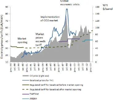
Figure 1. Evolution of French electricity prices and tariffs (1998-2012)
ta from EPEX, CRE, Eurostat
were, therefore, little impacted by the increase of fossil fuels prices or the implication of CO2 prices since 2005. On the other hand, market prices reply to all these changes. In fact, market prices are set equal to marginal cost of the last plant mobilized to fulfil the demand (marginal plant). If the French electricity system was isolated, i.e., no exchanges with neighboring systems, the nuclear plants would be the marginal plants for almost 50% of time and the market prices would be generally set based on marginal cost of nuclear power; the gap between regulated tariffs and market prices thus would be shortened. However, with market opening and interconnexion between France's and neighboring countries' network, the marginal plants of production necessary to satisfy the demand of interconnected zone are thus most of the time coal or gas plant. The market prices align to the production cost of these plants, which, in turn, vary with the volatility of fossil fuel prices.
Figure 1 illustrates also the correlation of electricity market prices and crude oil prices - the leading price in energy sphere1. The surge of crude oil prices from 2004
leads to an increase of the two other fossil fuels' prices: coal and gas, and thus, have some impacts on electricity market prices. Therefore, although a coal or gas plant represents a very small part of total generation in France, the production cost of this plant will still become the reference price for the market because it is connected with other markets like Germany or Italy where half of electricity is produced from coal and gas. During peak load, electricity is imported from, for example, Germany and the prices would align to the gas plant which is relatively expensive. During the base load, electricity is exported to Germany. Even if the prices correspond to certain marginality of nuclear in France, the coal-fired plants which function almost all the time in Germany could influent market prices in France. The price convergence between France and Germany has been even more significant since the creation of market coupling contracts in the Central western European which covers Benelux, France and Germany in November 2010.
The great divergence between market price and regulated tariff had made the consumers having quitted the regulated system manifest their malcontent toward the liberalization (generally competition would have induced lower price). This contradiction led the French Government to authorize, by a law on energy in 2006, that the consumers having quitted the tariff can return to the protective tariff system - the so called TARTAM, the transitional market adjustment tariffs2 or, more
prosaically "tariff of return". The TARTAM is calculated from the regulated tariff, increased by 10 %, 20 %, or 23% matching with a mechanism of compensation ex-post3.
1 The evolution of natural gas and coal prices is highly correlated with the oil prices largely because
they are substitute in the power and heating markets; high price differences cannot remain for long. Indeed, natural gas is frequently purchased by long term contracts which contain a price clause setting an automatic link between gas price and the price of petroleum products.
2 Tarif réglementé et transitoire d'ajustement au marché
3 The TARTAM is considered as a Government aid for big enterprises and set with a mechanism of
The juxtaposition of regulated tariff, TARTAM, and market prices, as well as the conditions of irreversibility between regulated and market offers caused even more contradictions. Two clients having the same consumption profile do not have access to the same tariff offers. The incoherence of pricing system made market prices now too far from being a signal for new investment. Besides, the new entrants could hardly compete with the actual regulated tariffs, which reflect the amortized production cost of nuclear power of the incumbent to which its competitors have a priori no access. A new contradiction was provoked: competition is generally expected to lower prices but to promote competition in French electricity market, we need to raise the prices.
It was in these conditions that a law on new organization of the electricity market - the NOME law4 was enacted in December 2010. This law aims to enhance the
competition by abolishing gradually the regulated tariffs and the TARTAM. Furthermore, by this law, the incumbent EDF has obligation to sell part of its nuclear production to its competitors at a regulated price fixed by the regulator - ARENH, Regulated access to historical nuclear energy5. The ARENH price was
settled by the government at 40 €/MWh at start to be coherent with the TARTAM (from the 1st July 2011) then 42€/MWh from the 1st January 2012.6
Although the co-existence of spot prices and regulated tariff system should not have a great impact on the merit order, it reduces the market's liquidity and could make the spot prices more sensitive to supply/demand variations.
4. MODELING MARKET POWER
4.1 The Model
In an oligopolistic market of a few supply firms producing a homogeneous product with is supply of the ith firm, Q is the total supply equal to the total
demand ( ∑ ), the price elasticity of demand is retrieved from the aggregate demand function:
( ) (1)
with X is a vector of exogenous variables affecting demand, is a vector of parameters of demand function to be estimated and is error term.
System marginal cost function takes the form:
( ) (2)
where W is a vector of exogenous variables on the supply side (factor price), is vector of parameters of supply function and is error term of supply function,
MC(.) is marginal cost function. When firms are price takers, i.e. market is competitive, prices equal marginal costs, equation (2) holds, the system marginal cost curve is as same as market supply curve.
4 Nouvelle Organisation du Marché de l'Electricité 5 L'Accès Régulé à l'Électricité Nucléaire Historique
6 The ARENH price is prosaically regulated price at the wholesale level. It is established, according to
Bresnahan (1982) and Lau (1982) suggest that we use a conduct parameter, to nest various market structures7. For example, when firms are not price takers, it is
perceived marginal revenue, not price, will be equal to marginal cost. The industry supply relation will no longer be determined by (2) but takes the form:
( ) ( ) (3)
where P+h(.) is marginal revenue and ( ) is marginal revenue as perceived by the firm and ( ) ( )
⁄ . is now a new parameter indexing
the degree of market power. In perfect competition, and price equal to marginal cost, equation (2) holds. gives perfect cartel, and intermediate 's correspond to various oligopoly solution concepts.
Bresnahan(1982) and Lau(1982) give conditions on the functional form such that is identified by introducing a vector Z, entering the model to both shift the demand curve and change the slope of demand curve. The supply relation (3) is written in linear equation as:
(4)
By treating and as known (by estimating the demand equation), is now identified8. The economic intuition behind this is quite straightforward. The rotation
of demand curve around equilibrium will have no effect under perfect competition: supply and demand curve meet at the same equilibrium point before and after rotation. However, under either oligopoly or monopoly, firms with market power will see that elasticity of demand is changing, they will adjust both their conjectures about other rivals' behavior and their perceived marginal revenue then equilibrium price and quantity will respond. Thus, the market power parameter is identified.
Bresnahan-Lau in a dynamic framework
Steen and Salvanes [1999] propose a dynamic reformulation of the BL model in an error correcting model and Hjalmarsson [2000] uses the same dynamic concept but in an autoregressive distributed lag ADL model. A general argument in favor of using a dynamic model is that it takes into account both short run and long run
7 An alternative is to use non-nested hypotheses tests: see Gasmi and Vuong (1991) and Gasmi,
Laffont, and Vuong (1992)
8 The inclusion of the rotation variable PZ in the demand function is crucial for the indentification of
market power degree. To see this, denote
; is identified as the coefficient of Q*
estimates. The demand function (1) and supply relation (4) can be written in ADL framework:
∑ ∑ ∑ ∑
(5)
∑ ∑ ∑ ∑ (6)
where the long-run parameters are given as:
∑
∑ (7)
h(.) in (3) can be written as:
( ) (8)
And
∑
∑
∑
∑
∑
∑ (9)
The ADL formulation provides both a short-run measure of market power: and a long-run measure, . The demand function (5) incorporates an adjustment speed, ∑ , which measures the impact on of being away from the long-run target. The supply relation in (6) incorporates also adjustment costs and allows short-run deviations from the requirement that marginal cost should equal perceived marginal revenue (Steen [2003]).
5. MODEL SPECIFICATION AND THE DATA
5.1.1 The nature of data and specification for different model considerations
As discussed in section 2, electricity industry exhibits a distinguished feature which makes modelling it different from other markets. Due to the combination of strong variability of demand for electricity and non-storability of electricity, there exist 24 different prices for 24 hours per day. Any attempt to model electricity price should take this into account. There have been three broad modeling strategies of electricity spot prices in the existing literature9:
9 Except for Steen [2003] and Bask et al. [2011], those papers do not necessarily concern market
Modeling of the daily/weekly average price: Koopman, Ooms and Carnero [2007], Schlueter [2010], Escribano, Ignacio Pena and Villaplana [2011], Bask et al. [2011].
Treatment of the hourly prices as a single time series: Nogales, Contreras and Conejo [2002], Conejo, Contreras, Espinola and Plazas [2005], Liu and Shi [2013], Steen [2003].
Separate treatment of the hourly prices: Crespo Cuaresma, Hlouskova, Kossmeier and Obersteiner [2004], Weron and Misiorek [2008], Karakatsani and Bunn [2008], Bordignon, Bunn, Lisi and Nan [2012].
Treatment of the data as a panel framework: 24 hours are considered as cross-sectional individuals which are observed over time (daily base): Huisman, Huurman and Mahieu [2007].
Averaging hourly observations to obtain one daily/weekly price and quantity is the least complicated way to treat the dataset and this also introduces smoothness into the data by dampening the fluctuations in the hourly data. However, manipulation the data in this way might remove the possible short run dynamic across hours. In fact, demand elasticity is different in different hours of the day and firms with market power will adjust their perceived marginal revenue then equilibrium price and quantity will respond correspondingly. For this reason we are not considering this method.
The treatment of the hourly prices as a single pooled time series, though being used in several recent papers, is not being considered in this paper either. In fact, we are modelling the day-ahead market, where equilibrium outputs (price and quantity) were determined one day before the delivery through an auction mechanism. In the morning of each day, buyers and sellers submit their bids (price and quantity combination) for each hour of the forthcoming day. The market is closed at 12:00 noon in France. Epex Spot then aggregates demand and supply curves. The results of equilibrium price and volume for each hour of the forthcoming day are published by Epex Spot from 12:40 pm for simultaneous 24 hours (Figure 2). Thus, the information of price and quantity for 24 hours is released at the same time. This is why considering the hourly prices as a continuous single pooled time series is not an appropriate methodology.
Modelling a multivariate model is appealing because this allows capturing precise coefficients for separate hours. However, there might be too many parameters to estimate as we increase the number of exogenous variables and instruments. An assumption under which the issue of having too many parameters can be solved is contemporaneous correlation between the error terms. This assumption says that the error terms in different equations (hours), at the same point of time, are correlated. The economic intuition behind this is quite straightforward. These errors contain the influence on demand and supply that have been omitted from the model, such as changes in market regulation, the general state of the economy, etc. Since the individual hourly prices share common dynamic in many respects, it is likely that the effects of the omitted factors on hour, say h8, will be similar to their effect on hour h9. If so, then the error terms ( )and ( )as well as ( ) and
( )
in the equations (5) and (6) will be capturing similar effects and will be correlated. This motivates us to implement a panel data model.
The panel data models that allows a common dynamic across all hours and a variation of the coefficients for each hour. Given this assumption, it follows that all behavioral differences between hours and over time are captured by the error terms. The resulting econometric model for one-way error component panel framework is:
Demand equation:
∑ ∑ ∑ ∑
(10) with
(11) where denotes unobservable hour specific effect and denotes the remainder disturbance in the one-way error component panel model.
Supply relation:
∑ ∑ ∑ ∑ (12)
with
(13)
The Data Description
Hourly data of electricity spot prices (in €/MWh) and volume traded (in MW) from 01/01/2009 to 31/12/2012 in French wholesale electricity market is released at 12:40 a day ahead the physical delivery by the European Exchange market. The 24 hourly day-ahead forecasted load data for continental France is released by the RTE at 0:00 in day t-1.
We are considering several demand shifters and price drivers as explanatory variables. We take into account the time release of spot prices and volumes in defining other explanatory variables: only information available up to noon before the market clearing is taken into account. Those variables are published at a daily or hourly frequency, which include:
The hourly temperature in France is the main variable to shift the demand and this is considered in literature a good instrument to identify the supply relation thanks to its pure exogeneity. In fact, the temperature sensitivity in France represents almost half of the total European thermo sensitivity. In France, this influence is particularly noticeable in the winter with the usage related to heating. We use the national temperature index constructed from a range of meteorological stations (32) distributed optimally in the French territory. This data is published by ERDR (French distribution system operator).
Day length is another variable to shift the demand. The influence of the length of day on the electricity usage is represented through the demand for lightening. This is calculated based on the time duration from sunrise to sunset in France.
To be able to identify the degree of market power, we let spot price to interact with temperature (P*Temp) as done in Hjalmarsson [2000] and Bask et al. [2011]. This interact term enters to the demand equation to both shift the demand curve and change the demand's slope by prices. It is considered endogenous and needs to be instrumented in the demand regressions.
Gas price (in Eur/MWh): European Gas Index -- EGIX published by the European Energy Exchange AG (EEX) is used. This index is based on all exchange trades concluded in the respectively current front month contracts of the NCG and GASPOOL market areas on the Derivatives Market. On the basis of these trading transactions EEX then calculates a volume-weighted average price across all transactions.
Carbon price: we use the European Emission Allowances prices (€/tonne of C02) which are released by EEX on daily basis.
Forcasted balance of exchanges programs with Germany, Spain, Italy, the UK, Belgium and Switzerland (in GW): The RTE provides the balance for each hour at the end of the afternoon for the following day. For this reason, we use lag-1 values.
To avoid endogeneity problem, we use lag-1 of gas and carbon price.
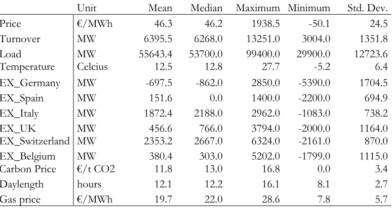
Table 1. Descriptive Statistics
Unit Mean Median Maximum Minimum Std. Dev.
Price €/MWh 46.3 46.2 1938.5 -50.1 24.5
Turnover MW 6395.5 6268.0 13251.0 3004.0 1351.8
Load MW 55643.4 53700.0 99400.0 29900.0 12723.6
Temperature Celcius 12.5 12.8 27.7 -5.2 6.4
EX_Germany MW -697.5 -862.0 2850.0 -5390.0 1704.5
EX_Spain MW 151.6 0.0 1400.0 -2200.0 694.9
EX_Italy MW 1872.4 2188.0 2962.0 -1083.0 738.2
EX_UK MW 456.6 766.0 3794.0 -2000.0 1164.0
EX_Switzerland MW 2353.2 2667.0 6324.0 -2161.0 870.0
EX_Belgium MW 380.4 303.0 5202.0 -1799.0 1115.0
Carbon Price €/t CO2 11.8 13.0 16.8 0.0 3.4
Daylength hours 12.1 12.2 16.1 8.1 2.7
Gas price €/MWh 19.7 22.0 28.6 7.8 5.7
Sample period: January 1, 2008 to December 31, 2012. N=35 065 for price, turnover, load, volumes of exchange and temperature and N=1461 for gas and carbon price, daylength.
Table 1 gives summary statistics for sample variables. The power prices, turnover, load, volumes of exchange and temperature have hourly frequency while daylength, the gas price and the carbon price are available at a daily frequency. The whole sample spans from January 01, 2009 to December 31, 2012, yielding 1461 daily observations for each trading hour. Several unit root tests (Augmented Dickey-Fuller, Phillips Perron) are applied to each variable, all series are found stationary at the usual significance levels except for gas price (the results are available upon request). In the following, we are considering gas prices in difference.
We rewrite equations (10) and (12) by substituting in for and from (11) and (13) to obtain:
Demand Function:
(14)
where is vector of all independent variables in the demand equation and is vector of parameters associated with .
Supply Equation:
(15)
where is vector of all independent variables in the supply relation and is vector of parameters associated with .
Qand lagged P) and and components. This is an issue raised uniquely in the
dynamic panel data models. It is because is a function of or in equations (14) and (15), it immediately follows that is also a function of or (because these components are time-invariant). Therefore, , a right-hand regressor in (14) and (15), is correlated with the error term, which renders the estimators biased and inconsistent even if the and are not serially correlated (Baltagi[2008]). There are broadly two methods to overcome this problem by wiping out the individual effects and .
Arellano and Bond [1991] proposed a transformation by first differencing to eliminate the individual effects and using the matrix of instruments where is given by:
[
]
The Arellano and Bond method is appealing because it uses the instrument set of lagged values of dependent variables, thus requiring no external instrumental variables. However, this method is uniquely appropriate to a micro panel dataset with and T very small. When , the matrix of instruments would become quickly unmanageable. With T=1461 as in our case, the number of instruments would be exploded, even if we break the whole datasat into several sub-sample.
The second choice to deal with the problem of introducing lagged dependent variable is to include the fixed effects (FE) estimator (Winthin transformation) in order to wipe out the individual effects and . Nickell [1981] shows that the dynamic panel models with fixed effects are biased of (1/T). However, as , the fixed effects estimator becomes consistent because the bias will not be large. Therefore, in the following we are considering the fixed effects dynamic panel model. Given that T=1461, the bias could be as small as 0.00069=1/1461 of the true value of the coefficients.
Furthermore, the fixed effects models seems to be a more appropriate specification for our dataset with individual dimension N (hours) is relatively small. Thus, it would not lead to a loss of degrees of freedom. We justify this choice by Hausman specification test (Hausman [1978]), which assumes random effects (RE) estimator to be fully efficient under null hypothesis. The results of the Hausman test give the overall statistics, χ2(7) for demand equation and χ2(13) for supply relation,
having p-value=0.000. This leads to strong rejection of the null hypothesis that RE provides consistent estimates. We are considering therefore the fixed effects model in both demand and supply functions.
Miller, Cameron and Gelbach [2009] and Thompson [2011], are used to assure that the estimators are consistent to arbitrary within-panel autocorrelation and contemporaneous cross-panel correlation.
6. EMPIRICAL RESULTS
6.1 Demand Function
The two-stage generalized method of moments (GMM) was employed to estimate the demand function (10). To control for endogeneity in
the matrix of excluded variables including lagged (1) values of carbon prices, gas prices and exchange balances with neighboring markets as well as lag-1; lag-7 of power price and forecasted load are used as instruments. The results of the first stage are convincing with is at 0.82 and very high F-statistics (197.66).
In order to choose the number of lags for autoregressive distributed lag terms, we start with k=7 then test our models down by excluding non-significant lags. The results suggest that only the lag-1 of the turnovers Q is kept. The long term elasticity of demand ( ) is then calculated using equation (9).
The second stage GMM estimation results for the demand function with panel dataset are reported in table 2. The parameter estimates are highly significant and with expected signs.
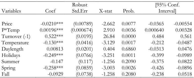
Table 2. Panel data model – Demand Equation
Variables Coef Robust Std.Err X-stat Prob. [95% Conf. Interval]
Price -0.0210*** (0.00789) -2.662 0.0077 -0.0365 -0.00554 P*Temp 0.00196*** (0.000674) 2.910 0.0036 0.000640 0.00328 Turnover (-1) 0.522*** (0.0195) 26.84 0.0000 0.484 0.561 Temperature -0.130*** (0.0416) -3.129 0.0017 -0.212 -0.0487 Daylength 0.00813 (0.0201) 0.404 0.6860 -0.0313 0.0476 Holidays -0.249*** (0.0766) -3.251 0.0011 -0.399 -0.0989
Summer -0.147 (0.117) -1.256 0.2090 -0.375 0.0822
Spring -0.258*** (0.0859) -3.003 0.0026 -0.426 -0.0896
Fall -0.0929 (0.0738) -1.258 0.2080 -0.238 0.0518
*** p<0.01, ** p<0.05, * p<0.1 . Robust standard errors in parentheses
and fall as electricity demand is supposed to be higher on average in winter. The coefficient of interacted term Price*Temperature is significant and positive at 0.002.
We use generated form (8) as an endogenous regressor in the supply relationship to reveal the existence of market power.
6.2 Supply Relation
We arbitrarily choose the quadratic form for the supply function with respect to "forecasted load". The excluded variables temperature, daylength are used as instruments to identify the supply functions. We include seven autoregressive terms AR(1-7).
The second stage GMM estimation results for the supply relations with panel dataset are reported in table 3. The parameter estimates are also generally significant and with expected signs except for gas and carbon prices.
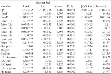
Table 3. Panel data model - Supply Equation
Variable Coef Robust Std. Err Z-stat Prob. [95% Conf. Interval] Q* 1.33e-05* -7.46E-06 1.787 0.0871 -2.10E-06 2.88E-05
Load 0.346*** -0.051 6.797 0.0000 0.241 0.452
Load² 0.00130*** -0.000309 4.192 0.0003 0.000657 0.00194 Price (-1) 0.276*** -0.0287 9.623 0.0000 0.216 0.335 Price (-2) 0.0783*** -0.0155 5.066 0.0000 0.0463 0.11 Price (-3) 0.0603*** -0.00987 6.106 0.0000 0.0399 0.0807 Price (-4) 0.0533*** -0.0082 6.498 0.0000 0.0363 0.0703 Price (-5) 0.00692 -0.0106 0.652 0.5210 -0.015 0.0289 Price (-6) 0.0350*** -0.00999 3.5 0.0019 0.0143 0.0556 Price (-7) 0.115*** -0.0202 5.683 0.0000 0.0732 0.157
Gas price 0.142 -0.116 1.226 0.2330 -0.0974 0.381
Margin -0.629*** -0.0569 -11.05 0.0000 -0.747 -0.511
Carbon -0.0241 -0.0191 -1.259 0.2210 -0.0636 0.0155
EX Germany 0.180*** -0.0625 2.879 0.0085 0.0507 0.309 EX Italy -1.887*** -0.302 -6.239 0.0000 -2.513 -1.261 EX Spain -0.960*** -0.233 -4.123 0.0004 -1.442 -0.478 EX Belgium 0.278*** -0.0814 3.409 0.0024 0.109 0.446 Holidays -6.935*** -1.546 -4.486 0.0002 -10.13 -3.737 *** p<0.01, ** p<0.05, * p<0.1. Robust standard errors in parentheses
The insignificance of estimated coefficient of gas price can be explained by the fact that the share of gas generation technology accounts for a very small part in the total annual marginality duration in France. The impact of marginality of gas plants on electricity prices in France is captured mostly through exchanges with neighboring countries like the UK, Italy or Belgium where gas represents a large share in the technology mix. Furthermore, due to the high gas price and relatively
10 The insignificance of seasonal dummies (summer and fall) can be explained by the fact that
low coal price in Europe, many of gas plants have been shutdown, which partly explains the non-significance of gas price's coefficient.
The coefficient estimate for carbon price is also showed insignificant. Indeed, we are studying the period of 2009-2012, where CO2 market was at the second phase and carbon price had significantly driven down to the absurdly low level, at around 2.5€/ton of CO2 at the end of period. Thus the relationship between CO2 price and electricity price seems to be not evident during the examined period, as also found in Jouvet and Solier [2013].
Finally and most importantly, the coefficient associated to Q* is significantly only at 10 %, and is very close to zero (1.33.e-05) suggesting that on average we find no market power in the electricity market in France during the examined period.
6.3 Robustness Tests
We conduct the robustness test by employing the model for each hour of the day.
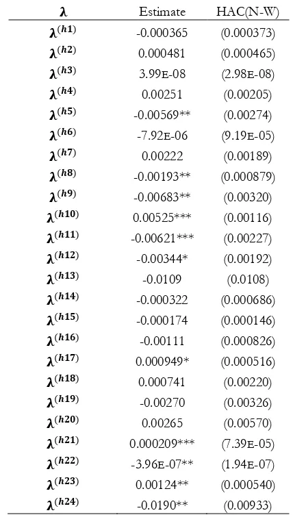
Table 4. Estimates for the market power parameters across hours
Estimate HAC(N-W)
( ) -0.000365 (0.000373) ( ) 0.000481 (0.000465) ( ) 3.99E-08 (2.98E-08) ( ) 0.00251 (0.00205) ( ) -0.00569** (0.00274) ( ) -7.92E-06 (9.19E-05) ( ) 0.00222 (0.00189) ( ) -0.00193** (0.000879) ( ) -0.00683** (0.00320)
( ) 0.00525*** (0.00116)
( ) -0.00621*** (0.00227)
( ) -0.00344* (0.00192)
( ) -0.0109 (0.0108)
( ) -0.000322 (0.000686)
( ) -0.000174 (0.000146)
( ) -0.00111 (0.000826)
( ) 0.000949* (0.000516)
( ) 0.000741 (0.00220)
( ) -0.00270 (0.00326)
( ) 0.00265 (0.00570)
( ) 0.000209*** (7.39E-05)
( ) -3.96E-07** (1.94E-07)
( ) 0.00124** (0.000540)
( ) -0.0190** (0.00933)
Standard errors (HAC Newey-West) are in parentheses
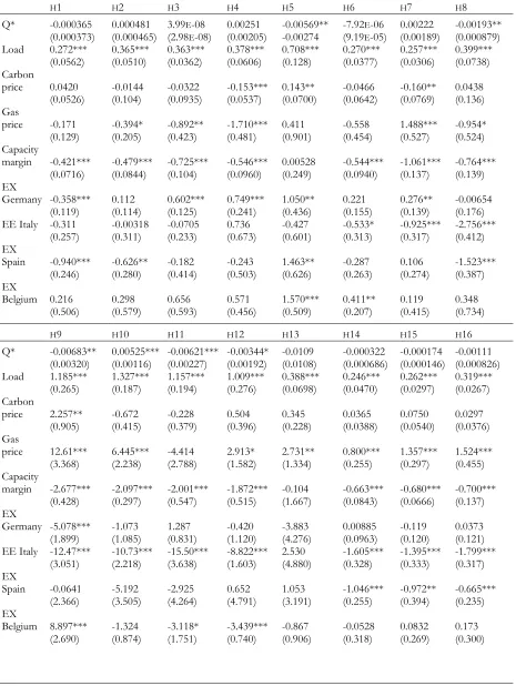
The second stage GMM results for both demand and supply equations are reported in tables (6) and (7) in the Appendix. Table (4) presents estimates for the market power parameters ( )across hours of the day. They are found either statistically insignificant or positively significant at the usual levels except for several peak hours 5, 8, 9, 11, 12, 22 and 24, which are negatively significant. However, the estimates for those hours stay at relatively low level.
Price cost margins can be estimated for the hours with negative coefficients11, the
results are given in table 5. The very low levels of Lerner indexes suggest that no market power has been exercised over the sample period.
Table 5. Lerner index across hours
LI-h5 LI-h8 LI-h9 LI-h11 LI-h22
Short term 0.01963641 0.02803341 0.04188475 0.01715386 4.7438E-07 Long term 0.0446282 0.03467772 0.02644286 0.01000519 8.7443E-07
6.4 Discussion
Despites of some doubts arose about the performance of wholesale electricity market in France, the model-based result suggesting the non-existence of market power is not really surprising. In fact, there are several economic arguments to justify this finding.
The total volume of electricity traded in wholesale market, though increasing since 2005, represents as small as 17% of the total electricity produced and sold in France. More importantly, the wholesale market is extremely regulated with the co-existence of market price and regulated tariff (ARENH price in wholesale market). The ARENH price was set by the French government at 42 €/MWh, which is relatively high. During the examined period, the frequency of spot prices observed in the wholesale market to be lower than 42 €/MWh is up to 40%. The alternative suppliers might sometimes prefer to buy electricity at the spot prices rather than regulated tariff. To make the long story short, as long as "market" comprises about only 17% of domestic delivery, the market integration with neighboring markets is increasingly strengthened, and prices in the spot market stay strictly regulated, it is extremely hard for an incumbent to exercise its market power even if it possesses one.
After all, Electricité de France (EDF), the incumbent in France and also the biggest producer of electric power in Europe, does not have economic incentives to exercise its market power because the possible gains from doing this would fall far behind the risks of being broken up the monopoly by the competition authorities. The high prices observed in French spot market since 2005 could be possibly explained by a number of exogenous reasons but hardly by market power abuse. Indeed, the trend of increased electricity price has been common in many power markets in Europe in the last decade because of many dramatic changes: the
11 Price-cost margin
( )
⁄ . The Lerner's measure is: ( )
implication of carbon price since 2005, the global economic crisis in 2008 pushing up the fuel costs to the highest level in the history, the catastrophe of Fukushima in Japan in 2011 adding burden to the costs of nuclear technology, the continuous political turbulence in Arabs countries followed by the increase of fuel prices, etc.
The doubts provoked on French spot prices due to the growingly divergence with German spot prices could be justified by the increasing share of renewable power generation in the German electricity portfolio. In fact, the next day of Fukushima nuclear accident, the German government decided to accelerate the phase-out of nuclear fleet by 2022, starting with the immediate closure of the eight oldest nuclear plants. Although fossil fuels fired energy has to put in place during the transitional period, renewable electricity generation is being considered as cornerstone of current and future energy supply. In Germany, a lot of support scheme for the development of renewable electricity generation have been put in place. Over the last ten years, the installed wind turbine capacity in Germany has increased with a factor of 5, from 6 GW in 2000 to 31,3 GW in 2012, and that of photovoltaic has raised from only 100 MW in 2000 up to 32,6 GW in 2012. The massive integration of renewable into electricity system creates a reduction effect (or merit-order effect) on German spot prices because this type of energy is bided zero in the merit order. This would be the reason why price divergence between France and Germany has been increasing despite a strong interconnected network.
7. CONCLUSION
The ongoing reorganization of the French electricity market will lead to an increasing volume of trade on the wholesale market. This being the case, developing relevant market power detection tools for electricity spot markets is a key issue for both academics and regulators.
In this paper we employ a structural model developed in New Empirical Industrial Organization (NEIO) to investigate the presence of market power abuse in the French wholesale electricity market during a panel data framework for hourly data during 2009-2012. The model-based results suggest that on average, no market power has been exercised during the examined period. Although market power is found statistically significant in several peak-load hours, it stays at very low level. There are many economic justifications to support this conclusion. Indeed, market power will hardly be abused if the "market" itself is extremely regulated as the case in France. Indeed, the price of electricity in France is lower than the average level of Europe. This difference reflects less and less the advantage from the "nuclear choice" made in the past, but more and more a good will to protect consumers from the tensions of actual energy world. Although no market power is exercised, the price system in France with the overlap of different prices and regulated tariff seems now to become too far to be able to send the right signals to investors and consumers.
important revolution of the electric power markets in France which is about to be significantly more liquid within a year, the market level estimated under different scenario of development would also be worth estimating.
REFERENCES
Arellano, M., & Bond, S. (1991). Some tests of specification for panel data: Monte Carlo evidence and an application to employment equations.The review of economic studies,58(2), 277-297.
Arellano, M. S. (2003). Diagnosing and mitigating market power in Chile's electricity industry.
Baltagi, B. (2008).Econometric analysis of panel data(Vol. 1). John Wiley & Sons.
Bask, M., Lundgren, J., & Rudholm, N. (2011). Market power in the expanding Nordic power market.Applied Economics,43(9), 1035-1043.
Bordignon, S., Bunn, D. W., Lisi, F., & Nan, F. (2013). Combining day-ahead forecasts for British electricity prices.Energy Economics,35, 88-103.
Borenstein, S. (2000). Understanding competitive pricing and market power in wholesale electricity markets.The Electricity Journal,13(6), 49-57.
Borenstein, S., & Bushnell, J. (1999). An empirical analysis of the potential for market power in California’s electricity industry.The Journal of Industrial Economics,47(3), 285-323.
Borenstein, S., Bushnell, J., & Wolak, F. (2000).Diagnosing market power in California's restructured wholesale electricity market(No. w7868). National Bureau of Economic Research.
Bresnahan, T. F. (1982). The oligopoly solution concept is identified.Economics Letters,10(1), 87-92.
Bushnell, J., & Saravia, C. (2002). An empirical assessment of the competitiveness of the New England electricity market.
Champsaur, P, Percebois J, and Durieux B. (2011) Rapport de la commission sur le prix de l'accès régulé à l'électricité nucléaire historique (ARENH), Le ministère de l'Écologie, du Développement durable et de l' Energie.
Competition (2007), Directorate-General, DG Competition report on energy sector inquiry, SEC (2006), 2007, 1724.
Conejo, A. J., Contreras, J., Espinola, R., & Plazas, M. A. (2005). Forecasting electricity prices for a day-ahead pool-based electric energy market.International Journal of Forecasting,21(3), 435-462.
Escribano, A., Ignacio Peña, J., & Villaplana, P. (2011). Modelling Electricity Prices: International Evidence*.Oxford bulletin of economics and statistics,73(5), 622-650.
Green, R. J. (2004). Did English generators play Cournot? Capacity withholding in the electricity pool.
Green, R. J., & Newbery, D. M. (1992). Competition in the British electricity spot market.Journal of political economy, 929-953.
Halseth, A. (1999). Market power in the Nordic electricity market.Utilities Policy,7(4), 259-268.
Hausman, J. A. (1978). Specification tests in econometrics.Econometrica: Journal of the Econometric Society, 1251-1271.
Hjalmarsson, E. (2000). Nord Pool: A power market without market power.rapport nr.: Working Papers in Economics, (28).
Huisman, R., Huurman, C., & Mahieu, R. (2007). Hourly electricity prices in day-ahead markets.Energy Economics,29(2), 240-248.
Jouvet, P. A., & Solier, B. (2013). An overview of CO2 cost pass-through to electricity prices in Europe.Energy Policy,61, 1370-1376.
Karakatsani, N. V., & Bunn, D. W. (2008). Forecasting electricity prices: The impact of fundamentals and time-varying coefficients.International Journal of Forecasting,24(4), 764-785.
Koopman, S. J., Ooms, M., & Carnero, M. A. (2007). Periodic seasonal reg-arfima–garch models for daily electricity spot prices.Journal of the American Statistical Association,102(477), 16-27.
Lang, C. (2006). Rise in German Wholesale Electricity Prices: Fundamental Factors, Exercise of Market Power, or Both?.Exercise of Market Power, or Both.
Lau, L. J. (1982). On identifying the degree of competitiveness from industry price and output data.Economics Letters,10(1), 93-99.
Liu, H., & Shi, J. (2013). Applying ARMA–GARCH approaches to forecasting short-term electricity prices.Energy Economics,37, 152-166.
Meritet, S. (2007). French perspectives in the emerging European Union energy policy.Energy Policy,35(10), 4767-4771.
Miller, D. L., Cameron, A. C., & Gelbach, J. (2009).Robust inference with multi-way clustering(No. 09, 9). Working Papers, University of California, Department of Economics.
Möst, D., & Genoese, M. (2009). Market power in the German wholesale electricity market.The Journal of Energy Markets,2(2), 47-74.
Müsgens, F. (2006). Quantifying market power in the German wholesale electricity market using a dynamic multi-regional dispatch model, The Journal of Industrial Economics, 54 (4), 471-498.
Nickell, S. (1981). Biases in dynamic models with fixed effects.Econometrica: Journal of the Econometric Society, 1417-1426.
Nogales, F. J., Contreras, J., Conejo, A. J., & Espínola, R. (2002). Forecasting next-day electricity prices by time series models.Power Systems, IEEE Transactions on,17(2), 342-348.
Schlueter, S. (2010). A long-term/short-term model for daily electricity prices with dynamic volatility.Energy Economics,32(5), 1074-1081.
Sheffrin, A. (2002, December). Predicting market power using the residual supply index. InFERC Market Monitoring Workshop December(pp. 3-4).
Steen, F. (2003). Do bottlenecks generate market power?: An empirical study of the Norwegian electricity market, Norwegian School of Economics and Business Administration. Department of Economics.
Steen, F., & Salvanes, K. G. (1999). Testing for market power using a dynamic oligopoly model.International Journal of Industrial Organization,17(2), 147-177.
Thompson, S. B. (2011). Simple formulas for standard errors that cluster by both firm and time.Journal of Financial Economics,99(1), 1-10.
Twomey, P., Green, R. J., Neuhoff, K., & Newbery, D. (2006). A review of the monitoring of market power the possible roles of tsos in monitoring for market power issues in congested transmission systems.
Weigt, H., & Hirschhausen, C. V. (2008). Price formation and market power in the German wholesale electricity market in 2006.Energy policy,36(11), 4227-4234.
Weron, R., & Misiorek, A. (2008). Forecasting spot electricity prices: A comparison of parametric and semiparametric time series models.International Journal of Forecasting,24(4), 744-763.
Price Temperature P*Temp Daylength Turnover(-1)
h1 -0.0246*** (0.00481) -0.143*** (0.0206) 0.00266*** (0.000438) 0.00884 (0.00965) 0.531*** (0.00452) h2 -0.0251*** (0.00336) -0.135*** (0.0139) 0.00271*** (0.000290) 0.0170* (0.00920) 0.514*** (0.00567) h3 -0.0296*** (0.00261) -0.129*** (0.00975) 0.00320*** (0.000227) 0.0261*** (0.00700) 0.534*** (0.00532) h4 -0.0529*** (0.00384) -0.153*** (0.0138) 0.00526*** (0.000330) 0.0220** (0.0103) 0.536*** (0.00704) h5 -0.0736*** (0.00414) -0.195*** (0.0153) 0.00708*** (0.000385) 0.0279** (0.0111) 0.550*** (0.00643) h6 -0.0574*** (0.00407) -0.206*** (0.0147) 0.00584*** (0.000352) 0.0563*** (0.00939) 0.550*** (0.00857) h7 -0.0371*** (0.00440) -0.211*** (0.0185) 0.00476*** (0.000368) 0.0445*** (0.00945) 0.494*** (0.00711) h8 -0.00912*** (0.00197) -0.117*** (0.0122) 0.00185*** (0.000196) -0.000641 (0.0104) 0.488*** (0.00838) h9 -0.0207*** (0.00265) -0.128*** (0.0201) 0.00202*** (0.000305) -0.0312** (0.0151) 0.426*** (0.0111) h10 -0.0198*** (0.00309) -0.139*** (0.0345) 0.00157*** (0.000514) -0.0110 (0.0119) 0.000439*** (1.02e-05) h11 -0.0227*** (0.00407) -0.120*** (0.0338) 0.00114** (0.000510) 0.00589 (0.0115) 0.455*** (0.00725) h12 -0.0372*** (0.00492) -0.180*** (0.0306) 0.00206*** (0.000466) 0.0221* (0.0115) 0.458*** (0.00739) h13 -0.0468*** (0.00443) -0.262*** (0.0275) 0.00376*** (0.000404) 0.0104 (0.0136) 0.438*** (0.00581) h14 -0.0359*** (0.00494) -0.140*** (0.0244) 0.00198*** (0.000407) -0.0108 (0.0114) 0.452*** (0.00849) h15 -0.0280*** (0.00395) -0.0900*** (0.0201) 0.00129*** (0.000347) -0.0249** (0.0105) 0.471*** (0.00850) h16 -0.0404*** (0.00520) -0.130*** (0.0235) 0.00221*** (0.000436) -0.0702*** (0.0117) 0.492*** (0.00970) h17 -0.0369*** (0.00444) -0.119*** (0.0222) 0.00208*** (0.000394) -0.105*** (0.0123) 0.522*** (0.00812) h18 -0.0544*** (0.00749) -0.314*** (0.0341) 0.00537*** (0.000505) -0.0272 (0.0173) 0.489*** (0.0102) h19 -0.0287*** (0.00311) -0.308*** (0.0162) 0.00454*** (0.000213) 0.0750*** (0.0163) 0.415*** (0.00551) h20 -0.0490*** (0.00506) -0.377*** (0.0271) 0.00534*** (0.000359) 0.0936*** (0.0174) 0.412*** (0.00896) h21 -0.0718*** (0.00784) -0.489*** (0.0461) 0.00729*** (0.000690) 0.111*** (0.0194) 0.491*** (0.00888) h22 -0.109*** (0.00966) -0.603*** (0.0516) 0.0100*** (0.000823) 0.127*** (0.0249) 0.487*** (0.00838) h23 -0.0252*** (0.00339) -0.212*** (0.0168) 0.00338*** (0.000282) -0.0345*** (0.0111) 0.481*** (0.00603) h24 -0.00155 (0.0112) -0.0892 (0.0567) 0.00142 (0.00109) -0.0491** (0.0232) 0.493*** (0.0256)
Standard errors (HAC Newey-West) are in parentheses
H1 H2 H3 H4 H5 H6 H7 H8
Q* -0.000365 0.000481 3.99E-08 0.00251 -0.00569** -7.92E-06 0.00222 -0.00193** (0.000373) (0.000465) (2.98E-08) (0.00205) -0.00274 (9.19E-05) (0.00189) (0.000879) Load 0.272*** 0.365*** 0.363*** 0.378*** 0.708*** 0.270*** 0.257*** 0.399***
(0.0562) (0.0510) (0.0362) (0.0606) (0.128) (0.0377) (0.0306) (0.0738) Carbon
price 0.0420 -0.0144 -0.0322 -0.153*** 0.143** -0.0466 -0.160** 0.0438 (0.0526) (0.104) (0.0935) (0.0537) (0.0700) (0.0642) (0.0769) (0.136) Gas
price -0.171 -0.394* -0.892** -1.710*** 0.411 -0.558 1.488*** -0.954* (0.129) (0.205) (0.423) (0.481) (0.901) (0.454) (0.527) (0.524) Capacity
margin -0.421*** -0.479*** -0.725*** -0.546*** 0.00528 -0.544*** -1.061*** -0.764*** (0.0716) (0.0844) (0.104) (0.0960) (0.249) (0.0940) (0.137) (0.139) EX
Germany -0.358*** 0.112 0.602*** 0.749*** 1.050** 0.221 0.276** -0.00654 (0.119) (0.114) (0.125) (0.241) (0.436) (0.155) (0.139) (0.176) EE Italy -0.311 -0.00318 -0.0705 0.736 -0.427 -0.533* -0.925*** -2.756***
(0.257) (0.311) (0.233) (0.673) (0.601) (0.313) (0.317) (0.412) EX
Spain -0.940*** -0.626** -0.182 -0.243 1.463** -0.287 0.106 -1.523*** (0.246) (0.280) (0.414) (0.503) (0.626) (0.263) (0.274) (0.387) EX
Belgium 0.216 0.298 0.656 0.571 1.570*** 0.411** 0.119 0.348 (0.506) (0.579) (0.593) (0.456) (0.509) (0.207) (0.415) (0.734)
H9 H10 H11 H12 H13 H14 H15 H16
Q* -0.00683** 0.00525*** -0.00621*** -0.00344* -0.0109 -0.000322 -0.000174 -0.00111 (0.00320) (0.00116) (0.00227) (0.00192) (0.0108) (0.000686) (0.000146) (0.000826) Load 1.185*** 1.327*** 1.157*** 1.009*** 0.388*** 0.246*** 0.262*** 0.319***
(0.265) (0.187) (0.194) (0.276) (0.0698) (0.0470) (0.0297) (0.0267) Carbon
price 2.257** -0.672 -0.228 0.504 0.345 0.0365 0.0750 0.0297 (0.905) (0.415) (0.379) (0.396) (0.228) (0.0388) (0.0540) (0.0376) Gas
price 12.61*** 6.445*** -4.414 2.913* 2.731** 0.800*** 1.357*** 1.524*** (3.368) (2.238) (2.788) (1.582) (1.334) (0.255) (0.297) (0.455) Capacity
margin -2.677*** -2.097*** -2.001*** -1.872*** -0.104 -0.663*** -0.680*** -0.700*** (0.428) (0.297) (0.547) (0.515) (1.667) (0.0843) (0.0666) (0.137) EX
Germany -5.078*** -1.073 1.287 -0.420 -3.883 0.00885 -0.119 0.0373 (1.899) (1.085) (0.831) (1.120) (4.276) (0.0963) (0.120) (0.121) EE Italy -12.47*** -10.73*** -15.50*** -8.822*** 2.530 -1.605*** -1.395*** -1.799***
(3.051) (2.218) (3.638) (1.603) (4.880) (0.328) (0.333) (0.317) EX
Spain -0.0641 -5.192 -2.925 0.652 1.053 -1.046*** -0.972** -0.665*** (2.366) (3.505) (4.264) (4.791) (3.191) (0.255) (0.394) (0.235) EX
H17 H18 H19 H20 H21 H22 H23 H24 Q* 0.000949* 0.000741 -0.00270 0.00265 0.000209*** -3.96E-07** 0.00124** -0.0190**
(0.000516) (0.00220) (0.00326) (0.00570) (7.39E-05) (1.94E-07) (0.000540) (0.00933)
Load 0.282*** 0.371*** 0.560*** 0.475** 0.245*** 0.239*** 0.280*** 0.593*** (0.0384) (0.0340) (0.0759) (0.233) (0.0312) (0.0242) (0.0307) (0.206)
Carbon
price 0.0843*** 0.0278 -0.0459 -0.167 0.0709 0.0179 -0.139** -0.125 (0.0321) (0.0452) (0.0964) (0.150) (0.0514) (0.0574) (0.0561) (0.182)
Gas
price 1.405*** 1.018*** 1.698** 0.922** 0.0689 1.043*** 0.373 0.970 (0.302) (0.278) (0.693) (0.424) (0.146) (0.352) (0.366) (0.968)
Capacity
margin -0.599*** -0.613*** -0.943*** -0.776*** -0.667*** -0.395*** -0.238*** -0.244 (0.0481) (0.0527) (0.0838) (0.140) (0.137) (0.0791) (0.0681) (0.170)
EX
Germany -0.0667 0.104 0.362 0.486 -0.147 0.0527 0.0440 -0.158 (0.0805) (0.141) (0.419) (0.681) (0.111) (0.108) (0.120) (0.171)
EE Italy -1.453*** -1.830*** -3.132*** -1.539*** -0.864*** -1.104*** -0.382 2.066 (0.277) (0.310) (0.687) (0.420) (0.218) (0.250) (0.303) (1.523)
EX
Spain -1.288** -1.138*** -1.716*** -2.827*** -1.069** -1.979*** -1.204*** 1.392* (0.640) (0.364) (0.244) (0.457) (0.465) (0.248) (0.388) (0.830)
EX
Belgium 0.861*** 0.649*** 0.723 -0.513 1.077*** 0.662** -0.187 0.638 (0.244) (0.208) (0.630) (0.668) (0.345) (0.282) (0.216) (0.477)
Standard errors (HAC Newey-West) are in parentheses