Characterizing Coseismic Ionospheric Disturbance for Surface-Rupturing Earthquakes

(1)

FOR SURFACE-RUPTURING EARTHQUAKES

by

Rebekah Faith Lee

A thesis

submitted in partial fulfillment of the requirements for the degree of

Master of Science in Geophysics Boise State University

(2)

c 2017 Rebekah Faith Lee

(3)

DEFENSE COMMITTEE AND FINAL READING APPROVALS

of the thesis submitted by

Rebekah Faith Lee

Thesis Title: Characterizing Coseismic Ionospheric Disturbance for Surface-Rupturing Earthquakes

Date of Final Oral Examination: 25 October 2017

The following individuals read and discussed the dissertation submitted by student Rebekah Faith Lee, and they evaluated the student0s presentation and response to questions during the final oral examination. They found that the student passed the final oral examination.

Dylan Mikesell Ph.D. Chair, Supervisory Committee Jeffrey B. Johnson Ph.D. Member, Supervisory Committee Lee M. Liberty M.S. Member, Supervisory Committee

(4)

DEDICATION

To my parents. Who have always supported me in everything I do.

(5)

Thanks first and especially to my advisor, Dr. T. Dylan Mikesell for taking me on as one of your first students. I couldn’t have asked for a better advisor. Thank you for all your patient help throughout the past few years. Thanks also to Dr. Lucie M. Rolland for hosting me for two weeks in France to learn about extracting TEC and for all your continued help thereafter. Thanks to both Lucie and Dylan for the privilege to write a paper with you. Thanks to GSA for the research grants that made travel to France possible. Thanks to my committee for all your help. Thanks to Dr. Hunter A. Knox for introducing me to Dylan. Finally, thank you to everyone in the Geosciences department at Boise State University for providing such a collaborative and supportive work environment.

(6)

ABSTRACT

Coseismic ionospheric disturbances (CID) are commonly identified using global navi-gation space system (GNSS) satellites. Little research, however, has focused on using total electron content (TEC) observations to characterize acoustic sources on Earth’s surface. For this thesis, I investigate the applicability of an analytical method to invert the TEC for the acoustic wave. The inversion is based on the modeling of a transfer function. Deconvolving the TEC by the transfer function gives the acoustic wave. Inverting for the acoustic wave in this way would remove phase differences in the TEC created by atmospheric-ionospheric coupling. I test the assumption in the model of a 1D, vertically varying ionosphere by comparing numerical models of the TEC using 1D and 3D electron density divergences. I find the results are complex and recommend obtaining a transfer function that includes a 3D ionosphere. Regardless, even with the phase shift introduced by ionospheric coupling, we are able to apply seismic methods to the TEC.

I show an example of applying seismic methods to the TEC of the 2016 Kaikoura earthquake. In this chapter, I highlight the ionospheric response to the rupture. I use numerical modeling and find the TEC response to be more consistent with an acoustic source located northeast of the initial rupture. I also apply backprojection to the TEC for the first time and obtain a source just northwest of the rupture area. The errors in the backprojection are consistent with expected errors from local winds,

(7)

work, inversion of the acoustic wave should also improve backprojection results by removing phase differences in the TEC.

(8)

LIST OF FIGURES

1.1 The IPP is the intersection of the ionospheric height with the satellite-receiver line-of-site (LOS). . . 5 1.2 Figure from Heki et al.(2006) illustrating the three types of coseismic

signals in the ionosphere. The direct acoustic wave is generated by uplift around the epicenter (right side of figure). In the far field (left side of figure) Rayleigh waves generate acoustic waves similar to the first type but travel horizontally at the speed of the Rayleigh waves generating them. Finally, tsunamigenic earthquakes (center of figure) also excite internal gravity waves in the ionosphere. . . 5 1.3 Comparison of time series plots of vertical electron content (VEC) on

the day of the earthquake (right) and on the previous day (left). 1 VEC = 1014 _electrons/m2_{. These plots demonstrate signal that is consistent}

with the 4:31 am earthquake. The blue areas along the IPP tracks between 4.7 and 5.5 am on Jan 17 indicate higher amplitude VEC and are consistent with arrival times from numerical models. Figure from Calais & Minster (1995). . . 6

(13)

trubance propagating radially from the area near the epicenter (yel-low star). (b) Time series maps of the change to the TEC for az-imuths highlighted in insets, plotted in units of TECU = 1 ×101₆

electrons/m2_{. Gray solid and dashed lines represent slope of Rayleigh}

and direct-acoustic waves, respectively. Black rectangle indicates the characteristic N-wave. From Rolland et al. (2011) . . . 8 1.5 Example temperature profile (left) and corresponding velocity profile

(right) at ionospheric heights. Profile is for Van, Turkey on October 23, 2011. . . 10 1.6 Literature examples of modeling TEC. (a) Comparison of modeled

TEC (colored) with observed (gray) at near field for the 2011 Van, Turkey earthquake. Waveforms for stations in red show the character-istic N-wave. From Rolland et al. (2013). (b) Synthesized TEC from eight point sources for the 2004 Sumatra earthquake. Results for one station paired with two satellites are shown at the top (satellite 23) and bottom (satellite 13). Individual time series for each of the eight sections are at the bottom of each satellite-receiver. The combined syn-thetic (thick black line) and observed data are plotted directly above the individual time series. Amplitudes are relative as the synthesized signals have arbitrary scaling. From Hekiet al. (2006) . . . 12

(14)

2.1 Illustrations of modeling steps. (a) Example output from raytracing (left) of the travel times of the acoustic wave. Convolving the arrival times with a N-shaped source function produces a time series of the acoustic wave (right) at each point in space. (b) Electron density perturbation after coupling of the acoustic wave with the ionosphere 10 minutes after generation of the acoustic wave. The black line is the line-of-sight from the receiver (triangle) to the satellite. (c) Results from the integration along the line of sight over all times give the TEC time series in TEC units (TECU), where 1 TECU = 1016 el/m2. . . 19 2.2 Diagram of the relationship betweenL, K, r, andχ. The red triangle

is the ground receiver and * is the source location. . . 25

3.1 Station grid for the Van location. Other locations have grids with similar geometry. . . 28 3.2 Examples of the elevation angles for 2 satellites at the N Mid Lat

location. Elevation of angles of zero are when the satellite was below the horizon. . . 30 3.3 Waveform comparisons of 1D and 3D divergence results of modeled

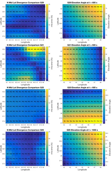
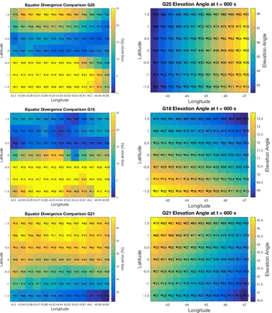
TEC. Stations are from the N Mid Lat grid and paired with the same satellite (G21). . . 31 3.4 Waveform differences and elevation angles for N Mid Lat grid location. 33 3.5 Waveform differences and elevation angles for N High Lat. . . 35 3.6 Waveform differences and elevation angles for Equator. Note change

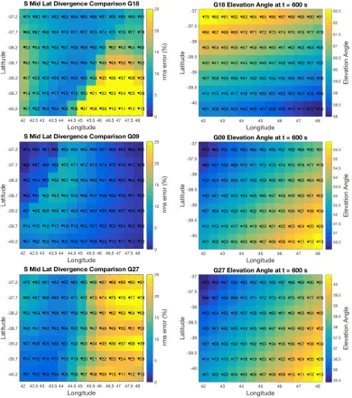
in the color axis in G21 to show higher errors. . . 36 3.7 Waveform differences and elevation angles for S Mid Lat. . . 37

(15)

3.9 Global background electron density on October 23, 2011 at 10:50am. 39

4.1 Workflow to extract TEC and convert to a MATLAB binary file. . . . 44 4.2 Example output from plot compact 2.m. The plot on the left shows

all satellites during a 24-hour time period. Satellites below the horizon have no data. The plot on the right displays times immediately before and after the 2011 Van (Turkey) earthquake. The black dashed line indicates the time of the earthquake. . . 45 4.3 Plots of TEC time series for GPS satellite number 21 and station

brmn (Turkey). Units are TEC units (TECU) where 1 TECU = 1016

electrons/m2_{. The parabola shape is due to the motion of the}

satel-lite as the line-of-sight length through the ionosphere changes as the satellite orbits the Earth. . . 46 4.4 Example of processing for a single TEC time series from the 2016

Kaikoura event. The raw data (top), TEC after polynomial detrend (middle), final TEC after filtering (bottom) . . . 48

5.1 Tectonic setting and major faults in New Zealand across the northeast part of the southern island. The large southern star marks the Kaik-oura earthquake epicenter estimated by USGS. The gray lines indicate plate boundaries, with other active faults as thin black lines. The star to the northeast of the southern island indicates the second location (Cape Campbell) where significant surface displacements occurred over a wide area (e.g. Hamling et al. (2017)). . . 54

(16)

5.2 Location of GNSS stations with IPP tracks for the six satellites for station WGTN (white triangle). Stars for each IPP track correspond to the earthquake onset time. Large star on south island is the initial rupture location. Rectangles are fault planes projected to the surface. 56 5.3 Left: Atmospheric sound speed profile computed from the NRLMSISE

model (Picone et al., 2002) on November 13, 2016 above the rupture area. Center: Atmospheric amplification factor. Right: Horizontal wind model computed from the NRLHWM (Drob et al., 2015) on the same day above Epicenter 1. . . 58 5.4 TEC observations from all stations plotted as a function of time and

epicentral distance. Distance is calculated from the IPP to two po-tential epicenters: (left) Epicenter 1 at 42.72◦S 173.06◦E and (middle) Epicenter 2 at 41.73◦S, 174.28◦. Grayscale (color online) indicates the amplitude of the TEC in TEC units (TECU), where 1 TECU = 1×1016

electrons per meter squared. The gray line marks the expected arrival time of an acoustic wave traveling radially at 1 km/s from the cho-sen epicenter and the x-intercept corresponds the time for the wave to propagate from the surface to an altitude of 320 km. Right: signal-to-noise ratio of observed (x and dots) and modeled (squares and tri-angles) TEC plotted by epicentral distance of the IPP at the time of maximum value of observed TEC for Epicenter 1 and Epicenter 2. . . 61 5.5 Stations with maximum amplitude≥0.05 TECU from those in Figure

5.4 for Epicenter 1 (left) and Epicenter 2 (middle). Right: SNR as in Figure 5.4 for selected stations . . . 63

(17)

IPPs trajectories at 320 km height for LOS linking GNSS stations marked as triangles to satellites G20 (northeast to south east tracks) and R22 (southwest to northeast tracks). The same time window as in Figure 5.2 is used. Additionally, the small stars mark the IPP locations at the earthquake onset time. The disks show the location of IPP when the observed TEC perturbation is maximum. Note that due to the GNSS satellites orbital motion, the IPP trajectories of satellite G20 (respectively R22) here describe a southwestward (respectively southward) translation of the selected network, moving southeastward (respectively northward) with time. The large stars mark the epicenter locations chosen as inputs to models 1 and 2. . . 64 5.7 Comparison of observed TEC time series (black, thick line) and

mod-eled TEC using Epicenter 1 (light, thin line) and Epicenter 2 (medium dark line). Time is in reference to the initialization of the Kaikoura rupture and correspondence to time zero for Model 1. Model 2 is shifted 60 seconds to account for the difference in start time. Maxi-mum observed TEC is shown at right, along with the distance from each epicenter to the station and the azimuth of the IPP at the time of maximum TEC. We indicate the maximum TEC time by a black dot for each observed TEC series. Stations are plotted in order of distance to the Epicenter 2 (medium dark line). The scale for the y-axis of each station is shown on the top stations. . . 65

(18)

5.8 Backprojection results from TEC synthetic time series for the Epicen-ter 1 model (large star). Most station and IPP locations lie to the northeast of the epicenter and have varying IPP tracks (e.g. station WGTN in Figure 5.2). . . 67 5.9 Backprojection results from observed TEC time series. The geographic

grid used here is 0.5×0.5 degrees. . . 68

5.10 Averaged backprojection results from satellites G20, R22 and G29 in Figure 5.9. The geographic grid used here is 0.1×0.1 degrees. . . 68

A.1 Comparison of 1D and 3D TEC results. (Left panel) Raw waveforms and RMS error for stations near Van, Turkey paired with satellite 21. (Right Panel) Amplitude normalized envelope of the raw waveforms and corresponding RMS error. . . 87 A.2 Same as A.1 but for satellite 30. . . 88

B.1 Interpolated TEC and best fit line to the maximum amplitude TEC. 90

C.1 Waveform differences and elevation angles for satellite G30 at N Mid Lat location. . . 92 C.2 Waveform differences and elevation angles for magnetic Equator.

Lat-itude: 7.58◦Declination: 0.39◦, Inclination 0.32◦ . . . 93

D.1 TEC time series data for Satellite R22. Stations below the cutoff of 0.05 TECU have been removed. . . 96 D.2 TEC time series data for Satellite R21. Stations below the cutoff of

0.05 TECU have been removed. . . 96

(19)

0.05 TECU have been removed. . . 97 D.4 TEC time series data for Satellite G05. Stations below the cutoff of

0.05 TECU have been removed. . . 97 D.5 TEC time series data for Satellite G13. Stations below the cutoff of

0.05 TECU have been removed. . . 98 D.6 Left: TEC waveform comparison for Satellite 21. Right: Map of IPP

locations from the time of the initial rupture to 35 minutes after. Epi-centers 1 and 2 are large stars and triangles are the stations on the ground. . . 98 D.7 Left: TEC waveform comparison for Satellite 29. Right: Map of IPP

locations from the time of the initial rupture to 35 minutes after. Epi-centers 1 and 2 are large stars and triangles are the stations on the ground. . . 101

(20)

LIST OF TABLES

1.1 TID sources and their contribution to TEC. . . 4

3.1 Earth’s magnetic field at the 4 test locations. Longitude for all loca-tions is 43.5◦E. . . 29 3.2 Times and satellites used to model the TEC at each test location. . . 30

(21)

CHAPTER 1:

INTRODUCTION & RESEARCH OBJECTIVE

1.1 Background

1.1.1 The Ionosphere

The ionosphere impacts modern society in several important ways. Because of the reflective nature of the upper ionosphere, we can send radio and communication trans-missions over great distances. Technology must also account for the ionosphere as disturbances in the ionosphere can interrupt signals from satellites. At high latitudes, the auroras create currents that can reach up to a million amperes and induce currents in power lines and pipelines (University of Alaska Fairbanks Geophysical Institute, 2017). The ionosphere also contains information of what happens in the Earth’s geospheres, and therefore is a means of remotely sensing processes occurring at the surface of the hydrosphere, the lithosphere and the atmosphere or ionosphere itself. Additionally, the ionosphere is the closest naturally occurring plasma, the most com-mon form of matter in the universe. Studying the ionosphere can help us understand this phase of matter.

(22)

2

region exists only during daylight and extends from about 50 km to 90 km and has low electron densities. The E region extends from 90–150 km and is more diffuse at night. Finally, the F region is divided into two layers, the F1 and F2 regions. During the night, the F1 layer decays creating a separation between the E and F2 layer. The majority of the electron density in the ionosphere falls within the F2 layer at about 300 km.

Disturbances to the ionosphere naturally occur at many different wavelengths from planetary to local scales. On a planetary level, Rossby waves result from variations with latitude of the strength of the Coriolis effect and have wavelengths thousands of kilometers long (Beer, 1974). At the medium and large scale, acoustic gravity waves propagate at tens to hundreds of meters per second with wavelengths of 100– 300 km for the medium scale and 300-3000 km for the large scale (Schunk & Nagy, 2000). Collectively, any disturbance propagating through the ionosphere is known as a traveling ionospheric disturbance (TID).

1.1.2 Total Electron Content

(23)

Galileo.

The interruption to GNSS by ionospheric disturbances is a result of the cumula-tive effects of the total electron content (TEC) along the satellite-receiver line of sight (LOS). GNSS automatically corrects these disruptions to the satellite signal by trans-mitting two frequencies. From these frequencies, the GNSS accounts for the TEC and returns travel times from the satellite to the receiver. Calais & Minster (1995) outline the method to obtain the TEC from GNSS data. The University Navstar Consor-tium (UNAVCO) also provides a software to obtain the TEC which is available online and which I use for this thesis (see Chapter 4). UNAVCO is a non-profit university-governed consortium that is funded through the National Science Foundation (NSF) and NASA.

Table 1.1 summarizes the impact of some common sources of TIDs on the TEC. The TEC perturbations are given either in TEC units (TECU), where 1 TECU = 1016 electrons/m2, or in percent change relative to the absolute TECU.

1.1.3 Ionospheric Pierce Point

(24)

4

Table 1.1: TID sources and their contribution to TEC.

Source TEC Perturbation Period Reference (min)

solar eclipses 0.15–15 TECU – Afraimovich et al. (2013) solar terminator 0.2–1 TECU 15 or 60 Afraimovich et al. (2013) solar flare ∼0.5 TECU 20–60 Afraimovich et al. (2013) tropical cyclone* _{2.5 TECU} _1–150 _Afraimovich _{et al.} ₍₂₀₁₃₎

rocket launches 0.2–2% 3–8 Afraimovich et al. (2013) geomagnetic storms 10–14 % – Afraimovich et al. (2013) earthquakes 1.8–6% 4–5 Astafyeva et al. (2014)

Heki et al. (2006) tsunami 0.15 8.7–14 Grawe & Makela (2015)

Occhipinti et al. (2013)

* _{TEC perturbation is at peak intensity. The effect disappears once winds}

are below 30 m/s.

the ionosphere off the coast, which demonstrates the utility of the TEC to sample over sources of subduction zone earthquakes in the ocean.

1.2 Identifying CIDs

A significant amount of research has demonstrated that coseismic ionospheric distur-bances (CIDs) can be identified in TEC signals obtained by GNSS (Calais & Minster, 1995; Artru et al., 2005; Afraimovich et al., 2010; Occhipinti et al., 2013; Astafyeva

et al., 2014). The literature identifies CIDs in two primary ways. Here I briefly describe these two methods and then show examples in the following section.

(25)

Figure 1.1: The IPP is the intersection of the ionospheric height with the satellite-receiver line-of-site (LOS).

(26)

6

Figure 1.3: Comparison of time series plots of vertical electron content (VEC) on the day of the earthquake (right) and on the previous day (left). 1 VEC = 1014 _electrons/m2_{. These plots demonstrate signal that is}

con-sistent with the 4:31 am earthquake. The blue areas along the IPP tracks between 4.7 and 5.5 am on Jan 17 indicate higher amplitude VEC and are consistent with arrival times from numerical models. Figure from Calais & Minster (1995).

signal is labeled in bold font and includes: (1) the direct acoustic wave from the uplift at the source (Heki & Ping, 2005; Afraimovichet al., 2010; Rollandet al., 2013; Occhipinti et al., 2013), (2) perturbations caused from Rayleigh waves traveling on the surface (Rolland et al., 2011; Occhipinti et al., 2013) and (3) internal gravity waves created by tsunamigenic earthquakes (Heki & Ping, 2005; Occhipinti et al., 2013). My research focuses on the direct acoustic wave signal. I discuss this class of CID for the remainder of this thesis. The second way researchers have confirmed the identity of CIDs is with numerical modeling of TEC response to CIDs (Heki et al., 2006; Rollandet al., 2011; Kheraniet al., 2012; Rollandet al., 2013), which has shown good agreement with observations. In the following sections I give some examples of identifying CIDs from the literature.

1.2.1 TEC Time Series

(27)

tech-nique. They observe fluctuations in electron content up to 1000 km (along the ground) from the January 17 1994, Mw6.7 Northridge (CA) earthquake. Figure 1.3 (right) shows a 3 hour time series window for January 16th and 17th. The IPP tracks are plotted as white dots and, through time, show a parabolic shape due to the motion of the satellite. The authors use the vertical electron content (VEC), which is the electron content summed vertically from a point in the ionosphere to the ground. The VEC is obtained from the TEC using basic trigonometry as VEC = h_LTEC, where h is the thickness of the ionosphere and L is the length of the ray path through the ionosphere. The January 17 plot (right) shows VEC with 1%−3% change in total electron content between the hours of 4:40 and 5:30 am local time at distances of about 100 km as well as between 220–450 km, which they note is consistent with previous observations after moderate-size earthquakes or nuclear explosions. Numer-ical simulations (Davies & Archambeau, 1996; Warshaw & Dubois, 1981) predict that the direct acoustic wave would arrive at ionospheric heights 10 to 15 minutes after ground displacement. The arrival times of the perturbations are therefore consistent with numerical simulations for the 4:31am (local time) earthquake. Figure 1.3 also shows the VEC for the previous day (left). No similar organized perturbation exists, further supporting the conclusion that the higher amplitudes in the VEC were cre-ated by an earthquake on the surface. The authors also compute the velocities of the first arrivals as 300 to 600 m/s. Because the velocity is in good agreement with numerical models of ionospheric acoustic-gravity waves generated by seismic sources, they interpret the source as the acoustic wave generated by uplift in the epicentral region.

(28)

rou-8

(a)

(b)

Figure 1.4: Example of typical CID presentations. (a) TEC Map shows the distrubance propagating radially from the area near the epicenter (yel-low star). (b) Time series maps of the change to the TEC for azimuths highlighted in insets, plotted in units of TECU = 1 ×101₆ _electrons/m2_.

(29)

tinely demonstrated through TEC maps in which the authors show the projection of the IPPs on the ground with a color map of the TEC amplitude, as well as through time series plots (see for example Heki & Ping (2005); Kherani et al.(2012); Occhip-inti et al. (2013); Grawe & Makela (2015); G˜omez et al. (2015)). Often the TEC is plotted as the change in the TEC by removing a polynomial fit of the TEC. This removes the influence of the moving satellite on the TEC.

(30)

10

Figure 1.5: Example temperature profile (left) and corresponding velocity profile (right) at ionospheric heights. Profile is for Van, Turkey on October 23, 2011.

Sound Speed

For perfect gases, sound travels at a velocity given by:

v2 =γp/ρ=γRT, (1.1)

whereγ is the ratio of specific heats (cp

cv), p is pressure,ρis the density of the air, R is the gas constant and T is the temperature (K). Therefore, the speed of sound is most influenced by temperature. Figure 1.5 shows an example profile of the temperature and resulting sound speed at different atmospheric heights. At the ionospheric height of 300 km, the temperature is 832◦ and the speed of sound is 900 m/s.

When the velocity of air particles becomes close to the speed of sound a ”shock-acoustic” effect occurs (Afraimovich et al., 2001) due to non-linear effects (Chum

(31)

1.4b shows an example of such a wave outlined by the rectangle and is also shown for individual waveforms in Figure 1.6a in red.

1.2.2 Modeling

A second method to support identification of a CID is to compare modeled output of a CID to observed data. Kherani et al. (2012) use finite differences to model tsunami-triggered acoustic gravity waves (AGWs) in the atmosphere as well as the ionospheric response. They find good agreement with observed data for the 2011 Tohoku-Oki tsunami.

Another method replaces finite difference calculations with acoustic ray tracing to model the acoustic wave, and is computationally less expensive (Heki & Ping, 2005; Dautermann et al., 2009; Rolland et al., 2013) . This method still employs finite differences in the propagation of the acoustic wave in the atmosphere and coupling with the ionosphere. This is the model I employ in this study. I describe the methods for the model in Chapter 2. Figure 1.6 shows two examples of this type of modeling from Rolland et al. (2011) and Heki et al. (2006) using single (1.6a) and multiple (1.6b) point sources, respectively.

Rolland et al.(2013) successfully model the TEC response to acoustic waves gen-erated by seismic sources. Figure 1.6a shows their model (colored), which agrees well with observed phase of the data (gray) from the 2011 Mω 7.1 Van earthquake.

(32)

12

(a) (b)

(33)

their model requires the use of a-posteriori information in order to assign relative am-plitudes to the eight acoustic waves generated at each segment. This second example of modeling TEC demonstrates the potential to recover source information from the TEC, specifically, the epicentral location on the surface as well as extent of rupture.

1.3 Source Information in TEC

Similar to the Heki et al.(2006) example, other research has begun to investigate the potential of TEC to recover earthquake source information. Some of the source infor-mation recovered includes earthquake location (Hekiet al., 2006; Liuet al., 2010), lat-eral rupture extent (Hekiet al., 2006), and slip mode (Rollandet al., 2013). Astafyeva & Heki (2009) suggest that the initial polarity of the TEC might be related to the initial motion of the coseismic neutral pressure wave. Rolland et al. (2013) test this hypothesis and demonstrate that the polarity is primarily linked to local geomagnetic field. It is worth noting however, in places where the geomagnetic field is parallel to the neutral disturbance, the initial polarity can reflect the direction of the first motion on the ground.

(34)

14

reaches a minimum that location is chosen as the hypocenter.

Finally, Rolland et al. (2013) show that the slip mode can also be inferred from TEC. They use a compressional point source consistent with a reverse fault rupture to model the TEC response to the 2011 Van earthquake (Turkey). The modeled data is in good agreement with observed data.

1.4 Significance

Because of the source information contained in the TEC, GNSS-TEC measurements play a potentially important role in earthquake and tsunami monitoring. The acous-tic wave, generated by earthquake displacement on the surface, travels to ionospheric heights within about 10 minutes. This creates the potential for near real-time charac-terization of surface uplift around the epicenter, whether on land or under the ocean, as the displacement on the ocean floor transfers directly to the water (Occhipinti

et al., 2013). While seismology offers useful tools to characterize the source, it is lim-ited by the proximity of seismic stations to the sources. TEC measurements offer a method to obtain data closer to the source, due to the ability to image the ionosphere along a line of sight that passes over water (see Figure 1.1). Moreover, the wave-field that propagates in the atmosphere is much less distorted than the wavewave-field that propagates in the Earth. This makes interpreting waveforms for source characteristics much simpler.

1.5 Research Objective

(35)

allows the application of tools from seismology to characterize the source phenomena. However, before we can successfully apply seismic techniques, we must take into account the physics of the CIDs traveling through the ionosphere. I will go into more detail on the physics of the wave propagation in the next chapter, but will highlight the main points here.

CIDs are created initially from acoustic (pressure) waves in the neutral atmosphere generated by vertical motion on the surface. The neutral atmospheric waves couple with the ionosphere in a complex way depending on the local geomagnetic field. There is also a change in the amplitude of the TEC response that depends on the geometry of the satellite and receiver. The situation is further complicated by the satellites’ motion. All of these factors need to be taken into account if we are to use the TEC to obtain source characteristics.

One method to do this is to invert for the acoustic wave and was first suggested by G˜omez et al. (2015). The TEC is equal to the acoustic wave times a transfer function in the frequency domain. To invert for the acoustic wave, they divide the observed TEC by the transfer function. To obtain the transfer function, they rely on an analytical model developed by Georges & Hooke (1970) (hereafter G&H analytical method). This method relies on two key assumptions: 1) a plane wave approximation of the propagating wave and 2) a 1D electron density divergence in the vertical direc-tion that is approximated by an analytical model of the ionosphere. They successfully apply this method to far-field (Antarctica) TEC signal produced by Rayleigh waves from the 2010 Maule and 2011 Tohoku-Oki earthquakes.

(36)

16

to the CID. The first part of this thesis investigates the applicability of the G&H analytical method to CID created by direct uplift around the epicenter. I examine one of the key assumptions that the electron density only varies significantly in the vertical direction. My research question for this part is: Under what (if any) conditions can we reliably assume a 1D ionosphere? I hypothesize that latitude as well as elevation angle of the satellite and geometry of the satellite-receiver line-of-sight may interact to create conditions that determine the applicability of the 1D ionosphere assumption. I expect that at lower elevation angles, the difference between a 1D and 3D ionosphere is greater due to the increased horizontal component of the line-of-sight.

To test this hypothesis, I use the spherical numerical model outlined by Rolland

et al. (2013) to examine the importance of a 3D ionosphere to the TEC. I describe both this numerical model and the G&H analytical method in the next chapter. I use the spherical numerical method to model the TEC using a 1D and 3D ionosphere at different latitudes and present the results in Chapter 3.

(37)

(38)

18

CHAPTER 2:

FORWARD MODELING TEC

2.1 Chapter Summary

I use the model outlined by Rollandet al.(2013) to investigate the influence of the 3D ionosphere on the TEC, and therefore the assumption of Georges & Hooke (1970) of a horizontally invarient ionosphere. In this chapter, I summarize the derivations of the TEC equations for both models in separate sections. Within each section, I describe the derivations in terms of three steps. These steps are illustrated in Figure 2.1 and described in greater detail in subsequent sections. They include: (1) generation and propagation of the acoustic wave, (2) electron density perturbations excited by the coupling of the acoustic wave with the ionosphere, and (3) integration of electron density perturbations along the line of site of the GNSS satellite-receiver pair.

2.2 Numerical Method

2.2.1 Acoustic Wave

(39)

(a)

(b) (c)

(40)

20

et al., 2005). An example of the output of the arrival times is shown on the left in Figure 2.1a. Note that each ray follows a curved path that is due to refraction of the acoustic wave by the atmosphere. Next, we convolve the ray amplitude with an N-wave source function (Heki & Ping, 2005; Dautermann et al., 2009) characteristic of the nonlinear effects of the propagation of the acoustic wave (see 1.2.1 or Chum

et al. (2016) for further explanation). This source function describes the atmospheric response to the piston-like motion of the ground at ground level:

u(t) = A √

2

σ3/2_π1/4(t−t0)e

−(t−t0)2

2σ2 , (2.1)

where A is the initial amplitude factor, t0 is the time of maximum displacement and

σ is the width of the pulse (Rolland et al., 2013). The model also accounts for the frequency-dependent viscous and thermal losses by scaling the pulse width so that it varies linearly as σ(t,r) = btarrival(r), where tarrival is the arrival time, and b is a scaling factor. The neutral wave particle velocity is then:

vn=uk. (2.2)

The result of the convolution produces a time series at all points in space. I show an example result on the right in Figure 2.1a.

2.2.2 Ionospheric Coupling

(41)

The neutral acoustic wave transfers its momentum directly to charged particles in the ionosphere. The velocity of the charged ions, vi, is equal to the component of

the neutral wave parallel with the geomagnetic field (Georges & Hooke, 1970):

vi = (vn·ˆb)bˆ=|vn||b|cosθ, (2.3)

where vn is the particle velocity of the neutral wave and bˆ is the geomagnetic

field direction. Equation (2.3) is commonly referred to as the ionospheric coupling factor (hereafter coupling factor), and is a fundamental description of atmosphere-ionosphere coupling.

I want to find the change in the electron density, ∂ne and so I use the continuity equation as the governing equation:

∂ne

∂t +∇ ·(ne0vi) = 0. (2.4)

where ne0 is the unperturbed electron density. In the remainder of this section I

ex-amine the 3D and 1D numerical solution to Equation 2.4 using a spherical wavefront. I address the analytical solution in Section 2.3.2. The analytical solution assumes a planar wave.

3D Divergence

Rolland et al. (2011) derive the 3D electron density, ∂ne, by solving the governing equation (Equation 2.4) using finite differences and integrating over time:

∂ne(r, t) =−

Z t

0

(42)

22

If we expand the integrand as:

∇ ·(ne0(vi)) =ne0(∇ ·vi) +vi· ∇ne0, (2.6)

we see that the perturbations in the electron density depend on both the divergence of the ionospheric wave and the gradient of the background electron density.

In spherical coordinates, Equation (2.6) is

∇ ·(ne0(vi)) = ne0 "

2

rvir+ ∂vir

∂r

+1 r

∂viθ ∂θ +

viθcosθ rsinθ

+ 1 rsinθ

∂viφ ∂φ

#

+vir ∂ηe0

∂r + viθ

r ∂ηe0

∂θ + viφ rsinθ

∂ηe0

∂φ . (2.7)

This 3D model serves as the baseline for analysis on this project. In order to analyze the applicability of the analytical model used by G˜omez et al. (2015), I also run the model using a simplified 1D divergence that is comparable to the analytic model.

1D Divergence

We can simplify Equation 2.7 to one dimension if we assume that only the partial derivative in the r direction is significant:

∇ ·(ne0(vi)) =ne0 "

2 rvir+

∂vir ∂r

#

+vir ∂ηe0

∂r . (2.8)

(43)

Equation (2.8) back into Equation ( 2.5) we obtain:

∂ne =−

Z t

0

ne0 "

2 rvir+

∂vir ∂r

#

+vir ∂ηe0

∂r dt. (2.9)

This represents a model where thene0 term varies only in the radial direction, as does

the plane wave in the analytical model.

2.2.3 Line of Sight Integration

The methods described in the previous section give the change in the electron density at any point in the ionosphere. In order to compare the 1D and 3D models with observed TEC we need to integrate along the line of site (LOS), L, of the receiver and GPS satellite so that:

T EC =

Z

LOS

∂ne dr. (2.10)

I show an example LOS and resulting TEC from integration in Figure 2.1b and 2.1c. I combine Equations ( 2.5) and ( 2.7) or (2.8) for the 3D or 1D cases, respectively. The 1D case is:

T EC =

Z

L

∂ne0(r,t)dr = Z L − " Z t 0

ne0 h2

rvir+ ∂vir

dr

i

+vir ∂ηe0

∂r dt

#

dr. (2.11)

(44)

24

2.3 Analytical Model

2.3.1 Acoustic Wave: Plane Wave Approximation

If our observation point is far enough away from the source we can assume a plane wave. Georges (1968) develops such an approach using a plane wave approximation of the neutral atmospheric wave:

vn(r, t, ω)≈V(z)ei(k·r−ωt),

where V(z) is the height dependent amplitude, ω is angular wave frequency, and

k is the wave vector with phase velocity c. The electron density perturbation in the ionosphere is similarly planar. During the atmosphere-ionosphere coupling, the phase of the acoustic wave is conserved; only the amplitude changes according to the coupling factor.

2.3.2 Ionospheric Coupling

Georges (1968) also assumes that the horizontal gradient of the background electron density is negligible and using the continuity equation (Equation 2.3) obtains a planar continuity equation:

∂ne(r, t) = 1 ω

vn(r,t)·bˆ

(k·bˆ)ne0(z) +i(ˆb·ˆz)

∂

∂zne0(z)

. (2.12)

.

(45)

*

IPP satellite ~k

ˆ

z

~

L

~r

Figure 2.2: Diagram of the relationship between L, K, r, and χ. The red triangle is the ground receiver and * is the source location.

2.3.3 Line of Sight Integration

Georges & Hooke (1970) derive the TEC by integrating Equation (2.12) along the LOS of the satellite-receiver pair. They obtain the following equation:

T EC = [uei(ωt+k·r)][ 1

ωcos2_(χ)][(ˆk·ˆb)(ˆr×ˆb)×ˆz·k][

Z ∞

−∞

ne0(hm+z0)e(iηz

0₎

dz0], (2.13) where: χ= cos(−1)_{(z/c) is the zenith angle of the LOS (}_L_{) and is shown in Figure}

(2.2), z0 = (z−hm), hm is the altitude of the peak electron density, and η= k_h_m·r. This equation still includes an integration term. The authors give several analyti-cal approximations of the ionospheric profile, including anα-chapman approximation, where the normalized background electron density is given by:

ne0

nem

=e2i(i−

z0 H−e

−z0/H₎

, (2.14)

(46)

26

Z ∞

−∞

ne0(hm+z0)e(iηz

0₎

dz0] = 2 −iηH √

π Γ( 1

2−iηH), (2.15)

where Γ is the gamma function of complex argument and H is the thickness of iono-sphere. Equation 2.13 then becomes

T EC = [uei(ωt+k·r)][ 1

ωcos(χ)2][(ˆk·bˆ)(ˆr×bˆ)×ˆz·k][

2−iηH √

π Γ( 1

2−iηH)] (2.16)

This is the final equation for the TEC using the Georges and Hooke model.

(47)

CHAPTER 3:

TEC SENSITIVITY TO MODEL PARAMETERS

3.1 Chapter Summary

In Chapter 2, I outlined the methods used to model the TEC developed in Rolland

et al. (2011). To move toward an analytical model such as that employed by G˜omez

(48)

28

Figure 3.1: Station grid for the Van location. Other locations have grids with similar geometry.

3.2 Methods

3.2.1 Station Grid

For each test location, I use a grid of stations that is 333 km north to south and 522 km east to west. Stations are separated by ∼43.5 km in the longitude direction and 55.5 km in the latitude direction. The epicenter is approximately in the middle latitude and one quarter the total distance in the longitude direction. This produces a grid that is 7 x 13 stations. Figure 3.1 shows the station layout for an epicenter location at the site of the 2011 Mw 7.1 Van earthquake (38.7◦N, 43.5◦E). This was the

(49)

Table 3.1: Earth’s magnetic field at the 4 test locations. Longitude for all locations is 43.5◦E.

Location Latitude (◦) Inclination (◦) Declination (◦) IPP height (km)

N High Lat 75 82 20 300

N Mid Lat 38.7 57 5 260

Equator 0 -18 -1 380

S Mid Lat -38.7 -62 -37 290

S High -75 -68 -57 260

idealized, station grid. Text beside each station gives station names.

3.2.2 Grid Locations

Earth’s magnetic field has an important impact on the TEC (Heki et al., 2006). Per-turbations from the acoustic wave couple to the ionosphere and transfer momentum into electrons parallel to the Earth’s magnetic field. I test this effect on the 1D diver-gence assumption by using the same grid at mid and high latitudes, and the Equator. I use the same longitude for all locations. For the mid latitude epicenters I use the 2011 Van earthquake location for the Northern Hemisphere (hereafter N Mid Lat) and -38.7 degrees for the southern latitude (S Mid Lat). For the high northern (N High Lat) and southern (S High Lat) latitudes I use±75 degrees, respectively. Table 3.1 shows the inclination and declination at each of these locations along with the IPP height used. For the IPP height, I use the maximum electron density height for each location.

3.2.3 Satellite Positions

(50)

30

Figure 3.2: Examples of the elevation angles for 2 satellites at the N Mid Lat location. Elevation of angles of zero are when the satellite was below the horizon.

with all satellites during the day of October 23, 2011. Examples of the elevation angles for 2 satellites at the N Mid Lat location are shown in Figure 3.2. For all but the N High Lat, I chose a time during daylight hours that is close to the time of the maximum elevation angle for 2-3 satellites. The N High Lat was in 24 hour darkness during this time. The times and satellites chosen are presented in Table 3.2.

Table 3.2: Times and satellites used to model the TEC at each test loca-tion.

Location Time (UTC) Satellites N High Lat 10:50 G5, G29 G30

(51)

3.3 Results

3.3.1 Impact of Electron Density Divergence on TEC

I show an example of the modeled TEC for 1D and 3D divergence for two stations in Figure 3.3. Both waveforms are for the N Mid Lat grid location for satellite 21 (G21, where G indicates a GPS constellation satellite for all satellites hereafter). Station 8 (top) is an example where the 1D divergence has significant phase differences, whereas station 25 (bottom) shows some amplitude difference but fits the phase. In Appendix A, I show analysis of the misfit that shows that energy is conserved between the 1D and 3D divergence, but that the phase varies significantly. See Figure 3.1 for station locations.

(52)

32

Figure 3.4 shows the elevation angles for all stations (right column) as well as the RMS (left column) for 4 of the 5 satellites in view at 10:50 am. Satellite numbers are given for each plot and are in order of decreasing elevation angles from top to bottom. For each satellite except G05, I found the elevation angle for all stations at time t= 600 seconds. This time corresponds with the arrival times in the modeled TEC time series. Satellite G05 had overall lower satellite angles during the minutes after the modeled event. The lower angles produce IPPs further from the stations and thus later arrival times. Therefore, I use a time consistent with arrival times for G05 of 1000 seconds to plot the elevation angle. Together, the four satellites cover a range of elevations from about 34 degrees up to a high of about 76 degrees (G29). Areas with the highest elevation angle in each plot indicate the direction that IPPs are shifted relative to the stations on the ground. Satellites G05 and G29 have IPPs to the northeast of the stations while G21 and G25 are shifted to the west and south, respectively.

The RMS differences for all satellites was low (see left column, Figure 3.4). Only satellite G21 showed an error above 15%. See station 8 in Figure 3.3 and 3.4 for an example of a high-error station contrasted with a station (25) with smaller waveform differences. The highest error was 32% and is in the north east corner. The fifth satellite in view, G30 (see appendix, Figure C.1) had similar elevation angles and RMS to G21.

3.3.2 Magnetic Field Influence on TEC

(53)

(54)

34

elevation angles), the N High Lat (see Figure 3.5) was the only other location with consistently low RMS differences, indicating that the vertical divergence is adequate for modeling purposes.

At the Equator (Figure 3.6), the two higher elevation satellites (G25 and G18) have some areas with lower error, while the low angle satellite (G21) shows the highest phase difference with over 60% difference in the RMS. Overall, the equator gave the highest RMS error of all locations.

At the S Mid Lat location (Figure 3.7), two satellites (G09 and G27) have IPPs to the southeast of the stations but with different elevation angles. Satellite G09 shows the lowest RMS error of the two and has higher elevation angles (50–55 vs. 35–40).

Results for the S High Lat (Figure 3.8) are also mixed. Satellites G09 and G27 have relatively low RMS error with areas of higher error. Both show a similar pattern in high error areas in the west part of the grid. The slight difference in the direction of the LOS (G27 to the east and G09 to the northeast) may account for the increased wave differences on the eastern side of the grid for G27.

(55)

(56)

36

(57)

(58)

38

(59)

Figure 3.9: Global background electron density on October 23, 2011 at 10:50am.

3.4 Discussion

The results from the modeling of the N Mid Lat location indicate that, in this case, a 1D approximation of the divergence is a reasonable assumption. Elevation angle had no apparent effect on the RMS differences. Results for the highest elevation angle (G29) were similar to those with the lowest (G05). The general direction from both these satellites was similar (to the northeast). Satellite G21 had the highest error and was the only satellite with LOS to the west of the stations. This suggests that the direction of the LOS is more important than elevation angle.

Results for the other test locations indicate low RMS error for both Northern Hemisphere locations (N High Lat and N Mid Lat). The higher error in G10 for the N High Lat indicates that very low elevation angles (less than 30◦ in this case) introduce error not present in any elevation above the cut-off elevation angle.

(60)

40

in the S Mid Lat location (Figure 3.7). A second satellite (G27), with similar LOS, but lower elevation angle has higher error. One interpretation of this result is that elevation angles have more influence in the Southern Hemisphere than in the Northern Hemisphere. However, the influence of the elevation angle is still secondary to the LOS as high elevation angles at the equator (G18 and G25 in Figure 3.6) do not yield lower error. The importance of a low cut off angle holds in both Northern and Southern Hemispheres. As with the N High Lat, elevation angles under 30◦ in the S High Lat produce more overall error (G18, Figure 3.8). For the Equator (the location with highest overall error) the cut-off for increased relative error is higher, with G21 showing markedly increased error under 45.5◦

Here I only observe the differences between the Northern and Southern Hemi-spheres. However, one explanation for the differences may be in the seasons. The tilt of the earth relative to the sun creates a difference in how direct the sun’s rays are in the Northern and Southern Hemispheres. During summer in the Northern Hemisphere, the Northern Hemisphere is tilted toward the sun whereas the Southern Hemisphere is titled away, because radiation from the sun is what strips electrons away from neutral atoms (thus creating the ionosphere), this difference in the seasons may be what is causing the 3D difference in the Southern Hemisphere in October.

(61)

3.5 Conclusion

For this thesis, I investigate the cause of the patterns in the RMS differences by exam-ining the elevation angles and receiver-satellite LOS as well as the global background electron density. While the LOS does impact the results, the relationship with the ionospheric structure is unclear. As discussed in Chapter 2, the coupling factor (Equa-tion 2.3) is a fundamental descrip(Equa-tion of atmospheric-ionospheric coupling. Therefore, a third plot of the projection of the acoustic wave onto the magnetic field could yield further insights.

These initial observations show that the reliability of the 1D assumption is com-plex. For an event in fall, the 1D assumption holds in the Northern Hemisphere. However, the direction of the LOS also plays a role and can introduce higher errors in small areas. Elevation angle has little impact on the results except at very low angles. This elevation angle cut off is higher at low latitudes near the Equator.

(62)

42

CHAPTER 4:

TEC EXTRACTION

In the previous chapter, I outlined the process to forward model the TEC. Here I describe the process to collect observed data from GNSS. First I describe how to download GNSS data. I include a brief overview of GNSS constellations, file formats and how to find GNSS data online. Then I explain how to extract the TEC using a software maintained by UNAVCO. I also give a brief overview of the workflow we use to extract TEC from GPS data. Next, I describe how to obtain coordinates for the height dependent IPP. Finally, I give an example of the processing we use in the next Chapter once we have extracted the TEC.

4.1 Download GNSS data

(63)

The files online are compressed in the Hatanaka format. Observation files contain the GNSS data and navigation files contain satellite positions. We require both to extract the TEC.

Example GNSS Websites:

• UNAVCO has a user friendly interface with an optional demo for new users

at:

http://www.unavco.org/data/gps-gnss/data-access-methods/dai2/app/dai2.html#

• SOPAC

http://sopac.ucsd.edu/sopacDescription.shtml

• RING network

http://ring.gm.ingv.it/

4.2 TEC Extraction

UNAVCO maintains a toolkit for preprocessing GNSS called teqc (pronounced ”tek”). The three main functions from which the program derives its name are translation,

editing andqualitycheck. Teqc can process multiple satellite constellations including GPS, GLONASS and Galileo and can handle many native receiver formats. Teqc is available for most operating systems and can be downloaded at the following url:

https://www.unavco.org/software/data-processing/teqc/teqc.html.

(64)

44

(65)

Figure 4.2: Example output from plot compact 2.m. The plot on the left shows all satellites during a 24-hour time period. Satellites below the horizon have no data. The plot on the right displays times immediately before and after the 2011 Van (Turkey) earthquake. The black dashed line indicates the time of the earthquake.

http://terras.gsi.go.jp/ja/crx2rnx.html.

Teqc will extract the TEC when given two input files; the RINEX observation file and the RINEX navigation file. For more information on using teqc see Estey & Meertens (1999).

4.2.1 Workflow Example

(66)

46

Figure 4.3: Plots of TEC time series for GPS satellite number 21 and station brmn (Turkey). Units are TEC units (TECU) where 1 TECU

= 1016 electrons/m2. The parabola shape is due to the motion of the satellite as the line-of-sight length through the ionosphere changes as the satellite orbits the Earth.

TEC.

(67)

The plot on the right shows the same data zoomed in to times near the time of the Van earthquake at 10:41 UTC. By examining this figure, we see that satellites 5, 21, 25, 29 and 30 are in range before and after the earthquake. We can use this information to plot TEC for relevant satellites in step 5. Figure (4.3) shows an example of a time series of the TEC for station brmn in Turkey for the 2011 Van Earthquake. At about 12 minutes after the earthquake, there is a sudden change in the TEC that is not present in data from the day before. This initial check of the data quickly identifies possible pairs of satellites and receivers that show TEC disturbances.

4.3 IPP Coordinates

In Chapter 1, I described the IPP as the point of intersection between an ionospheric height and the line of sight of the satellite and receiver. The IPP is the point I use to assign a location to the TEC measurements. To obtain the IPP associated with my data, I use an International GNSS Service (IGS) product that contains high precision orbit positions within about a meter of accuracy (Dow et al., 2009). The IGS Rapid (IGR) product for the orbit positions are SP3 files and have the following format: igrwwwwd.sp3.Z, where wwww is the GPS week, d is the day of week and Z indicates a compressed file. Since I know the location of the receiver, I can calculate the line of sight between the receiver and satellite for any time. I can then find the IPP for any height.

4.3.1 Processing observed TEC

(68)

48

Figure 4.4: Example of processing for a single TEC time series from the 2016 Kaikoura event. The raw data (top), TEC after polynomial detrend (middle), final TEC after filtering (bottom)

(69)

CHAPTER 5:

TEC OBSERVATIONS AND MODELING OF

THE 2016 KAIKOURA EARTHQUAKE

Rebekah F Lee1_{, Lucie M. Rolland}2_{, T. Dylan Mikesell}1

1 _{Environmental Seismology Laboratory, Department of Geosciences, Boise State}

University, Boise, Idaho, USA

2 _G´_{eoazur, Universit´}_{e de Nice Sophia-Antipolis, UMR CNRS 7329, Observatoire de}

la Cˆote dAzur, Valbonne, France

(70)

50

5.1 Abstract

We have processed GNSS time series data to extract total electron content (TEC) perturbations in the ionosphere due to the Kaikoura earthquake. We used ray-based modeling to infer which part of the Earth’s surface coupled significant energy from the solid Earth into the atmosphere. We compared modeled TEC data to the observed time series data and determine that significant coupling occurred northeast of the initial slip. This work corroborates existing analysis made with geodetic and InSAR data. The TEC data suggested that the initial rupture coupled little energy into the atmosphere and only after significant surface displacements (∼60 s after the initiation) caused ionospheric perturbations. Using an array of GNSS stations, we were able to track the moveout of the acoustic wave through the ionosphere. We used a method commonly used in seismological studies called backprojection to estimate the exact location of the source of the TEC perturbation. This is the first time that this method has been applied to TEC data and the results are quite promising. The backprojection results are slightly shifted in space from the known area of maximum uplift, and we attribute this small discrepancy to the fact that we did not account for horizontal winds in the atmosphere in our travel-time modeling.

5.2 Introduction

The Mw 7.8 November 13, 2016 Kaikoura earthquake resulted from a complex

(71)

(Dupu-tel & Rivera, 2017). The USGS estimated the earthquake epicenter location at 42.737◦S/173.054◦E and 15.1 km depth. Severe ground shaking generated thousands of landslides with over 200 landslide dams created (Dellowet al., 2017). The largest of the landslides clustered around at least 21 faults that ruptured to the land or sea-floor surface. The Kaikoura earthquake complexity calls into question many conventional assumptions about the degree to which earthquake ruptures are controlled by fault segmentation and provides additional motivation to rethink these issues in seismic hazard models (Hamling et al., 2017).

Shallow earthquakes (<∼30 km) can excite infrasonic and acoustic-gravity waves

that propagate in the fluid atmosphere layer of the Earth (e.g. Mutschlecner & Whitaker, 2005). This happens because elastic waves and static displacements at the Earth’s surface couple into acoustic-gravity waves in the atmosphere at very spe-cific frequencies; these frequencies are related to spespe-cific modes of oscillation where the solid-fluid coupling is efficient (Lognonneet al., 1998). Acoustic-gravity wave fre-quencies are in the mHz range and, due to low attenuation in the atmosphere at these frequencies, can travel up to ionospheric altitudes where they can be detected using radio sounding. The ionosphere is the section of Earth’s atmosphere that extends from ∼80 km above Earth’s solid surface to more than ∼2000 km altitude, with the peak

(72)

52

into surface processes (e.g. uplift) during earthquake rupture (Rolland et al., 2013; Cahyadi & Heki, 2014) and tsunami generation (Artruet al., 2005; Occhipinti et al., 2013). These signals can also offer insights into crustal structure via observations of Rayleigh wave propagation (Ducicet al., 2003; Occhipintiet al., 2010; Rolland et al., 2011; Reddy & Seemala, 2015). Here we investigate the link between coseismic TEC perturbations and the 2016 Kaikoura earthquake surface motions.

In this article, we first review the geologic setting in which the Kaikoura event oc-curred, and review existing studies related to the surface ruptures and displacements that occurred as a result of slip. We discuss the data processing and modeling before presenting the observed TEC perturbations. The TEC data were recorded on nu-merous GNSS stations communicating with multiple satellites visible during the time of rupture. Using known information about the initiation time and event epicenter, we model the TEC perturbations and compare to the observed TEC perturbation. Finally, we use the seismic technique known as backprojection to locate at the surface of Earth where the solid-fluid coupling was largest. We interpret these results in the context of known rupture dynamics and post-rupture static displacements observed by other means.

5.3 Geologic Setting and Surface Motion

(73)

north end of this transition zone between the Alpine Fault, created by oblique con-tinental collision, and the Marlborough Fault System and North Canterbury fault and fold domain (Sti, 2017). Figure 5.1 shows the tectonic setting in this section of New Zealand, in the vicinity of the Kaikoura rupture area. Although the epicenter was located within the North Canterbury fault domain, the main energy release was within the Marlborough Fault System (Hamling et al., 2017). Geodetic and geolog-ical field observations reveal surface ruptures along at least 12 major crustal faults and extensive uplift along much of the coastline. Surface displacements measured by GPS and satellite radar data show horizontal offsets of ∼6 m (Hamling et al., 2017). More relevant to the work presented here, a fault-bounded block (the Papatea block) was uplifted by up to 8 m (Hamling et al., 2017), while other areas of greater spatial extent to the northeast were uplifted by ∼4 m.

5.4 Methods

(74)

54

(75)

5.4.1 IPP locations

In order to map a TEC perturbation in space and time, we assume that the mea-surement is located at the intersection of the line-of-sight (LOS) between the GNSS receiver and the satellite and a thin shell located at 320 km altitude. This intersec-tion is often referred to as the ionospheric pierce point (IPP). The IPP moves through space as the satellite travels in orbit. This assumption comes from the fact that the ionosphere has a peak in the electron density around an altitude of 320 km (as derived from IRI, the International Reference Ionosphere model (Bilitza & Reinisch, 2008) in this region of the Southern Hemisphere at the time and location of the earthquake. A map of the GNSS stations locations is presented in Figure 5.2. This map also shows the location of IPP tracks through time for the six satellites visible to station WGTN (white triangle). The star indicates the start of the IPP track, and each track maps the IPP location for the 35 minutes following the initial rupture.

Satellites G20 and G29 each crossed the area with high elevation angles of ∼79◦ and ∼74◦_{, respectively. Thus they sound a shorter spatial extent of the ionosphere} than the other satellites over the 35 minute time period. The IPPs for G20 move from the northwest to southeast, while G29 moves from the south to the north. Tracks of the IPPs for satellite G21 moved west to east and had a smaller elevation angle (∼41◦_{), and lead to a longer track than the G20 and G29 tracks. Satellites G05}

(76)

56

Figure 5.2: Location of GNSS stations with IPP tracks for the six satellites for station WGTN (white triangle). Stars for each IPP track correspond to the earthquake onset time. Large star on south island is the initial rupture location. Rectangles are fault planes projected to the surface.

modeling part of this study.

5.4.2 TEC modeling

(77)

2005). Note that in this study, the anisotropic contribution of horizontal winds is not included. The solar radiation strongly impacts the atmosphere temperature and molecular composition used to derive parameters of the propagation medium (i.e. sound speed and density). Therefore, the 1D atmospheric model (Figure 5.3) used in the first step of the TEC modeling is computed at the location and time of the earthquake using the NRLMSISE model (Piconeet al., 2002) with solar-radio flux at 10.7 cm (F107) parameter of 78 (moderate solar activity). Figure 5.3 shows the sound speed and amplification factor profiles with height. Due to conservation of kinetic energy, the wave amplitude increases as the inverse square root of the air density. This effect is counterbalanced by the viscous dissipation that increases as the density decrease. Figure 5.3 shows the modeled amplification factor of a 4 mHz vertically propagating plane wave after Online et al. (1978). For the atmospheric conditions at the Kaikoura earthquake time and epicenter, this factor reaches 1.2×105 at 265 km of altitude then rapidly decreases. In the second step, the neutral atmosphere is coupled to the ionosphere to create the electron density perturbation caused by the interaction between the ionosphere, the acoustic wave, and geomagnetic field. In the final step, the TEC perturbation is computed as the integration of electron density perturbation along the satellite-station line-of-sight.

5.4.3 TEC data extraction and processing

(78)

58

Figure 5.3: Left: Atmospheric sound speed profile computed from the NRLMSISE model (Picone et al., 2002) on November 13, 2016 above the rupture area. Center: Atmospheric amplification factor. Right: Horizon-tal wind model computed from the NRLHWM (Drob et al., 2015) on the same day above Epicenter 1.

better show the coseismic TID, we examine the signal-to-noise ratio (SNR) of each signal. We calculate the SNR as the maximum of the absolute value of the signal divided by the root-mean square of the signal. The SNR is always higher for the modeled TEC because natural background TEC fluctuations are not present.

5.4.4 Backprojection

(79)

signal depends heavily on the geomagnetic latitude of the event, the GNSS receiver locations and the satellite look angle (Rolland et al., 2011; Cahyadi & Heki, 2014). Up to now little work has gone into utilizing the TEC signal for earthquake source characterization. Acoustic source localization of the 1999 Chi-Chi earthquake (Mw7.6) from coseismic ionospheric disturbances arrival times was proposed by Liuet al.(2010) and the impact of the 2004 Sumatra-Andaman earthquake (Mw9.4) multiple ruptures on the observed GPS-derived TEC signals was investigated by Heki et al. (2006). In this paper we take a technique commonly applied in seismology and apply it to TEC recordings. Ishii et al. (2005) demonstrated the power of the back-projection method to understand where radiated energy comes from within the subsurface. Here we follow this idea and use back-projection in an attempt to determine where on the surface of the Earth these ionospheric perturbations originate.

We apply the stacked-power back-projection method (e.g. Haney, 2014) to the Kaikoura TEC data. In this implementation of back-projection, we compute the stacked power as

p(ro) =

Z t 0 1 N N X i=1

ui(t+τs,i−τo,i)

!2 + 1 N N X i=1

H[ui(t+τs,i−τo,i)]

!2

dt,

(80)

60

5.5 Results

To investigate the complexity of the event (i.e. extended and multiple fault ruptures), we consider two epicenter locations. The first is the location where the rupture initiated, taken from the USGS catalog at 42.72◦S, 173.06◦E (here after referred to as Epicenter 1). The second location (Epicenter 2) is Cape Campbell at 41.73◦S and 174.28◦E. This second location is in the area of significant observed coastal uplift (Hamling et al., 2017). Source time functions for the Kaikoura event show a larger release of energy after / 60 seconds after the initial event (Duputel & Rivera, 2017; Kaiser et al., 2017). Therefore, we model Epicenter 2 with an initial time 60s later than Epicenter 1. We model the TEC considering an acoustic point source located at each of the two epicenters.

Characterizing Coseismic Ionospheric Disturbance for Surface-Rupturing Earthquakes

FOR SURFACE-RUPTURING EARTHQUAKES

DEDICATION

ABSTRACT

TABLE OF CONTENTS

LIST OF FIGURES

LIST OF TABLES

CHAPTER 1:

INTRODUCTION & RESEARCH OBJECTIVE

1.1

Background

1.1.1

The Ionosphere

1.1.2

Total Electron Content

1.1.3

Ionospheric Pierce Point

1.2

Identifying CIDs

1.2.1

TEC Time Series

1.2.2

Modeling

1.3

Source Information in TEC

1.4

Significance

1.5

Research Objective

CHAPTER 2:

FORWARD MODELING TEC

2.1

Chapter Summary

2.2

Numerical Method

2.2.1

Acoustic Wave

2.2.2

Ionospheric Coupling

2.2.3

Line of Sight Integration

2.3

Analytical Model

2.3.1

Acoustic Wave: Plane Wave Approximation

2.3.2

Ionospheric Coupling

*

ˆ

z

~

L

~r

2.3.3

Line of Sight Integration

CHAPTER 3:

TEC SENSITIVITY TO MODEL PARAMETERS

3.1

Chapter Summary

3.2

Methods

3.2.1

Station Grid

3.2.2

Grid Locations

3.2.3

Satellite Positions

3.3

Results

3.3.1

Impact of Electron Density Divergence on TEC

3.3.2

Magnetic Field Influence on TEC

3.4

Discussion

3.5

Conclusion

CHAPTER 4:

TEC EXTRACTION

4.1