ScholarWorks@UNO
ScholarWorks@UNO
University of New Orleans Theses and
Dissertations Dissertations and Theses
Fall 12-20-2018
The Effects of Sediment Properties on Barrier Island Morphology
The Effects of Sediment Properties on Barrier Island Morphology
and Processes: A Numerical Modeling Experiment
and Processes: A Numerical Modeling Experiment
Brittany Kime
University of New Orleans, New Orleans, [email protected]
Follow this and additional works at: https://scholarworks.uno.edu/td
Part of the Geomorphology Commons, Other Environmental Sciences Commons, and the
Sedimentology Commons
Recommended Citation Recommended Citation
Kime, Brittany, "The Effects of Sediment Properties on Barrier Island Morphology and Processes: A Numerical Modeling Experiment" (2018). University of New Orleans Theses and Dissertations. 2571.
https://scholarworks.uno.edu/td/2571
This Thesis is protected by copyright and/or related rights. It has been brought to you by ScholarWorks@UNO with permission from the rights-holder(s). You are free to use this Thesis in any way that is permitted by the copyright and related rights legislation that applies to your use. For other uses you need to obtain permission from the rights-holder(s) directly, unless additional rights are indicated by a Creative Commons license in the record and/or on the work itself.
A Thesis
Submitted to the Graduate Faculty of the University of New Orleans
in partial fulfillment of the requirements for the degree of
Master of Science in
Earth and Environmental Sciences
by
Brittany Kime
B.A. Indiana University- Purdue University Fort Wayne, 2015
ii
iii
Acknowledgements
First and foremost, I would like to thank my major advisor, Dr. Ioannis Georgiou. The patience,
guidance, and opportunities you have provided over these years has been inspiring. I cannot
express how much I appreciate the time you have invested in me, especially when I needed the
extra drive. Committee members Dr. Michael Miner and Dr. Marty OConnell for the expertise,
advice, and time throughout this process. To Kevin Hanagan, Josh Flathers, Ahmed Gaweesh,
Tara Yocum, and Ben Beasley for your time, and patience through my endless questions while
learning (and continuing) with Delft3D, Matlab©, and general help. I also want to thank Paul
Hastings; even when things get crazy, I appreciate your encouragement and constant belief in
me. Finally, thank you to all of my family and friends scattered near and far; I am extremely
iv
Table of Contents
List of Figures ... vi
List of Tables ... xi
Abstract ... xiii
Introduction ... 1
Background and Significance ... 5
Regional Study Area ... 5
Objectives... 7
Hypotheses ... 8
Materials and Methods ... 10
Numerical Modeling ... 10
Model Domain, Model Set-up, and Initial Conditions ... 14
Boundary Conditions ... 19
Model Validation ... 24
Barrier Response Evaluation Metrics... 29
Results ... 31
Typical Storm Conditions ... 31
Year-5 Named Storm Event ... 38
Year-20 Named Storm Event ... 42
v
Effects of Grain Size Variation ... 48
Year 25 Re-nourishment ... 52
Implications for Barrier Island Restoration... 53
Discussion... 58
Barrier Island Morphology ... 58
Effects of Grain Size and Sand Quality ... 58
Effects of Storms ... 60
Regional Sediment Transport Trends ... 65
Conclusions ... 67
Future Recommendations ... 68
Model Limitations and Implications ... 68
References ... 69
Appendix ... 78
vi
List of Figures
Figure 1: Adapted from Williams, S., et al. (1992). Isle Dernieres location relative to Louisiana. Land changes and barrier island fragmentation changes from 1853 compared to
1978. ... 14
Figure 2: Curvilinear grid developed from the Deltares RFGrid and Quicken. The grid is 386 cells (x-axis) by 194 cells (y-axis) which equates to approximately 54,596 m wide
and 21,320 m deep. There are variable cell sizes in the central section. ... 16
Figure 3: Morphological grid refinement areaswith the highest refinement in the central section along the barriers which is the area of most interest. The central longitudinal margin
cells are approximately 20m while the offshore cells range from approximately
1-2km. ... 16
Figure 4: OCS, NS, and Control Initial Bathymetry with the Subaerial (0m) Footprint Outlined. The OCS has only the central barrier nourishment added. The NS has the central
barrier nourishment added along with the simulated dredged pit. The control
represents the barrier system without the addition of any nourishment or dredged
pits. ... 17
Figure 5: Model Boundary Conditions- Open (red) and Closed (black) Boundaries for Offshore and Lateral Tides, Waves, and Subtidal Water Level Variations [f(x,t)]. The open
boundary allows for all water, wind, and tide level fluctuations through the system.
The limitations of computational power negate the use of open boundaries along the
east and west, and have negative implications for the flux of sediment migration
along with not allowing additional sediment input through the system, as would be
vii
Figure 6: Wave Record over 50-year Simulation Period. Years 0-50 are along the x-axis and wave height (m) along the y-axis. The wave data is collected from a one-year
timespan. With the MORFAC set to 50, the data is repeated 50 times. ... 23
Figure 7: Wind Record over 50-year Simulation Period. Years 0-50 are along the x-axis and wind speed (m/s) along the y-axis. The wind data is collected from a one-year
timespan. With the MORFAC set to 50, the data is repeated 50 times. ... 23
Figure 8: Water Level record over 50-year Simulation Period. Years 0-50 are along the x-axis and wind speed (m/s) along the y-axis. The water level data is collected from a
one-year timespan. With the MORFAC set to 50, the data is repeated 50 times. ... 23
Figure 9: Named 5-Year and 20-Year Storm Event Water Level Record. Time span of 5.12 Days, with maximum water level at 1.02m. ... 24
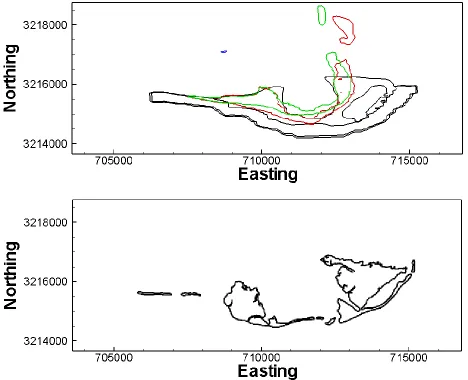
Figure 10: Modified image to compare the barrier outline of the East Island within the barrier system . Top figure represents the initial simulation barrier shoreline footprint.
Bottom figure represents BICM 1998 barrier shoreline footprint post breach. ... 26
Figure 11: Modified image to compare the barrier outline of the Central Island . Top figure represents simulation initial barrier shoreline footprint along with W25 (Red) and
W26 (Green) migration trajectories. Bottom figure represents BICM 1998 barrier
shoreline footprint, with a restoration project of the back barrier marsh of the east
side of the island, landward. ... 27
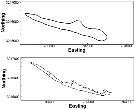
Figure 12: Modified image to compare the barrier outline of the West Island.Top figure represents simulation Initial Barrier Shoreline Footprint. Bottom figure Represents
viii
Figure 13: Polygon parameters in post-simulation completion area and data extraction. The three islands are shown, with an individual polygon per island to ensure proper areas can
be extracted. There are possible limitations due to the closed boundaries of the east
and west, limiting both incoming and exporting sediment transportation throughout
the system. ... 30
Figure 14: Bathymetric Contours at 0m and -0.5m for OCS (W25 Red), NS (W26 Green), Control (W27 Blue). The top represents the 0m contour where the dashed outline is
the original barrier footprint. The bottom represents the -0.5m contour. ... 33
Figure 15: Initial and Final Bed Elevations of W25, W26, and W27. The top figure represents the initial bed elevation prior to simulation start, the following figures are the
resulting bed elevations at simulation completion. ... 34
Figure 16: W25 Bed Load in Water Level Points. 10-Year Increments Show Bed Loss through Time. Beginning at year 0 (initial bed level) in the top left, and sequencing every ten
years accordingly. This shows the varying rates of barrier migration through time. 35
Figure 17: W26 Bed Load in Water Level Points. 10-Year Increments Showing Erosion and Deposition through Time. Beginning at year 0 (initial bed level) in the top left, and
sequencing every ten years accordingly. This shows the varying rates of barrier
migration through time. ... 36
Figure 18: W27 Bed Load in Water Level Points. 10-Year Increments Showing Erosion and Deposition through Time. Beginning at year 0 (initial bed level) in the top left, and
sequencing every ten years accordingly. This shows the varying rates of barrier
ix
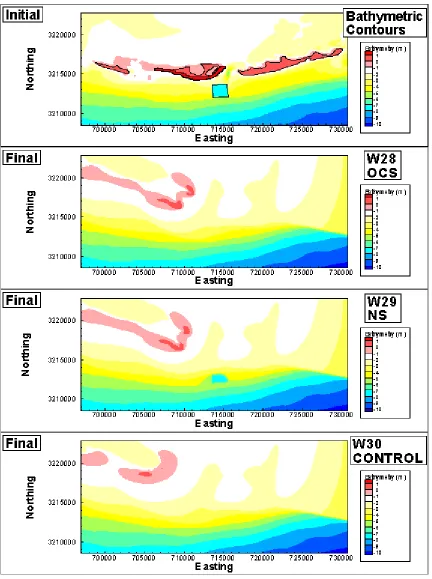
Figure 19: Initial and Final Bathymetries of W28, W29, and W30. The top figure represents the initial bed elevation prior to simulation start, the following figures are the resulting
bed elevations at simulation completion. ... 40
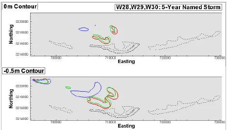
Figure 20: Bathymetric Contours at 0m and -0.5m for OCS (W28 Red), NS (W29 Green), Control (W30 Blue). The top represents the 0m contour where the dashed outline is
the original barrier footprint. The bottom represents the -0.5m contour. ... 41
Figure 21: Initial and Final Bathymetries of W31, W32, and W33. The top figure represents the initial bed elevation prior to simulation start, the following figures are the resulting
bed elevations at simulation completion. ... 44
Figure 22: Bathymetric Contours at 0m and -0.5m for OCS (W31 Red), NS (W32 Green), Control (W33 Blue). The top represents the 0m contour where the dashed outline is
the original barrier footprint. The bottom represents the -0.5m contour. ... 45
Figure 23: Relative Sea Level Rise Comparison between W27 (Control) with RSLR and W34 (Control) without RSLR. This direct comparison shows the effects of RSLR
including the complete subaerial loss of the west island when RSLR is included (top
figure). ... 47
Figure 24: Initial and Final Bathymetries of W35, W36, and W37. The top figure represents the initial bed elevation prior to simulation start, the following figures are the resulting
bed elevations at simulation completion. ... 50
Figure 25: Bathymetric Contours at 0m and -0.5m for NS (W35 Red), OCS (W36 Green), OCS (W37 Blue). The top represents the 0m contour where the dashed outline is the
x
Figure 26: Initial and Final Bathymetries for W41, W42, W43. The top figure represents the initial bed elevation prior to simulation start, the following figures are the resulting
bed elevations at simulation completion. ... 56
Figure 27: Bathymetric Contours at 0m and -0.5m for Control (W41 Red), OCS (W42 Green), NS (W43 Blue). The top represents the 0m contour where the dashed outline is the
original barrier footprint. The bottom represents the -0.5m contour. ... 57
Figure 28: Bathymetric Contours of OCS, NS, and CONTROL, Typical Storm; Named 5-year Storm; Named 20-year Storm Simulation Comparisons. Red- W25, W26, W27;
Green- W28, W29, W30, Blue- W31, W32, W33. This figure indicates a direct
comparison of the remaining footprints when comparing Typical Storm Conditions,
and the Year-5 and Year-20 Named storm events within the OCS, NS, or control
xi
List of Tables
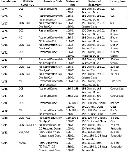
Table 1: Simulation Matrix Parameters and Descriptions.W25-W27 are simulations for Typical Storm Conditions, W28-W30 are simualtions for the named storm at year 5,
W31-W33 are simulations for the named storm at year 20, W34 is the simulation for no
SLR added, and is directly comparable to W27, W35-W37 are simualtions to
compare the effects of grain size variations, W38-W40 are simualtions with an added
3rd sediment class, but the evaluation and results are not discussed in this report,
W41-W43 are simulations that include a renourishment at year 25. ... 18
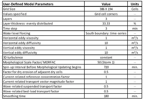
Table 2: User defined model parameters used for all simulations with the exception of W28-W33 which MORFAC was set to 1 only during the named year 5 and year 20 storm
event. ... 21
Table 3: Adaptation of McBride et al., 1992 Louisiana's Barrier Island Shoreline Change Statistic Summary with Simulation Data from W25 (OCS) and W27 (Control).
CWPPRA Barrier Island Areas 1978 and 2002 from Penland et al., 2003. Observed
rates are derived from 1978 and 2002 (24 Year) Area Loss; Model Area Loss is
Derived Directly from Area Extraction. ... 29
Table 4: Percentage Loss of subaerial land for each isobath (m) for each simulation and barrier. The data directly indicates the percentage of each island loss at eavery isobath ... 33
Table 5: Percentage loss at each contour elevation (m) for each simulation and barrier. The data directly indicates the percentage of each island loss at eavery isobath ... 41
xii
Table 7: Percentage loss at each contour elevation (m) for each simulation and barrier. The data directly indicates the percentage of each island loss at eavery isobath ... 47
Table 8: Percentage loss at each contour elevation (m) for each simulation and barrier. The data directly indicates the percentage of each island loss at eavery isobath ... 51
Table 9: Percentage loss at each contour elevation (m) for each simulation and barrier. The data directly indicates the percentage of each island loss at eavery isobath ... 57
xiii
Abstract
Barrier island restoration and nourishment is necessary for sustaining coastal systems
worldwide. In the Mississippi River Delta Plain, the lack of sediment supply, relative sea level
rise, and reworking of abandoned delta lobes promote rapid disintegration of barriers, which can
contribute to mainland storm impacts. Barrier island restorations that utilize higher quality
sediments (Outer Continental Shelf- OCS) are expected to exhibit higher resiliency, withstanding
coastal erosion, event-induced erosion, and ongoing transgression when compared to barriers
nourished using lower quality nearshore (NS) sands. Additionally, use of OCS sediments
increases sediment supply by adding material to the system supporting increased barrier
longevity by maintaining a subaerial footprint longer compared to NS sediments. We used the
Delft3D modeling suite to study barrier geomorphic trajectories nourished using OCS/NS sands,
compared with control simulations with no nourishment. Resulting morphologies from 18
simulations with forcing that included annualized forcing, storms, and SLR are evaluated and
compared.
1
Introduction
Barrier island systems are depositional and erosional coastal landforms that have
significant environmental and ecosystem value (Barbier et al., 2013). Barriers are built vertically,
through wave action and wind processes, and in most settings parallel the coast. Barriers serve
as the primary landform where hurricane waves dissipate their energy and in many instances,
lessen storm surge (Georgiou and Schindler, 2009b; Grzegorzewski et al., 2011). Barrier islands
are found on every continent except Antarctica, in every type of geologic setting, and in every
kind of climate (Davis and FitzGerald, 2008). Barriers occupy 15% of the world’s coastlines
(Cooper and Pilkey, 2004) and are most commonly found on trailing margins. In southeast
Louisiana, barriers are found on either side of the modern Mississippi River Delta (MRD).
Penland et al. (1988) suggested that these landforms are reworked delta deposits, whereby
following nodal avulsion into a new depo-center and in-filling accommodation therein, the
deposits of the previous fluvio-deltaic lobe (channel sands, mouthbars, natural levees) are
gradually reworked by marine processes to form landscapes that resemble arcuate shapes
(headlands) with flanking barrier spits. Storms and other oceanographic processes subsequently
breach, overwash and continue to grow these landscapes (laterally and vertically) until they
detach from mainland (through processes that are presently still unknown), seemingly by
differential and widespread subsidence within the backbarrier setting. Meanwhile, the
accumulation of sands comprising the developing barrier island delay this process and maintain
subaerial exposure through further reworking to form a robust subaerial landform (a barrier
island). The diminishing supply of sand to the system without additional nourishment or
opportunities to recycle local or proximal sand from the system – forces barriers to become
2
The sand volume comprising a barrier (the barrier island lithesome) and the morphology
(planform shape) of a barrier fluctuate over time in response to sediment supply, sea level trends
(Swift 1972, Otvos 1970, 1979,1981,1984; List et al., 1997), the type and size of sediment
comprising the subaerial part of the barrier (Ritchie and Penland, 1988; Rosati and Stone 2009),
the substrate or antecedent geology of the system (Otvos and Carter, 2013; Miner et al., 2007),
and to a large extent the frequency and intensity of storms (Ritchie and Penland, 1988; List et al.,
1997; Miner al., 2009a, Miner et al., 2009b). While barrier islands can occur in both
transgressive and regressive regimes (Short 1999), southern Louisiana barriers are in the
transgressive phase (Miner et al, 2009b, Otvos and Carter, 2013) experiencing some of the
world’s highest rates of barrier island shoreface retreat, disintegration and wetland loss (16.57mi²
per year from 1985 to 2010; Miner et al., 2009b; Couvillion et al., 2011; Georgiou et al., 2005).
To mitigate for barrier island, interior and backbarrier wetland loss, barrier sand
nourishment and marsh creation projects are increasingly becoming necessary for sustaining
coastal systems worldwide. In Louisiana, these projects, along with other structural and
non-structural projects (e.g. levee and ridge construction, sediment diversions; CPRA 2017), form
essential elements of the Louisiana Coastal Masterplan designed to help offset land area loss and
reduce flooding throughout the Mississippi River Delta Plain (MRDP). All of these projects
require substantial economic investment and access to extensive sand resources, a commodity
that is sparse along deltaic coasts. Moreover, the remoteness of barriers requires costly methods
to locate, dredge, transport, and place sand for nourishment, which further complicates the
implementation of cost-benefit analysis and project life-span analysis to ensure a balance of
coastal resiliency and ecological enhancement to maximize the return of investment (McBride
3
Restoration and nourishment projects have basic requirements: adequate sediment
analyses of host barrier, suitable borrow sediment that mimics the host barrier sediment,
adequate volume for replenishment and cut, and assessment of sediment characteristics to enable
barrier longevity (Stauble 2005). Depending on the assessment, often times it may be considered
for the borrow sediment to be slightly coarser than the native sediment to enable greater barrier
longevity (Work et al., 2010). The sediment supply and sediment quality are two of the most
important factors when considering barrier restoration projects for both suitability, retention, and
increased barrier island longevity (Khalil and Finkl 2009). Despite the large economic
expenditure of restoration efforts, they can have a considerable positive impact on (1) the
morphology of the island, (2) the terrestrial and subaqueous habitat proximal and distal to the
barrier, (3) and can have geomorphic benefits throughout the barrier system and the coastline.
Here, we studied the geomorphic benefits of restoration and nourishment efforts utilizing
nearshore sediments (NS) and inner shelf sediments, but consider them asouter continental shelf
(OCS) sediments for this experiment. We examined, over a 50 year window, the effects of grain
size, sand quality, and sea level rise on the final barrier system planform morphology, subaerial
land and intertidal habitat resulting from a restoration effort. We tested the same restoration
footprint under the impact of storms that range from typical frontal weather and extratropical
storms to a large named storm making landfall at year 5 or year 20, and compared all simulations
against control experiments which received no restoration. Experiments using NS sediments
were meant to test nourishment using sediment within the system, while OCS sediment are
testing nourishment with higher sediment quality and size, as well as importing sediment from a
4
products produced through various simulations include barrier shape, erosion and deposition
5
Background and Significance
Regional Study Area
The Isle Dernieres barrier island chain formed from the reworking of an abandoned delta
lobe approximately 400 years BP (Kulp et al., 2005). Within the past 200 years, the barrier chain
transformed from a continuous barrier backed by shallow bays and marshlands to a system with
fragmented barriers separated by multiple inlets, detached from the headland and backed by open
water (McBride et al., 1992; FitzGerald et al. 2018). For the same period the barrier chain
shoreline eroded by more than 2km (McBride et al., 1992; FitzGerald et al. 2018) tidal inlets and
spit platforms grew wider, driven by RSLR and storm-induced wave erosion and storm surge
inundation. Sand once comprising a robust barrier system moved offshore, became sequestered
in ebb-tidal deltas, and moved landward to form flood-tidal deltas. As the Isle Dernieres
migrated onshore, much of the ebb-delta sand moved onshore as well, but some was permanently
lost to the inner shelf (FitzGerald et al., 2018; Miner et al. 2009b). The ongoing process of
barrier landward migration into a deeper backbarrier bay due to SRL continues, and when the
barrier encounters deltaic muds, compaction reduces the barrier footprint (Rosati et al., 2009)
exacerbating barrier retreat due to storm-induced overwash, RSLR, and other attendant
processes. Bathymetric and seafloor-change analysis by Miner et al. (2009a, b) demonstrates that
much of the back-barrier has undergone an increase in water depth from 0 to 1 m during the last
century, attributed to the erosion of bay sediment and RSLR (FitzGerald et al., 2018). McBride
et al (1992), using historical charts and aerial photographs, reported that the width of the island
system decreased by approximately 0.8 km at an average rate of 8.6 m/year (between 1890s and
1988), which contributed toward a total reduction in island area of 27.6 km2, or 78% of the 1890s
6
Islands), this barrier chain is evolving rapidly toward becoming an inner shelf sand shoal (sensu:
Penland et al. 1988), but sand input from updrift sources to the east, coupled with restoration
projects reduces this process to a small degree (FitzGerald et al., 2018). Since 1998, over
50,000,000m³ of sediment have been used for coastal restoration projects on barrier islands in
southern Louisiana utilizing both nearshore and offshore sediment sources (CPRA, 2017).
Nourishment efforts have been key in providing much needed restoration of dune and beach
ridges, backbarrier marshes to sustain the subaerial land of barrier islands and defend against
storms, while the sand influx from the nourishment played a key role to increasing (albeit
short-term) the sediment supply to these barriers and enhancing restorative processes (recurved spit
and spit platform building). For the Isle Dernieres Chain, restoration projects have helped to
mitigate barrier island land loss compared to historic rates, although, ongoing transgression
7
Objectives
The primary objectives for this research entail understanding and quantifying the
long-term geomorphic benefits (and thus economic benefits) of nourishment and restoration projects
that utilize OCS sediments and compare to projects that utilize NS sediments. The study
considered benefits that are purely derived based on the different properties between the two
sediment types corresponding to using OCS or NS (e.g., grain size and fines content). A second
objective of this study was to assess the geomorphic benefits between OCS and NS sediment
with respect to the regional sediment budget, and specifically that OCS sources add sediment to
the coastal system, while NS sources typically mine sediment from within the system.
To achieve research objectives we utilized the hydrodynamic, sediment transport and
morphology modeling suite, Delft3D (Deltares, 2015), developed a model domain that included
a barrier island chain (three islands). A developed simulation matrix includes: (1) a restoration
template using OCS and NS sediments as well as control, (2) use of various grain size
differences between OCS and NS sediments, (3) an assessment of the role of tides, waves, storms
and the effects of sea level rise (SLR) on the resulting barrier morphology, (4) and the effect of a
8
Hypotheses
Barrier island restoration and nourishment are necessary actions for sustaining coastal
systems in areas where anthropogenic modifications to the coastal system or watershed have
reduced the ability for barriers to recover naturally from disruptions such as storms and
accelerated sea level rise. In the Mississippi River Delta Plain (MRDP), the lack of sediment
supply and ongoing transgression promotes rapid disintegration of barriers, which can contribute
to mainland storm impacts and compromise the stability of estuaries.
The following hypotheses are tested as part of this research:
Hypothesis 1: Barrier island restorations that utilize higher quality sediment (Outer Continental Shelf – OCS) are expected to exhibit higher resiliency withstanding erosion during
storms and the ongoing transgression, compared to lower quality near shore (NS) sands.
Description: OCS sands are higher quality. The grain size, high sand content and low
mud/silt content enables barriers to better maintain their subaerial and intertidal footprint through
time, when subjected to coastal forcing. Barriers without nourishment are more prone to
overwash, rapid transgression, and significant sediment deficits, while barriers that use NS
sediment for nourishment will exhibit less resilience compared to those that use OCS sediments.
Hypothesis 2: Barrier island nourishment and restoration projects that utilize OCS sediments help offset low sediment supply (locally and regionally) by adding material to the
littoral system, and help increase barrier longevity compared to their NS counterparts that use
sand from within the active littoral system, contributing overall to both the subaerial and
9
Description: The geomorphic contribution of sediment from outside the system supplies
sediment, enhances sediment transport, promotes sediment mobility and naturally nourishes the
subaerial portion of the barrier and nearshore habitat through active littoral zones. Without
additional sediment input, barrier transgression will continue threatening the overall barrier
10
Materials and Methods
Numerical Modeling
Barrier island modeling was conducted using Delft3D, a multi-dimensional,
physics-based morphodynamic model that simulates both two and three dimensional flow, wave,
sediment transport, and bed morphology/bathymetry. These factors are included for both
hydrodynamics and aeolian transport. Delft3D has been widely used to simulate hydrodynamic
and morphodynamic processes along with hurricane-induced sediment transportation (Hu et al.,
2015). This numeric model solves depth-integrated equations of motion using conversion of
mass and momentum principles (Lesser et al., 1994, Deltares, 2015). Through this research,
Delft3D-FLOW and Delft3D-WAVE modules perform in a coupled approach for hydrodynamic
computations while simultaneously updating the bathymetry.
Delft3d-FLOW simulates tidal and wind influences on water currents while continuously
updating the water level, changes in velocity, and bed elevation. Delft3D-WAVE simulates wave
computation through SWAN (Simulating Waves Nearshore). The model first computes the wave
direction followed by shoreward propagating waves. SWAN is couple with depth-averaged
non-linear flow to describe wave propagation, breaking, and diffraction (Deltares 2013; Reniers et al.,
2004). Bedload elevation (alterations in the bathymetry) are updated following the hydrodynamic
results computing suspended and bedload transport (Caldwell and Edmonds, 2014).
Sediment transportation, erosion, and deposition are calculated in accordance with, but
separately from FLOW and WAVE. Delft is able to compute both cohesive and noncohesive
sediments, but in this research, the marginal fraction of noncohesive sediments used exclude
11
Suspended sediment transport is computed through the three-dimensional depth-averaged
advection-diffusion equation:
where ci is mass concentration of the sediment fraction (kg/m³), while assuming a
standard Rouse profile concentration gradient, ux, uy, and uz are the x-, y-, and z-directed fluid
velocities (m/s). Ws,i is assumed as the settling velocity of the sediment fraction (m/s), and εs,x,i,
εs,y,i, and εs,z,i are directional eddy diffusivities of the sediment fraction (m²/s).
Settling velocities of noncohesive sediments are calculated to Van Rijn (1993) dependent
upon grain diameter in suspension:
Where R is the submerged specific gravity (ps/pw-1), ps is the specific density of sediment
(kg/m³), pw is the specific density of water (kg/m³), g is the acceleration due to gravity (9.81m/s²)
Di is the grain size diameter of the sediment fraction (m), and v is the kinematic viscosity
coefficient of water (m²/s). Noncohesive suspended sediment exchange with the bedload is
computed as an erosive flux due to upward diffusion and depositional flux due to sediment
12
Where α2(ℓ) is the sediment concentration correction factor, εs(ℓ) is the sediment diffusion
coefficient evaluated at the cell of the sediment fraction. ca(ℓ) as the reference concentration of
the sediment fraction, ckmx(ℓ) as the average concentration of the cell of sediment fraction, and ∆z
is the difference between the center of the cell and the Van Rijn reference height: ∆z=zkmx- α.
The approximated depositional flux with D(ℓ) as the representative diameter of the
suspended sediment, which is more commonly referred to as the D50. Depositional flux due to
sediment settling is given by:
The first term of this equation is implemented as the sediment source term; the second is
implemented as the (positive) sink term.
The total depositional source and sink terms are then justified and guaranteed to project
13
The bedload, or total load transport is computed for all sediment fractions through
calculating the magnitude and direction of the bedload transport at the cell centers using the
transportation formula. The transport rates at the cell interfaces iare then determinedand
corrected according to bed-slope, upwind in bed composition, and available sediment (Deltares,
2014).
Bedload transport is then calculated through Van Rijn (1993):
Where qb,i is bedload sediment discharge per unit of the sediment fraction (m²/s), u is the
depth-averaged velocity (m/s), and uc,i is the critical depth averaged velocity (m/s) for initiation
of motion of the sediment fraction. The direction of the bedload transport is determined by the
local flow conditions and then adjusted for bed-slope effects (Bagnold, 1966; Ikeda, 1982). The
suspended load transport entering the upstream open boundary is labeled as a boundary
14
Model Domain, Model Set-up, and Initial Conditions
A curvilinear grid (Figure 2) was developed with the Deltares GUI through RFGrid and Quicken. The grid covering the bathymetry is 386 cells (x-axis) by 194 cells (y-axis) equating to
approximately 54,596 m wide and 21,320 m high. The grid has variable cell sizes with higher
cell refinement in the areas of interest near the barriers (Figure 3) along the central, longitudinal
margin (~20m), while offshore the cells size is approximately 1-2 km.
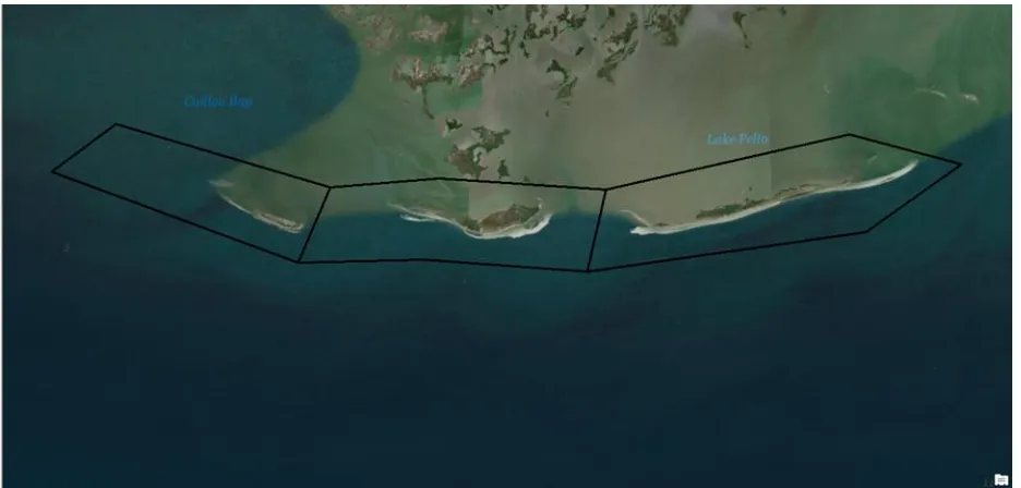
To avoid using a schematized basin, the domain and bathymetry used in the model were
informed from the Isle Dernieres barrier island chain in southwest Louisiana (Figure 1). We used
the 1980s bathymetry collected by the National Oceanic and Atmospheric Administration
(NOAA) as processed for the Barrier Island Comprehensive Monitoring Program (BICM) by
Miner et al., (2009), and List et al., (1997) as this was a period when the barriers were more
robust and had not received any type of nourishment at the time. In addition, selecting this period
allows for some form of morphodynamic validation, as more recent results in the 1990s and early
2000s are available for comparison.
15
We utilized the same domain and initial bathymetry for all model simulations with three
variances. For each variance, the bathymetry was updated to reflect a nourishment using OCS,
NS, and a control where no changes in the bathymetry were implemented (Figure 4). For
simulations were nourishment used OCS sediments, the dune and beach of the central barrier
was restored using approximately 10.7 million m³ of sand with median grain diameter of
160.01µm. The background median grain diameter of the barrier lithosome was defined at
156µm for all simulations per field results (Georgiou, 2017, and Kindinger et al., 2014). For
simulations were NS sediments were used the central barrier was once again nourished using the
same restoration template as the OCS, but the sediment used to fill the template had a median
grain diameter that was the similar to the background (~150µm) and the material used originated
from a dredged pit located on the distal ebb tidal delta. The control experiment utilized the initial
bathymetry without any modification (e.g., no restoration and no dredge pit). In order to track
sediment dispersal patterns, we used two sediment classes that were either different (e.g., 156µm
and 160µm), or if similar, the restoration template was filled with sediment that was fractionally
16
Figure 2: Curvilinear grid developed from the Deltares RFGrid and Quicken. The grid is 386 cells (x-axis) by 194 cells (y-axis) which equates to approximately 54,596 m wide and 21,320 m deep. There are variable cell sizes in the central section.
17
Figure 4: OCS, NS, and Control Initial Bathymetry with the Subaerial (0m) Footprint Outlined. The OCS has only the central barrier nourishment added. The NS has the central barrier
18
Table 1: Simulation Matrix Parameters and Descriptions.W25-W27 are simulations for Typical Storm Conditions, W28-W30 are simualtions for the named storm at year 5, W31-W33 are simulations for the named storm at year 20, W34 is the simulation for no SLR added, and is directly comparable to W27, W35-W37 are simualtions to compare the effects of grain size variations, W38-W40 are simualtions with an added 3rd sediment class, but the evaluation and
19
Boundary Conditions
To build the most representative model simulations, we drove the model at the offshore
boundary with hourly tidal, subtidal, wind, and wave data. Wind and wave data were obtained
from the Wave Information Study (WIS) which is an online database containing hourly wind and
wave data beginning in January, 1980. Each simulation uses WIS data from the year 2000, in
which there were no major storm events. This was intentional to avoid unrealistic
morphodynamic response resulting from a large storm because of the use of morphodynamic
upscaling (MORFAC). Tidal data for the same year (2000) were from the NOAA Grand Isle
station (Station 73125). Each set of simulations were assessed for OCS, NS, and Control with
these boundary conditions, and were repeated with the presence of a named storm simulating a
tropical cyclone at a selected year. For instance, for simulations W28-W33, a hurricane was
forced upon the system to simulate the geomorphic effects resulting for such an event and the
possible impacts on the barrier land area trajectory. We selected Hurricane Lili as a
representative event, which made landfall in southern Louisiana on October 3rd, 2002 as a
category 3 with peak winds reaching 145mph.. During the modeling experiment, the simulated
effect was intended to represent a hurricane making landfall at year 5 (hereafter Year 5 storm),
and year 20 (hereafter Year 20 storm). We stopped the original simulation at year 5 and year 20
respectively, and then simulated Hurricane Lili with full sediment transport and morphology and
a MORFAC of 1, after which we continued the simulation to the end. Finally, additional
simulations were carried out to study the effect of larger grain size differences between
background sediment and OCS or NS, as well as had varying parameters including greater grain
size deviations, additional sediment classes, and a renourishment at year 25. The defined set
20
altered parameters than the set Delft3D parameters. A morphological acceleration or upscaling
factor (MORFAC) is imposed upon each of the simulations. The morphological upscaling factor
is a method used to increase the timescales of sediment transportation through an increase in bed
level alterations from each hydrodynamic time step by the acceleration factor (Lesser et al.,
2004). The morphodynamic upscaling significantly decreases the computational time per
simulation and simulates an extension in total length of the time simulated. This research entails
a MORFAC of 50, which projects 50 years on every run excluding the storm event in W28-W33,
which ran with a MORFAC of 1. Every simulation began from a period of rest, with a
morphological spin-up interval of 720min. Bed layers and sediment thickness were evenly
21
Table 2: User defined model parameters used for all simulations with the exception of W28-W33 which MORFAC was set to 1 only during the named year 5 and year 20 storm event.
Time series water level data were derived from NOAA Grand Isle tidal gauge station for
the year 2000. Additionally, relative sea level rise (RSLR) was added to every simulation except
for W34, which is used as a direct control comparison to W27. The 50-year outlook necessitates
accurate depiction of sea level trends. We applied RSLR as a linear increase of 40 cm over the
50 year water level projection which was derived from the CPRA (2017) 1-m scenario of
predicted relative sea level rise 1992-2100. Wave and wind data were gathered through the Army
Corp of Engineers, Wave Information Studies (WIS) database. BICM (1998) shoreline
bathymetry was used for result comparisons. Open boundaries extend the entire length of the
22
transport and waves) but Newman for tides. The Northern boundary is closed to any forcing
parameters (Figure 5). Offshore directed waves with a northerly component were ignored, but
winds from all azimuth were considered (Figure 6, Figure 7, Figure 8, Figure 9).
Figure 5: Model Boundary Conditions- Open (red) and Closed (black) Boundaries for Offshore and Lateral Tides, Waves, and Subtidal Water Level Variations [f(x,t)]. The open boundary allows for all water, wind, and tide level fluctuations through the system. The limitations of computational power negate the use of open boundaries along the east and west, and have negative implications for the flux of sediment migration along with not allowing additional sediment input through the system, as would be typical in a normal barrier system.
Modeling of the various scenarios (non-storm activity, storm at 5 years, and storm at 20
year variances) was intended to represent and investigate relative conditions. Hurricane
development varies every year, with major events randomly occuring through a given 50-year
period, thus the 5-year and 20-year hurricane representation. The variances also allow
investigation of alterations to the general bathymetry, NS and OCS sediment comparison, and
23
Figure 6: Wave Record over 50-year Simulation Period. Years 0-50 are along the x-axis and wave height (m) along the y-axis. The wave data is collected from a one-year timespan. With the MORFAC set to 50, the data is repeated 50 times.
Figure 7: Wind Record over 50-year Simulation Period. Years 0-50 are along the x-axis and wind speed (m/s) along the y-axis. The wind data is collected from a one-year timespan. With the MORFAC set to 50, the data is repeated 50 times.
24
Figure 9: Named 5-Year and 20-Year Storm Event Water Level Record. Time span of 5.12 Days, with maximum water level at 1.02m.
Model Validation
The model was validated with observations to ensure that shoreline erosion, subaerial
land, and where available, overall morphology of the barrier islands simulated by the model
reproduced observations. The named storm applied during the experiments at year 5 and year 20
respectively was Hurricane Lili, which impacted the Isle Derniere Islands. Subaerial land from
the simulations was compared with observations (Penland et al., 2003). The model simulated
erosion that resulted in approximately 17% loss of subaerial land as a result of the storm, which
compares favorably to observations of 19-20% loss (Penland et al., 2003). For the longer-term
morphology of the islands, the model was again compared to observation using data reported by
McBride et al. (1992) and Penland et al. (2003). Because exact bathymetry over 50 years was not
available to test the model performance from 1980-2030, we selected to test model skill using
shoreline erosion rates, loss of subaerial land (total loss and average rate of loss), and visually
compare island shape at selected times where imagery was available; this process is challenging
as the Isle Dernieres received restoration numerous times, as opposed to our experiments where
restoration only takes place once.
The long term projected disappearance from McBride et al., 1992 (Table 3) directly
25
central island average loss rate of 16.5 ac/yr which corresponds with loss rates reported by
McBride (1992) between 9.1 and 31.4 ac/yr for a 15 and 100 year period respectively. Various
factors differed among simulations and created a range of outputs that resulted in variable loss
rates among simulations. The first nine simulations within the matrix were considered
comparable and indicated results that are most similar to observations. There were used for
model validation. Furthermore, Penland et al. (2003) through an assessment of CWPPRA
restoration projects provided additional information that can be used for model validation which
includes area loss over time, post-restoration disappearance date (or years from restoration), and
the projected added barrier survivability in the out years. Their study reports survivability that is
of the same order as that predicted by our model simulations and approximately 8-15 years with
26
27
28
Figure 12: Modified image to compare the barrier outline of the West Island.Top figure
29
Table 3: Adaptation of McBride et al., 1992 Louisiana's Barrier Island Shoreline Change
Statistic Summary with Simulation Data from W25 (OCS) and W27 (Control). CWPPRA Barrier Island Areas 1978 and 2002 from Penland et al., 2003. Observed rates are derived from 1978 and 2002 (24 Year) Area Loss; Model Area Loss is Derived Directly from Area Extraction.
Barrier Response Evaluation Metrics
Following each simulation, results were processed for both numeric and visual
representation using various metrics.
Area calculation was accomplished with a Matlab© script which reads the simulation
results file (.trim file) and the pre-determined polygons (Figure 13) that define the system
boundary. Each polygon represents the respective west, central, or eastern barrier. Area is
extracted to a spreadsheet where area in m² is converted to acres, and isobath elevations ranging
from subaqueous to subaerial (-2m, -1.5m, -1.0m, -0.5m, 0m, and 0.5m) are evaluated. From
these data, individual barrier erosion or deposition rates are calculated along with % loss and
acre per year loss. A subsample function (MOd; remainder after division of dividend by the
divisor) is utilized to gain an accurate sample representation of yearly data (one data sample per
30
Tecplot© is used for visualizing bed level in water level points (bathymetry) and
cumulative erosion and deposition. Although further explored in the Results and Discussion,
these visual figures confirm a variety of barrier system components including erosion,
deposition, within-system sediment transportation, barrier migration, spit platform development
and evolution, inlet habits, and flood and ebb delta deposits.
31
Results
The results from the simulation matrix are reported in this section for each set of
experiments testing specific set of conditions reported previously in Table 1. The first section
outlines results from the typical storm conditions experiments, followed by results from the
simulations that considered a named storm making landfall in year 5 and 20 respectively, and
finally results that depict the effect of grain size - between the OCS sand source and the local
sand - on barrier morphology, as well as the role of relative sea level rise and re-nourishment on
barrier morphology.
Typical Storm Conditions
Typical storm conditions are the relative simulations which can then be compared to
similar simulations in the following results. Barriers nourished with OCS sand (W25) (Figure 16)
maintained the largest and more robust subaerial footprint compared to experiments nourished
with NS (W26) sands and the control (W27) (Figure 17 and Figure 18). The OCS subaerial
barrier footprint for the central barrier (where sand was placed) experienced an average loss of
~25 acres per year (ac/yr.) with peak loss rates occurring from year 0 to year 20, and then from
year 40 to year 50 (for OCS). The barrier nourished with NS sand experienced a loss of
~26ac/yr, with peaks loss rates for the same periods as OCS. During the control experiment, the
central barrier eroded at an average rate of ~17ac/yr; while this loss rate is less than OCS and
NS, the subaqueous elevations experience a higher loss rate of up to 37ac/yr (Figure 15). The
east (updrift) island experienced a complete loss of subaerial land by the end of the simulation
period, while the central and west islands suffered a 69% and a near total loss (~99%)
respectively The NS east and west (downdrift) islands experienced a complete loss of subaerial
32
migrated landward towards the northwest for both OCS and NS, approximately 500m and 750m
respectively, while the barrier in the control experiment migrated approximately 1,500m and lost
subaerial exposure at year 43. We observed barrier shoreline erosion and upper shoreface
deposition in all three experiments for years 0 through 20, at magnitudes corresponding to trends
similar to barrier migration. Barrier landward migration for all simulations slowed between years
10 to 30 which resulted in enhanced recurved spit formation. By year 40, the spit platform that
initially joined the central and west islands was breached and detached forming a wide inlet
between the islands. The central barrier was subjected to major overwash at year 40 through 50.
Landward migration and rollover for OCS and NS experiments was highest between year 40 and
50, while for the control experiment landward migration and rollover was initiated earlier in the
simulation between year 30 to 50 and, at a rate of 2 and 3 times the OCS and NS rates,
respectively. By the end of the simulation (year 50) half of the dredge pit in NS experiment was
filled, and for all experiments the inlet separating the central and east island infilled, whereas the
33
Figure 14: Bathymetric Contours at 0m and -0.5m for OCS (W25 Red), NS (W26 Green), Control (W27 Blue). The top represents the 0m contour where the dashed outline is the original barrier footprint. The bottom represents the -0.5m contour.
Table 4: Percentage Loss of subaerial land for each isobath (m) for each simulation and barrier. The data directly indicates the percentage of each island loss at eavery isobath
% Loss
Elev (m) -2.00 -1.50 -1.00 -0.50 0.00 0.50W25 East 42.13 71.59 99.55 100.00 100.00 100.00
OCS Central 9.11 23.68 47.37 54.60 68.75 80.66
West -17.45 -10.65 18.96 37.28 98.95 100.00
W26 East 42.46 71.78 99.83 100.00 100.00 100.00
NS Central 11.33 25.06 48.62 57.32 71.52 84.49
West -17.70 -10.77 20.15 37.22 100.00 100.00
W27 East 43.11 71.89 100.00 100.00 100.00 100.00
CONTROL Central 23.88 32.30 63.26 73.57 99.09 100.00
34
Figure 15: Initial and Final Bed Elevations of W25, W26, and W27. The top figure represents the initial bed elevation prior to simulation start, the following figures are the resulting bed elevations at simulation completion.
35
36
Figure 17: W26 Bed Load in Water Level Points. 10-Year Increments Showing Erosion and Deposition through Time. Beginning at year 0 (initial bed level) in the top left, and sequencing every ten years accordingly. This shows the varying rates of barrier migration through time.
37
38
Year-5 Named Storm Event
Barriers nourished with OCS (W28) sand maintained the largest and more robust
subaerial footprint compared to experiments nourished with NS (W29) sands and the control
(W30) (Figure 19). The OCS subaerial barrier footprint for the central barrier experienced an
average loss of approximately 30ac/yr with peak loss rates occurring from year 0 to year 20. The
barrier nourished with NS sands experienced a loss of approximately 110ac/yr with a peak loss
rate immediately following the induced storm at year 5. During the control experiment, the
central barrier eroded at an average rate of 10ac/yr, with subaqueous elevations experiencing
higher loss rates up to 390ac/yr. The OCS and NS east (updrift) and west (downdrift) islands
experienced a complete loss of subaerial land by the end of the simulation period, while the
central island suffered a 71% (OCS) and 75% (NS) loss (Table 5). The west and central barriers
migrated landward towards the northwest for both OCS and NS, approximately 1,500m and
1,600m respectively, while the barrier in the control experiment migrated approximately 3,800m
and lost subaerial exposure at year 45. We observed barrier shoreline erosion and upper
shoreface deposition in the OCS and NS experiments for years 0 through 20 at magnitudes
corresponding to trends in barrier migration. The control experiment resulted with shoreface
deposition in the first 5 years, followed by shoreline erosion through the subsequent 45 years.
Migration for OCS and NS simulations slowed between years 20 to 30, resulting in recurved spit
formation. By year 30, the spit platform merging the central and west islands migrated with the
barriers at a similar rate. The central barrier was subjected to major overwash events from year
10-20 and from year 40 through 50. Landward migration and rollover for OCS and NS
experiments was highest between year 30 and 50, while for the control experiment land
39
OCs and NS. By the end of the simulation (year 50) more than half of the dredge pit in the NS
experiment were filled, and for all experiments, the inlet separating the central and east island
infilled. The spit platform between the central and west barrier resisted erosion and was present
through the end of the simulation period for both OCS and NS experiments, while for the control
experiment, the spit platform was breached and detached around year 40, forming a wide shallow
40
Figure 19: Initial and Final Bathymetries of W28, W29, and W30. The top figure represents the initial bed elevation prior to simulation start, the following figures are the resulting bed
41
Figure 20: Bathymetric Contours at 0m and -0.5m for OCS (W28 Red), NS (W29 Green), Control (W30 Blue). The top represents the 0m contour where the dashed outline is the original barrier footprint. The bottom represents the -0.5m contour.
Table 5: Percentage loss at each contour elevation (m) for each simulation and barrier. The data directly indicates the percentage of each island loss at eavery isobath
% Loss
Elev (m) -2.00 -1.50 -1.00 -0.50 0.00 0.50W28 East 30.32 97.66 100.00 100.00 100.00 100.00
OCS Central 32.96 43.50 61.41 62.56 71.14 96.86
West 39.14 88.59 100.00 100.00 100.00 100.00
W29 East 30.96 98.26 100.00 100.00 100.00 100.00
NS Central 35.84 47.88 64.62 68.05 75.24 97.70
West 36.59 87.02 100.00 100.00 100.00 100.00
W30 East 31.99 98.52 100.00 100.00 100.00 100.00
CONTROL Central 45.90 69.89 100.00 100.00 100.00 100.00
42
Year-20 Named Storm Event
Barriers nourished with OCS sand (W31) maintained the largest and more robust subaerial footprint compared to experiments nourished with NS sands (W32) and the control (W33) (Figure 21). The OCS subaerial barrier footprint for the central barrier experienced an average loss of approximately 58ac/yr with peak loss rates occurring from year 20 to year 30. The NS sands experienced a loss of approximately 77ac/yr with a peak loss rate occurring from year 20 to 30. During the control experiment, the central barrier eroded at an average rate of 10ac/yr, with subaqueous elevations experiencing higher loss rates up to 413ac/yr. The OCS and NS east (updrift) and west (downdrift) islands experienced a complete loss of subaerial land by the end of the simulation period, while the central island suffered a 77% (OCS) and 82% (NS) loss (Table 6
Table 6: Percentage loss at each contour elevation (m) for each simulation and barrier. The data directly indicates the percentage of each island loss at eavery isobath
). The west and central barriers migrated landward towards the northwest for both OCS
and NS, approximately 1,400m and 1,500m respectively, while the barrier in the control
experiment migrated approximately 4,000m and lost subaerial exposure at year 35, with
reemergence at year 39 to 43, and complete loss through the remaining years. We observed
barrier shoreline erosion and upper shoreface deposition in the OCS and NS experiments for
years 0 through 20. The control experiment resulted with shoreline erosion and shoreface
deposition through the first 20 years, followed by intense shoreline erosion through the
subsequent 30 years. Migration for OCS and NS simulations slowed between years 30 and 40,
resulting in recurved spit formation. By year 40, the spit platform merging the central and west
islands migrated with the barriers at a similar rate. The central barrier was subjected to major
overwash from year 20 through 40. Land migration and rollover for all three experiments was
highest between year 30 and 50. The control experiment had migration and rollover rates over
2.5 times the OCS and NS. By the end of the simulation (year 50) the majority of the pit in the
NS experiment was filled, and for all experiments, the inlet separating the central and east island
43
OCS and NS experiments, but was breached in the control experiment, and detached around year
44
Figure 21: Initial and Final Bathymetries of W31, W32, and W33. The top figure represents the initial bed elevation prior to simulation start, the following figures are the resulting bed
45
Figure 22: Bathymetric Contours at 0m and -0.5m for OCS (W31 Red), NS (W32 Green), Control (W33 Blue). The top represents the 0m contour where the dashed outline is the original barrier footprint. The bottom represents the -0.5m contour.
Table 6: Percentage loss at each contour elevation (m) for each simulation and barrier. The data directly indicates the percentage of each island loss at eavery isobath
% Loss
Elev (m) -2.00 -1.50 -1.00 -0.50 0.00 0.50W31 East 31.42 96.67 100.00 100.00 100.00 100.00
OCS Central 30.80 40.00 55.89 58.53 77.15 95.03
West 31.49 77.86 100.00 100.00 100.00 100.00
W32 East 31.85 97.27 100.00 100.00 100.00 100.00
NS Central 35.00 45.14 61.44 65.15 81.45 96.95
West 28.40 75.87 100.00 100.00 100.00 100.00
W33 East 32.39 97.85 100.00 100.00 100.00 100.00
CONTROL Central 45.78 69.51 100.00 100.00 100.00 100.00
46
Role of RSLR
We performed experiments with and without RSLR for the control setup only. A total of
40cm of sea level rise (SRL) (CPRA, 2017) was applied over the 50 year period, applied linearly
over the simulation period. Simulations with Relative Sea Level Rise (RSLR) experienced higher
subaerial loss compared to simulations without the addition of RSLR (W34) (Figure 23). The
subaerial footprint for the central barrier for the simulation with SLR experienced an average
loss of approximately 17ac/yr while the simulations without SLR experienced an average loss of
approximately 15ac/yr. Barrier islands for the simulation with SLR experienced a complete loss
of subaerial land (east and west islands), and a near complete loss of the central island (99%) by
the end of the simulation period. All barrier islands for the simulation without SLR maintained
subaerial land through year 50, with loss of subaerial land at approximately 28% for the west
island, 82% for the central island, and 98% loss for the east island (Table 7). Both experiments
resulting in total barrier island landward migration towards the northwest at approximately
1,500m (with SLR) and 1,100m (without SLR). Both simulations showed barrier shoreline
erosion and upper shoreface deposition for years 0 through 20. Between years 10 to 30, barrier
island migration slowed, at which point recurved spit formation increased, and spit platform
development accelerated. Simulations without SLR resulted in more recurved spit development,
spit elongation and continued spit platform development, whereas simulations with SLR resulted
in breaching of spit platforms and less spit formation and extension. Experiments with SLR also
experienced more overwash and thus more landward barrier migration and rollover (year 30-50)
at rates of nearly 1.4 times more compared to experiments without SLR. In both experiments, the
47
Figure 23: Relative Sea Level Rise Comparison between W27 (Control) with RSLR and W34 (Control) without RSLR. This direct comparison shows the effects of RSLR including the complete subaerial loss of the west island when RSLR is included (top figure).
Table 7: Percentage loss at each contour elevation (m) for each simulation and barrier. The data directly indicates the percentage of each island loss at eavery isobath
% Loss
Elev (m) -2.00 -1.50 -1.00 -0.50 0.00 0.50W27 East 43.11 71.89 100.00 100.00 100.00 100.00
CONTROL Central 23.88 32.30 63.26 73.57 99.09 100.00
West -17.25 -11.88 14.16 35.98 100.00 100.00
W34 East 45.26 79.41 89.39 94.19 98.39 100.00
CONTROL Central 24.81 42.17 50.57 45.10 81.72 100.00
48
Effects of Grain Size Variation
Barriers nourished with OCS sand with the restoration footprint median grain size of
165µm (W36) maintained the largest and more robust subaerial footprint compared to
experiments nourished with OCS sands at 200µm (W37) and NS sands at 150µm (W35) (Figure
24). The NS subaerial footprint for the central barrier experienced an average loss of
approximately 19ac/yr. The subaerial footprint for OCS experiment (200µm) experienced an
average loss rate of 25ac/yr, and OCS experiment (165µm) experienced 18ac/yr loss. Peak loss
rates for all three experiments occurred from year 0 to 20, and then from year 40 to 50. For each
experiments east (updrift) and west (downdrift) island experienced a complete loss of subaerial
land by the end of the simulation period, with the exception of OCS experiment (165µm) with a
near complete loss (99%), and OCS (200µm) with complete subaerial loss of all three islands.
The NS experiment central island had a loss of 75%, OCS (165) loss of 65% (Table 8). The west
and central barriers migrated landward towards the northwest for all three experiments, with
OCS (165µm) at approximately 100m, OCS (200µm) at 250m, and NS at 500m. We observed
barrier shoreline erosion and upper shoreface deposition in all three experiments for years 0
through 20, at magnitudes corresponding to trends in barrier migration. Migration trends for all
barriers were similar to other simulations with the exception of the NS experiments, where the
central island had an additional spit breach towards the north. The OCS (165µm) experiment
maintained the elongated spit, while the OCS (200µm) experiment did not maintain the subaerial
spit platform. The central barrier was subjected to major overwash at year 40 through 50, but all
three experiments maintained a fragmented, minimal trace of the restoration footprint. Landward
migration and rollover was highest between year 40 and 50 for all experiments, but with the NS
49
dredge pit in the NS experiment was filled, and for all experiments the inlet separating the
central and east island infilled. The inlet separating all the central and west islands widened post
50
Figure 24: Initial and Final Bathymetries of W35, W36, and W37. The top figure represents the initial bed elevation prior to simulation start, the following figures are the resulting bed
51
Figure 25: Bathymetric Contours at 0m and -0.5m for NS (W35 Red), OCS (W36 Green), OCS (W37 Blue). The top represents the 0m contour where the dashed outline is the original barrier footprint. The bottom represents the -0.5m contour.
Table 8: Percentage loss at each contour elevation (m) for each simulation and barrier. The data directly indicates the percentage of each island loss at eavery isobath
% Loss
Elev (m) -2.00 -1.50 -1.00 -0.50 0.00 0.50W35 East 41.63 71.56 100.00 100.00 100.00 100.00
NS Central 11.67 26.27 48.51 59.58 75.45 85.70
West -17.44 -10.91 20.34 36.69 100.00 100.00
W36 East 41.76 71.26 100.00 100.00 100.00 100.00
OCS Central 8.91 24.39 46.11 53.69 65.06 79.00
West -17.68 -10.41 19.61 36.66 98.95 100.00
W37 East 38.77 71.33 99.86 100.00 100.00 100.00
OCS Central 10.44 22.39 36.69 35.25 47.56 64.36
52
Year 25 Re-nourishment
Barriers nourished with OCS sands (W42) maintained the largest and more robust
subaerial footprint compared to experiments nourished with NS sands (W43) and the control
(W41) (Figure 26). The OCS subaerial footprint for the central barrier experienced an average
loss of 8ac/yr compared to 9ac/yr for the NS sand experiment. The OCS east island experienced
a complete loss of subaerial land by the end of the simulation period, while the central and west
islands suffered a 23% and 76% loss, respectively. The NS east and west islands experienced a
complete loss of subaerial land while the central island suffered a 26% loss (Table 9). The west
and central barriers migrated landward towards the northwest for all experiments; the OCS
migrated 1,400m and the NS at 1,500m. Shoreline erosion and upper shoreface depositions
trends were similar to other simulations, with additional overwash (between year 40 and 50) and
53
Implications for Barrier Island Restoration
Barrier island restoration using OCS sediment contributes to add sediment supply to the
system. This contribution offsets the present system sediment deficit, helps prolong the barrier
footprint, and reduces transgressive submergence. Variations in the success of nourishment
efforts depend primarily on two factors: higher sand quality and coarser sediment size, both of
which contribute to extend the restoration project lifespan and enhance regional sediment
transport. There is a non-linear response between grain diameter and barrier island area when
compared to a reference scenario when NS sediments were used (156 µm). For instance a 6.5%
increase in D50 (160µm) corresponds to a 40% retention in the barrier island area. Similarly, a
9.5% and a 32% increase in the D50 (165 and 200µm) corresponds to a retention in the barrier
island areas of the order of ~50% and ~130% respectively. Barrier restoration/nourishment with
NS sediments exhibit higher landward migration and appear more susceptible to storm-included
transport, mobilizing sediment across the barrier platform, creating elongated spits, and
experiencing more frequent overwash and re-working. These processes gradually change when
coarser sediment is used for nourishment. These barriers display lower landward migration, are
less susceptible to storm-induced sediment transport, and exhibit less overwash and split
breaching. This is likely due a robust dune ridge that hinders wave run-up and inundation during
high water level events, which helps redirect storm surge around the barrier reducing rollover
(Georgiou and Schindler, 2009a). Barrier splits and spit platforms are more resistant to
breaching, likely because they have sufficient berm elevation and subaerial exposure to prevent
incision. The contribution of sediment from an outside source increases sediment supply to the
system. The benefits of adding sediment to the system was obvious during our simulations.

![Figure 5: Model Boundary Conditions- Open (red) and Closed (black) Boundaries for Offshore and Lateral Tides, Waves, and Subtidal Water Level Variations [f(x,t)]](https://thumb-us.123doks.com/thumbv2/123dok_us/8921315.1841749/36.612.73.520.199.408/figure-boundary-conditions-boundaries-offshore-lateral-subtidal-variations.webp)