DESIGNING RELIABLE HIGH-PERFORMANCE STORAGE SYSTEMS FOR HPC ENVIRONMENTS

(1)

STORAGE SYSTEMS FOR HPC ENVIRONMENTS

by

Lucas Scott Hindman

A thesis

submitted in partial fulfillment of the requirements for the degree of Master of Science in Computer Science

Boise State University

(2)

(3)

DEFENSE COMMITTEE AND FINAL READING APPROVALS

of the thesis submitted by

Lucas Scott Hindman

Thesis Title: Designing Reliable High-Performance Storage Systems for HPC Envi-ronments

Date of Final Oral Examination: 06 August 2011

The following individuals read and discussed the thesis submitted by student Lucas Scott Hindman, and they evaluated his presentation and response to questions dur-ing the final oral examination. They found that the student passed the final oral examination.

Amit Jain, Ph.D. Chair, Supervisory Committee

Tim Andersen, Ph.D. Member, Supervisory Committee

Murali Medidi, Ph.D. Member, Supervisory Committee

(4)

(5)

I would like to thank Dr. Amit Jain and Dr. Tim Andersen for the countless hours they spent reviewing draft after draft of this thesis as well as their patience and support in allowing me to pursue this topic of research. Thanks go to Nathan Schmidt and Casey Bullock for teaching me that designs on the whiteboard don’t always work so well in production. And a special thanks to Shane Panter whose friendship and support have helped to keep me sane these last two years.

This work has been supported in part by the Boise State University Computer Science department.

Research funded by the Defense Threat Reduction Agency under contract number W81XWH-07-1-000, DNA Safeguard.

(6)

Lucas Hindman has more than fifteen years of experience working in computer technology. These years include a variety of IT roles where he learned the importance of customer service. In 2003, Lucas enrolled in the Computer Science program at Boise State University. While at Boise State, Lucas was heavily involved in the High Performance Computing (HPC) lab, including the design, construction, and administration of the lab’s 120 processor Linux Beowulf cluster. From 2003 until he graduated in 2007, Lucas worked with several research groups wishing to leverage the computational power of the Beowulf cluster. These projects included atmospheric modeling, multiple genome/bio-informatics projects, and a material science project focusing on the development of a 2D/3D micro-structural model. Lucas presented his work on the 2D/3D micro-structural model at the NASA Undergraduate Research Conference held at the University of Idaho, fall of 2007.

After graduation, Lucas was hired as a senior system engineer by Balihoo, a multi-million dollar Internet-based marketing company, to manage their data center. This position at Balihoo required wearing multiple hats with responsibilities that included software development, system engineering, and customer support. While at Balihoo, Lucas managed the complete redesign of Balihoo’s production infrastructure to address application changes and scalability issues.

In 2009, Lucas returned to Boise State University to complete a Master of Science in Computer Science. Lucas currently works as a research assistant on the DNASafe-guard project (a Department of Defense funded research grant).

(7)

Advances in processing capability have far outpaced advances in I/O throughput and latency. Distributed file system based storage systems help to address this per-formance discrepancy in high perper-formance computing (HPC) environments; however, they can be difficult to deploy and challenging to maintain. This thesis explores the design considerations as well as the pitfalls faced when deploying high perfor-mance storage systems. It includes best practices in identifying system requirements, techniques for generating I/O profiles of applications, and recommendations for disk subsystem configuration and maintenance based upon a number of recent papers addressing latent sector and unrecoverable read errors.

(8)

ABSTRACT . . . vi

LIST OF TABLES . . . xiii

LIST OF FIGURES . . . xv

LIST OF ABBREVIATIONS . . . xviii

1 INTRODUCTION . . . 1

1.1 Background . . . 1

1.2 Commercial Storage Solutions . . . 3

1.3 Problem Statement . . . 3

1.4 Thesis Overview . . . 5

2 UNDERSTANDING STORAGE SYSTEM REQUIREMENTS . . . 7

2.1 Overview . . . 7

2.2 Background . . . 9

2.3 Storage Capacity and Growth . . . 9

2.4 Storage Client Details . . . 11

2.5 Data Details . . . 13

2.5.1 Data Classification . . . 13

2.5.2 Storage Zones . . . 14

2.6 Applications Details . . . 17

(9)

2.8 Facility . . . 19

2.8.1 Power Requirements . . . 20

2.8.2 Cooling Requirements . . . 21

2.9 Budget . . . 22

2.10 Conclusion . . . 23

3 DESIGNING RELIABLE DISK SUBSYSTEMS IN THE PRES-ENCE OF LATENT SECTOR ERRORS AND INFANT DISK MOR-TALITY . . . 24

3.1 The Threat to Disk Subsystems . . . 24

3.1.1 Infant Disk Mortality . . . 24

3.1.2 Latent Sector Errors . . . 27

3.1.3 Silent Data Corruption . . . 29

3.2 Disk Considerations . . . 31

3.2.1 Classes of Disks . . . 31

3.3 RAID Considerations . . . 36

3.3.1 Encountering Latent Sector Errors . . . 38

3.3.2 Utilizing Mean Time to Data Loss (MTTDL) . . . 40

3.4 Designing a Reliable Disk Subsystem . . . 42

3.4.1 Disk Burn-in . . . 42

3.4.2 Leveraging RAID . . . 43

3.4.3 RAID Scrubbing . . . 45

3.4.4 Leveraging a Hot-Spare . . . 46

3.4.5 Replacement Strategies (End of Life) . . . 47

(10)

3.5.1 Quality Hardware . . . 49

3.5.2 RAID Is NOT Backup . . . 50

4 THROUGHPUT AND SCALABILITY OF PARALLEL DISTRIBUTED FILE SYSTEMS . . . 52

4.1 Introduction . . . 52

4.2 Benchmarking Techniques . . . 53

4.2.1 Testing Environment . . . 53

4.2.2 Basic File Transfer Test . . . 54

4.2.3 Block-Range File Transfer Test . . . 54

4.2.4 Client Scalability Test . . . 55

4.3 “Parallel” Distributed File Systems Overview . . . 55

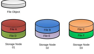
4.3.1 Simple File Distribution . . . 57

4.3.2 File Striping . . . 58

4.3.3 File Replication . . . 59

4.4 Parallel Virtual File System (PVFS) . . . 61

4.4.1 Background . . . 61

4.4.2 Architecture . . . 61

4.4.3 Distribution Techniques . . . 62

4.4.4 Feature Summary . . . 62

4.4.5 Performance Characteristics . . . 63

4.5 Lustre . . . 66

(11)

4.6 GlusterFS . . . 74

4.7 Hadoop Distributed File System (HDFS) . . . 83

5 IDENTIFYING APPLICATION PERFORMANCE CONSTRAINTS USING I/O PROFILES . . . 93

5.1 Introduction . . . 93

5.2 Establish an I/O Performance Baseline . . . 96

5.2.1 Set up the Environment . . . 96

5.2.2 Benchmark the Environment . . . 97

5.3 Generate an I/O Profile for an Application . . . 104

(12)

5.3.2 Profile of an I/O-Bound Application . . . 105

5.4 Case Study: seqprocessor . . . 109

5.5 Summary ofseqprocessor Performance Improvements . . . 115

5.6 Tuning Application I/O Operations . . . 116

5.7 Profiling Random I/O Applications . . . 118

5.8 Profiling Parallel I/O Applications . . . 120

5.9 Wrapping It Up . . . 121

6 CONCLUSION . . . 122

6.1 Wrapping It Up . . . 122

6.2 Extensions of This Research . . . 123

6.2.1 Parallel File Transfer . . . 123

6.2.2 Data Management: Storage Zones and Data Preservation Strate-gies . . . 124

6.2.3 Statistical Model to Calculate the Ideal Number of Hot-Swap Disks to Include in a Storage System . . . 125

6.2.4 Disaster Recovery of Parallel Distributed File Systems . . . 125

6.2.5 Persistent Versus Non-Persistent Scratch Space in HPC Envi-ronments . . . 126

6.2.6 Objective-C Inspired Dynamically Generated Non-Persistent Scratch Space for HPC Environments . . . 127

6.2.7 Extended Application I/O Profiling . . . 129

BIBLIOGRAPHY . . . 131

(13)

B DATA CLASSIFICATION . . . 139

B.1 Large Multimedia Files (Greater Than 100MB) . . . 139

B.2 Large Text Files (Greater Than 100MB) . . . 140

B.3 Large Compressed Files (Greater Than 100MB) . . . 140

B.4 Large Database Files (Greater Than 100MB) . . . 141

B.5 Medium Multimedia Files (1MB - 100MB) . . . 141

B.6 Medium Text Files (1MB - 100MB) . . . 142

B.7 Medium Compressed Files (1MB - 100MB) . . . 142

B.8 Medium Database Files (1MB - 100MB) . . . 143

B.9 Small Files (Less Than 1MB ) . . . 143

B.10 Large Number of Files (Small or Large) . . . 144

C APPLICATION I/O PROFILING WORKSHEET . . . 145

D ATLANTIS RESEARCH CLUSTER CONFIGURATION . . . 147

D.1 Storage Node Specifications . . . 147

D.2 Network Diagram . . . 148

D.3 Chapter 4 RAID Configuration and Performance Baseline . . . 148

D.4 Chapter 5 RAID Configuration and Performance Baseline . . . 149

E SEQPROCESSOR APPLICATION SOURCE CODE . . . 152

E.1 Seqprocessor Version 1 . . . 152

(14)

2.1 Storage zone policy definitions . . . 15

3.1 Probability of disk failure based upon SMART data [34] . . . 26

3.2 Comparison of desktop, nearline, and enterprise disk drive classes . . . 32

3.3 Description of commonly used RAID levels . . . 37

4.1 Summary of PVFS design features . . . 62

4.2 Summary of PVFS configuration on Atlantis . . . 63

4.3 Summary of Lustre design features . . . 69

4.4 Summary of Lustre configuration on Atlantis . . . 70

4.5 Summary of GlusterFS design features . . . 76

4.6 Summary of GlusterFS configuration on Atlantis . . . 77

4.7 Summary of HDFS design features . . . 86

4.8 Summary of HDFS configuration on Atlantis . . . 88

4.9 Summary of HDFS configuration on GeneSIS . . . 88

5.1 Tools for benchmarking disk subsystems and network interconnects . . . 98

5.2 Bonnie++ throughput results for md0 on atlantis01 . . . 102

5.3 Bonnie++ IOPS results for md0 on atlantis01. . . 102

5.4 Tools for monitoring system utilization . . . 104

5.5 Summary ofseqprocessor performance improvements . . . 117

(15)

D.2 Chapter 4 throughput results for md0 on atlantis00 . . . 149

D.7 Chapter 5 IOPS results for md0 on atlantis01 . . . 151

(16)

1.1 Anatomy of a high-performance storage system . . . 2

2.1 Native file system client communicating directly with storage nodes over a dedicated private interconnect such as Infiniband . . . 12

2.2 CIFS/NFS client communicating with a storage gateway over a

work-station network such as gigabit Ethernet . . . 12 2.3 Digital pictures are downloaded from a camera to storage zone A via

USB . . . 15

2.4 Video content is downloaded from a video camera to storage zone B

via Firewire . . . 16 2.5 Digital pictures are touched up and stored back in storage zone A . . . . 16 2.6 Movie is rendered from source material in zones A and B and written

to zone C . . . 16 2.7 Hi-def version is compressed and written to zone B . . . 16 2.8 Hi-def version is written to Blu-ray disks . . . 17 2.9 Intermediate movie files in zone C are removed from the storage system 17

3.1 Bathtub curve representing disk failure rates [56] . . . 25 3.2 Diagram of the various layers in the storage stack . . . 30 3.3 Probability of encountering an Unrecoverable Read Error while

rebuild-ing an array of n+1 disk drives . . . 39

(17)

4.1 Example of “parallel” distributed file system architecture . . . 56

4.2 Simple file distribution technique . . . 57

4.3 File striping distribution technique . . . 58

4.4 File replication distribution technique . . . 60

4.5 PVFS basic file transfer with file striping (64KB) . . . 64

4.6 PVFS block-range file transfer with file striping (64KB) . . . 64

4.7 PVFS client scalability with file striping (64KB) . . . 66

4.8 Lustre basic file transfer with simple file distribution . . . 70

4.9 Lustre block-range file transfer with simple file distribution . . . 71

4.10 Lustre client scalability with simple file distribution . . . 72

4.11 Lustre client scalability with file striping (1MB) . . . 73

4.12 GlusterFS basic file transfer using various distribution techniques . . . 78

4.13 GlusterFS block-range file transfer using various distribution techniques 80 4.14 GlusterFS client scalability with simple distribution configuration . . . . 81

4.15 GlusterFS client scalability with 3x replication configuration . . . 82

4.16 GlusterFS client scalability with 128KB stripe configuration . . . 83

4.17 HDFS basic file transfer with 64MB blocks and 2x replication . . . 88

4.18 HDFS block-range file transfer with 64MB blocks and 2x replication . . 89

5.1 Iozone test using 4KB to 16MB block sizes on files up to 4GB . . . 99

5.2 Iozone test using 64KB to 16MB block sizes on files up to 32GB . . . 101

5.3 NetPIPE throughput results over GigE link with the default MTU of 1500 bytes . . . 103

5.4 I/O profile of dd reading a 32GB file using 1MB blocks . . . 106

(18)

5.6 I/O profile of dd writing a 32GB file using 1MB blocks . . . 107

5.7 topoutput from the dd(write) command . . . 108

5.8 topoutput from seqprocessor-1 application . . . 110

5.9 iostat output from seqprocessor-1 application . . . 111

5.10 I/O profile of seqprocessor-1 with a single disk subsystem for both read and write operations . . . 112

5.11 I/O profile of seqprocessor-2 with a single disk subsystem for both read and write operations . . . 113

5.12 I/O profile of seqprocessor-2 with separate disk subsystems for read and write operations . . . 114

5.13 topoutput from seqprocessor-2 application with separate disk sub-systems for read and write operations . . . 115

5.14 I/O profile of seqprocessor-3 with separate disk subsystems for read and write operations . . . 116

D.1 Network layout of Atlantis research cluster . . . 148

(19)

HPC – High-Performance Computing

IOPS – Input/Output Operations Per Second

SMART – Self-Monitoring, Analysis, and Reporting Technology

DFS – Distributed File System

ROMIO – A High-Performance, Portable MPI-IO Implementation

GigE – Gigabit Ethernet

10GigE – 10 Gigabit Ethernet

IPoIB – IP network protocol transported over Infiniband datalink protocol

(20)

CHAPTER 1 INTRODUCTION

1.1 Background

The Mercury project was started in October 1958, and fewer than 4 years later NASA had placed John Glenn in orbit around the earth. The level of planning and technological achievement required to make that happen was phenomenal. Now, 52 years later, we owe much of our modern technology to these efforts. During the Mercury project, multiple IBM 709 computer systems were used to assist in the data processing effort [31]. The IBM 709 was capable of up to 12 kiloflops or 12,000 floating-point operations per second [25]. In comparison, the Intel i7 processor in my personal desktop system is capable of 40 gigaflops or 40,000,000,000 floating-point operations per second [26].

(21)

Many issues are involved in the design and construction of these high-performance

storage systems. Individuals looking to deploy such a system must make design

decisions based upon requirements for throughput, latency, redundancy, availability, capacity, scalability, number of processing clients, power, and cooling. The diagram in Figure 1.1 gives a high-level look at the different components that must be considered in the design of a high-performance storage system.

Customer’s Application

Storage Node

Disk Subsystem

CPU

Memory

Storage Node

Disk Subsystem

CPU

Memory

Storage Node

Disk Subsystem

CPU

Memory

Storage Node

Disk Subsystem

CPU

Memory

Network Interconnect Distributed File System

Processing Nodes

(22)

1.2 Commercial Storage Solutions

There are a number of options to consider when looking to deploy a high-performance storage system. Will it be a home-grown system with custom-built hardware and open source software? Or will it be a commercial, turn-key solution with proprietary software? Two popular proprietary options are provided by Panasas and OneFS. The underlying questions of hardware selection, disk subsystem reliability, and distributed file system selection are addressed by engineers from the respective companies. There are also commercial, open source, options provided by Penguin Computing and Microway that allow for customized storage solutions but that are still essentially turn-key.

Regardless of who provides the storage solution, it is important to understand how it will be used to ensure that it is configured properly. These include issues of usable capacity, redundancy of data, throughput and latency, as well as how data will flow through the system and be archived. Additional criteria include whether an organization has adequate facilities with space, cooling, and power. There may also be policies or contract requirements for vendors to provide maintenance agreements with specific service levels, such as having a technician on-site within four hours.

A vendor’s sales engineer may be able to assist with answering these questions, but they are trying to selltheir solution, not necessarily the best solution. Understanding the requirements of a storage system up front can save a lot of frustration later on.

1.3 Problem Statement

High-performance storage systems are complicated, requiring expert-level knowledge

(23)

storage system design is incomplete and scattered across a number of sources. In addition, the knowledge that comes from the experience of working directly with these systems is localized within corporations and national laboratories and not generally available except in mailing lists and user forums.

This thesis addresses four areas in storage system design. Each of these areas was a pain point during the construction and maintenance of GeneSIS, a Beowulf style Linux cluster with 84TB of storage located in the HPC lab at Boise State University, requiring months of research and experimentation to understand and incorporate back into the design of GeneSIS. Each of the following questions addresses one of these areas.

1. What questions should be asked when determining storage system design re-quirements?

2. What techniques for designing disk subsystems best protect data against latent sector errors and infant disk mortality?

3. Which distributed file system will best meet the performance and scalability requirements of the storage system?

4. How can I determine the performance constraints and I/O characteristics of a given application?

(24)

research papers, user guides, mailing lists, SC2009 conference presentations, and the lessons learned from the design and maintenance of GeneSIS. The above questions are not specific to GeneSIS and are not entirely unique to high-performance storage system design. As a result, the information provided in this thesis will be valuable long after the current technology has been consigned to the scrap heap.

1.4 Thesis Overview

There is a lot more to designing a storage system than simply purchasing a bunch of cheap, fast disks, putting them in servers, and installing some open source software. Chapter 2 discusses the questions to answer when designing a storage system. It is presented from the perspective of a storage consultant designing a storage system for a customer, but in reality the information presented applies to anyone considering the deployment of a high-performance storage system.

Storage systems are made up of hundreds or thousands of disks grouped together by RAID or some other mechanism into disk subsystems and these disk subsystems are the building blocks for a reliable, high-performance storage system. Chapter 3 takes a close look at how to design reliable disk subsystems in the presence of the well-published issues of latent sector errors and infant disk mortality.

(25)

(26)

CHAPTER 2 UNDERSTANDING STORAGE SYSTEM

REQUIREMENTS

2.1 Overview

Before disk drives and RAID volumes, before interconnects and file systems, before thinking about tower vs rack cases, a storage engineer must carefully consider the system requirements when designing a new storage system. In the words of Sherlock Holmes, “It is a capital mistake to theorize before one has data. Insensibly one begins to twist facts to suit theories, instead of theories to suit facts.” [5] This quote, taken from “A Scandal in Bohemia,” applies remarkably well to storage engineering. Invest time in gathering the facts, then design a storage system to fit the facts. Remember, the storage engineer’s job is to help the customer solve a problem, not create a new one.

(27)

with to design and build a bridge across a river. He spends two years on the project, and when he is finished he has constructed a beautiful foot bridge, complete with solar-powered LED lighting system and dedicated bike lanes. When the customer returns to inspect the work, he is shocked. How is he supposed to join two six-lane freeways together with a simple foot bridge?

In the bridge example, the customer knows his needs: type of traffic, number of lanes, weight requirements, etc. These are physical. In the early design phases, the customer would see the plans that the engineer was drafting and realize, before construction began, that the foot bridge would not meet his needs. The requirements for storage systems, on the other hand, are more abstract, making it difficult for customers to know their needs. The customer typically understands the problem he is trying to solve but not what it will take to solve it. This is where the storage engineer must be a good listener and part psychic. Helping the customer probe these issues enables the storage engineer to design a storage system that will meet the customer’s needs without excessive cost and complexity.

(28)

2.2 Background

Why is the customer considering a high-performance storage system? This is a good opportunity to learn about the particular problems the customer is attempting to solve. Chances are that there is an existing storage solution in place, either in a production or a development environment. What aspects of the existing solution are currently meeting the customer’s needs? What are the actual and perceived limitations of the existing solution?

Managers, application developers, and system engineers can have drastically dif-ferent concerns from a storage perspective. Managers are concerned with maintenance cost and return on investment. Managers like fixed, known costs and they care about the big picture. Application developers want to quickly store and retrieve data in the form of streams, objects, or flat files. Application developers like simple, configurable interfaces for I/O operations. Application developers resist changing code to improve performance, preferring to push for faster hardware. System engineers care about ease of management, scalability, performance, backups, data integrity, disaster recovery, and maintenance agreements. If the managers, application developers, and end-users are happy, then the system engineer is happy.

2.3 Storage Capacity and Growth

(29)

usable capacity for his application. After considering the critical nature of the data, it is decided that 2x replication should be used at the file system level and RAID10 should be used at the disk level; the resulting raw capacity requirements are in fact 80TB.

Another aspect of storing data is how quickly the data will grow. How much storage capacity will be required over the next two to three years? This is a difficult question to answer, but it is important to consider as it affects many of the storage system design decisions. Planning for growth often increases the initial system cost but can significantly decrease the cost to scale the system, especially in installations where floor space / rack space comes at a premium.

(30)

be a bargain when it comes time to expand the capacity of the storage system.

Another benefit of designing a system for scalable growth is that it leverages the trend for decreasing hardware costs over time. An example of how this trend can be leveraged is by purchasing raw disk capacity to meet the customer’s initial storage needs plus 20% extra for growth. Several months later, as the customer’s storage needs increase and the price of disk storage has dropped, the storage capacity can be increased by purchasing additional (and possibly larger) storage disks. The idea for this approach is that the customer is not paying a premium for storage that is not needed yet. This strategy can be modified to account for the growth rate of the customer’s data as well as the customer’s policies for disk drive replacement.

An important item to consider when planning for growth is vendor support for hardware upgrades. Our research lab purchased an EMC AX150 in 2007, configured with twelve 500GB SATA disk drives. In 2010, we wanted to upgrade this unit with 1TB SATA disk drives, but EMC customer support stated that the unit would only support up to 750GB capacity disk drives. To top it off, only hard drives purchased directly from EMC would work in the unit, and those drives cost six times more than retail. This was a limitation enforced in the device firmware, and the solution recommended by EMC customer support was to purchase the latest model of chassis.

2.4 Storage Client Details

(31)

shared disk and parallel distributed file systems are developed specifically for Linux environments. Several of these file systems have native clients that work on MacOS and Unix, but not Windows. Connecting a Windows client requires the use of a gateway node. Gateway nodes can be used as a cost-effective method of providing clients access to the storage system, but they can easily become a performance bottleneck. For that reason, it is preferable for client systems to use native file system clients.

High Performance Storage System Native

Storage Client

Figure 2.1: Native file system client communicating directly with storage nodes over a dedicated private interconnect such as Infiniband

High Performance Storage System Storage Client

Gateway CIFS/NFS

Storage Client

Figure 2.2: CIFS/NFS client communicating with a storage gateway over a worksta-tion network such as gigabit Ethernet

(32)

As the number of clients increases, the load on the storage system will increase. Increasing the aggregate throughput of the storage system requires either an upgrade to the storage interconnect, the addition of more storage nodes, or both. Knowing that the number of clients is going to increase can mean using an Infiniband interconnect, rather than gigabit Ethernet, to increase the throughput each storage node is able to provide. The local disk subsystems on the storage nodes will also need to be configured to supply data at the increased throughput levels.

2.5 Data Details

2.5.1 Data Classification

A good source of information for helping with storage system design decisions is the actual data that will be stored on the system. Quite often, data is thought of as simply information stored on hard disks and retrieved by various applications. However, a good understanding of the data can reveal a lot about how the storage system should be designed.

For instance, large video files are processed sequentially, either as a stream or in chunks. Video files typically support concurrent client access, which can lead to a performance bottleneck. Distributing a video file across multiple nodes using striping can improve performance. Because the files are processed sequentially, they can benefit from read-ahead caches, which can help hide interconnect and file system latency.

(33)

up to 128KB [47]. As a result, interconnect latency and file system overhead can severely limit the throughput performance.

Appendix B contains a general list of data classes and some of the characteristics of each. These classifications should not be used as firm, fixed rules, but rather as guidelines to help a storage engineer begin thinking about how the data can influence system design. In the end, it is the application that determines how the data is accessed, but looking at the type of data is a good place to start.

2.5.2 Storage Zones

It is a rare storage system that stores a single type of data. The result is that there are mixtures of large and small files. Some data types are primarily read-only while others are read-write. In addition, there are questions of data redundancy and backup, as well as performance requirements that may be different depending upon the type of data. Unfortunately, there is not a one-size-fits-all solution that will meet all of a customer’s data storage and processing requirements.

To address these issues in data management, storage zones can be defined to group data based upon type, client-access requirements, and data redundancy and backup policies. Storage zones can also have policies defined for data lifetime to prevent stale data from wasting space on the storage system. Multiple storage zones can be defined on a storage system. Storage zones are only guidelines for managing data on a storage system and are not enforced by the storage system.

(34)

the storage engineer understand the throughput requirements of each client. From the example, the clients transferring media to the storage system do not require 10 gigabit Infiniband interconnects since the throughput will be limited by the source devices. The clients processing the digital photos in Figure 2.5 also do not require high levels of throughput. For these clients, accessing a gateway node using CIFS or NFS over gigabit Ethernet will be more than sufficient. The clients in Figures 2.6 and 2.7 will be doing work that is CPU intensive. However, if the application is multithreaded and the client systems have a lot of processing power, clients performing these operations could benefit from a high throughput interconnect such as Infiniband.

Table 2.1: Storage zone policy definitions

Zone Name Throughput Data Distribution Backups

A Med Simple Nightly Full

B Med Striped Weekly Full with Nightly

Incremental

C High Striped None

Zone C Photos

(10 - 20 MB/s)

Zone B Zone A

Figure 2.3: Digital pictures are downloaded from a camera to storage zone A via USB

(35)

Zone C Video Content

(60 - 80 MB/s)

Zone B Zone A

Figure 2.4: Video content is downloaded from a video camera to storage zone B via Firewire

Zone C Zone B Zone A Photos

Edited Photos

Figure 2.5: Digital pictures are touched up and stored back in storage zone A

Zone C Zone B Zone A Photos

Video Content

Uncompressed Hi-Def Video (80 – 160MB/s)

Figure 2.6: Movie is rendered from source material in zones A and B and written to zone C

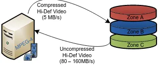
Zone C Zone B Zone A Compressed

Hi-Def Video (5 MB/s)

MPEG -4

Uncompressed Hi-Def Video (80 – 160MB/s)

Figure 2.7: Hi-def version is compressed and written to zone B

(36)

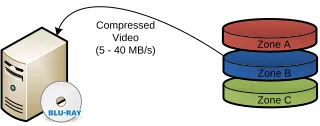
Zone C Zone B Zone A Compressed

Video (5 - 40 MB/s)

Figure 2.8: Hi-def version is written to Blu-ray disks

Zone C Zone B Zone A

Cleanup Intermediate Video Files

Figure 2.9: Intermediate movie files in zone C are removed from the storage system

system. Storage systems that are not managed effectively can quickly go from high performance systems to poor performing ones.

2.6 Applications Details

The data can give part of the picture, but achieving high performance for customer applications requires a solid understanding of the flow of data and of how the ap-plications interact with the storage system. To begin, the system engineer needs to have a list of applications that will interact with the storage system. This is where it is helpful to sit down with application developers, system engineers, and end-users. Discuss how they use the storage system, work out their process flows, and compose a list of applications. This is also a good chance to discuss performance issues.

(37)

Chapter 5 provides an in-depth discussion of tools that are available to assist with this process. These profiling techniques can identify whether an application is I/O bound, memory bound, or CPU bound. They can also provide information on the current read and write throughput as well as the percent read vs percent write operations. This information is useful because it can help the storage engineer understand the throughput requirements of an application, but it can also help gauge expectations of application performance. If an application is CPU bound, moving the data to the fastest storage system in the world will not improve the performance of the application. [47]

2.7 Disaster Recovery

Questions of uptime and high availability (HA) all relate to how much redundancy is built into the system. There are two different aspects to this topic. The first is data redundancy, focusing on replication and backups. The second is system availability, focusing on building levels of redundancy into the storage nodes and interconnect to ensure that the system can remain functional in the event of hardware failures.

In many cases, there is a trade-off between performance and redundancy. Most high performance parallel distributed file systems do not provide built-in functionality for HA or data replication; instead, they rely on the underlying systems to implement this functionality. File systems that do provide replication typically sacrifice some write performance. Understanding the customer’s need for performance vs redun-dancy is imperative when designing a storage system.

(38)

to allow the storage system to shut down cleanly or transition to backup power generators. Storage systems use several layers of caching to improve performance. To prevent loss of data, the write caches must be flushed to disk. Design the system so that data is not lost in the event that a single disk or even an entire storage node fails. Xin et al. writes in “Reliability Mechanisms for Very Large Storage Systems”: “Based on our data, we believe that two-way mirroring should be sufficient for most large storage systems. For those that need very high reliability, we recommend either three-way mirroring or mirroring combined with RAID” [57]. A high level of reliability for business critical data can be achieved using a layered approach. First, configure the RAID subsystem in the storage nodes to ensure that a single (or multiple) disk failure will not result in data loss. Second, replicate data across multiple storage nodes, ensuring that no data is lost in the event of a complete node failure. And of course, perform regular backups of critical data to external disks or tape.

Is access to the storage system critical to business operation? If so, the system should employ file replication or shared block devices with HA fail-over. There should also be redundant storage interconnects and any gateway nodes should be configured for HA. Storage nodes can be configured with dual power supplies, redundant memory, and even an internal Fibre Channel loop with dual controllers. The key here is to balance the level and expense of redundancy against the risk of failure and the cost of downtime.

2.8 Facility

(39)

as well as a fixed amount of power available in each rack. In co-location environments, maximize the amount of storage per rack while staying within the available power limits. A benefit of co-location facilities is that most provide site-wide UPS systems with automatic fail-over to backup generators in the event of power failure.

2.8.1 Power Requirements

If the system is installed at the customer’s site, ensure that the facilities have sufficient power and cooling. It would be unfortunate to design and build a beautiful four-rack storage system but only have a single 20amp circuit to power it. A rough estimate of the storage system power requirements can be obtained by examining the input voltage and amp requirements for each storage node. This can be found printed on a label on the back of the power supply or in the documentation included with the storage node. This number will be a max power level. To obtain a more “real-world” value, attach an amp meter to a storage node and run a series of tests to simulate peak load on CPU cores and disk drives. Assuming that all the storage nodes require the same input voltage, multiply both the max amps and the real-world amps by the number of storage nodes. The result is the max and real-world amperage requirements for the storage system at the required input voltage.

The power required for the storage nodes will dominate the overall power require-ments of the storage system, but it is a good idea to check the power requirerequire-ments of interconnect devices (switches, routers, etc.) as well as plan for growth of the storage system. These values for max and real-world amperage can be used to calculate VA and Watt values for UPS specification. Remember to plan for power for the cooling system as well.

(40)

Watts = voltage * amperage * pf

Sizing a UPS system is not a trivial task. An important fact that many people overlook is that UPS systems have ratings for capacity in terms of Volt-Amps(VA) and Watts. Volt-Amps are used to measure the “apparent” power usages while Watts measure the actual power usage [35]. Volt-Amp capacity measurements are used for marketing, but the nasty little secret in the UPS industry is that many UPS systems have a power factor(pf) as low as 0.66 [2]. This means that a 1000VA UPS system will only be able to power a load of 660 watts. Unlike UPS manufactures, who often calculate wattage capacity assuming a power factor in the range of 0.66 to 0.90, most modern computer systems have a power factor approaching 1.0 (unity) [2]. Many UPS manufactures provide capacity planning tools to match UPS systems to site-specific load and run-time requirements.

2.8.2 Cooling Requirements

An estimate of the cooling requirements for the storage system can be calculated from the above power requirements. Due to the fact that essentially all of the power consumed by the storage system is converted to heat, the thermal output of the storage system is the same as the power input [36]. Heat generated by the storage system is equivalent to the max and real-world wattage values calculated above. These values can be converted to BTUs or Tons using the following formulas: [36].

BTU per Hour = 3.41 * Watts Tons = 0.000283 * Watts

(41)

must consider all the possible heat sources. These include IT Equipment, UPS with Battery, Power Distribution, Lighting, and People [36]. In addition, care must be taken in planning for growth of the storage system. It is strongly recommended to consult with an HVAC engineer experienced with data-center cooling systems once the power requirements have been identified.

2.9 Budget

The customer’s budget is the single most influential factor in the storage system design. Sections 2.1 through 2.8 deal with identifying what the customer needs from the storage system design. The budget determines what the customer can afford to buy. Ideally, the customer can afford what he or she needs, but too often this is not the case. In such an event, compromise becomes the order of the day. High-capacity, high-performance, high-reliability, and low cost lie in the four corners of the magic square of storage system design, unfortunately storage engineers can only choose up to three of these to include as priorities in the storage system design.

(42)

When a component in a storage system fails, the time required to replace the failed component is referred to as the window of vulnerability. A large window of vulnerability increases the probability of data loss, so it is critical to have processes

in place to quickly replace failed components [57]. To minimize the window of

vulnerability, budget for spare components or purchase a maintenance agreement with four-hour or next-day on-site service.

Finally, budget time for an engineer to maintain the storage system. A storage system will require monitoring to detect potential issues as well as someone to replace components when they fail. Components will fail. “In petabyte-scale file systems, disk failures will be a daily (if not more frequently) occurrence” [57]. The amount of time to budget for an engineer will vary depending upon the size of the storage system.

2.10 Conclusion

(43)

CHAPTER 3 DESIGNING RELIABLE DISK SUBSYSTEMS IN THE

PRESENCE OF LATENT SECTOR ERRORS AND

INFANT DISK MORTALITY

3.1 The Threat to Disk Subsystems

It is easy to assume that when a file is stored to disk it will be available and unchanged at any point in the future. However, this is not guaranteed. Imagine a world where disk manufacturers publish expected bit error rates of one in every 12TB read, where large numbers of disks fail in their first year of operation, and where data can be silently altered between the computer’s memory and the hard disk platters. This world is in fact our reality. This chapter will examine the issues of infant disk mortality, latent sector errors, and silent data corruption, and provide recommendations for how to configure reliable disk subsystems to protect against these issues.

3.1.1 Infant Disk Mortality

(44)

deployments indicate that disk drives are replaced by a factor of 2 - 10 times the rate suggested by the MTBF rating [37, 22, 58]. That fact alone is concerning, but these studies have also shown the shape of the drive failure curve to be bathtub shaped with the bulk of the failures coming in the first year of operation or at the end of the life of the drive (typically 5 years) [58].

Decreasing Failure

Rate

Constant Failure

Rate

Increasing Failure

Rate

F

a

il

u

re

R

a

te

Wear Out Failures Early

"Infant Mortality" Failure

Constant (Random) Failures Observed Failure

Rate

Time

Figure 3.1: Bathtub curve representing disk failure rates [56]

(45)

failures were random and evenly distributed across the expected life of the drive. The Observed Failure curve depicts the bathtub shaped failure curve discussed previously.

Table 3.1: Probability of disk failure based upon SMART data [34]

SMART Counter

Probability of fail-ure within 60 days

Description

Scan Errors: 39 times more

likely to fail

Sometimes referred to as seek errors, these errors occur when the drive heads are not properly aligned with the track. Reallocation

Count:

14 times more

likely to fail

The number of sectors that have failed and been remapped.

Offline

Re-allocation Count:

21 times more

likely to fail

The number of failed sectors that were detected and remapped using back-ground disk scrubbing.

Probational Count:

16 times more

likely to fail

The number of sectors that experienced read errors and that rescheduled to be remapped upon the next write oper-ation unless a successful read of the sector occurs before the remap.

Modern disk drives provide extensive monitoring capabilities through a standard-ized interface called SMART (Self-Monitoring, Analysis, and Reporting Technology). Several attempts have been made to accurately predict when a disk drive is about to fail by using this SMART data. A study examining a large collection of disk drive failure and usage information gathered by Google attempted to ascertain whether

SMART counters can be used to predict drive failure. This work showed that

(46)

these values would have been significantly higher if not for the initial system burn-in testing that disks go through before being put into production. Table 3.1 shows some interesting statistics from this study. Other items of interest are that drive activity and temperature do not have a significant impact on drive failures [34].

3.1.2 Latent Sector Errors

A latent sector error is a generic term that is used when a disk drive is unable

to successfully read a disk sector. Latent sector errors can show themselves as

Sector Errors, Read Errors, Not-Ready-Condition Errors, or Recovered Errors. They can be caused by a variety of factors including media imperfections, loose particles causing media scratches, “high-fly” writes leading to incorrect bit patterns on the media, rotational vibration, and off-track reads or writes [3]. The term bit error rate (BER) refers to the frequency that unrecoverable/uncorrectable read errors (URE) are expected to occur. Manufacturers publish expected bit error rates based upon disk drive class (see Section 3.2.1 for definition of desktop, nearline and enterprise disk classes). These errors are considered part of normal disk operation as long as the errors are within the rate provided in the disk specification. The dirty little secret about latent sector errors is that they are only detected when an attempt is made to read the sector. This means that a disk may contain corrupted data without the user knowing it.

Schwarz et al. observed that latent sector error rates are five times higher than disk failure rates [38]. As a result, latent sector errors can wreak havoc on RAID

arrays. For example, imagine a 2TB array with three 1TB disks in a RAID-5

(47)

regenerating the RAID striping on the new disk from the remaining two disks. Three quarters of the way through the rebuild process, one of the disks from the original array encounters an unrecoverable read error. At this point, the RAID set is lost and the data can only be retrieved using time consuming and expensive data recovery techniques.

Microsoft Research conducted a study focused on the bit error rates advertised by disk manufacturers. They performed a series of tests where they would generate a 10GB file and calculate the checksum. Then, they would read the file and compare the checksum of the file to the original checksum to test for read errors. The results were written to disk, then the test was repeated. This was run for several months with a total of 1.3PB of data transferred. Another round of tests was performed using 100GB test files and continually reading the file to test for bit-rot. These tests moved more than 2PB of data and read 1.4PB. They observed a total of four definite uncorrectable bit errors and one possible uncorrectable bit error across all of their tests. However, in their testing they saw far more failures in drive controllers and operating system bugs than in read errors. Their conclusion is that bit error rate is not a dominant source of system failure [22]. However, their testing was conducted across four test systems with a combined total of only seventeen hard disk drives. This is a statistically insignificant number of disks. Other studies by Bairavasundaram et al. and Pˆaris et al. demonstrate that bit error rates and latent sector errors can have a significant impact on storage system reliability [4, 3, 32].

(48)

the disk when that sector was written. An interesting finding from this study is that nearline class disks develop checksum errors at a rate that is an order of magnitude higher than enterprise class disks (see Section 3.2.1 for definition of desktop, nearline and enterprise disk classes). This study also provides a section on “Lessons Learned” including recommendations for aggressive disk scrubbing, using staggered stripes for RAID volumes, and replacing enterprise class disks at the first sign of corruption [4].

In the literature, several ideas have been put forward as techniques to help ad-dress the issues of latent sector errors. These include a variety of intra-disk parity schemes [13], using staggered striping for RAID volumes [4], and a variety of disk, file/object, and RAID scrubbing techniques [3, 4, 32, 38]. Unfortunately, many of these ideas are not generally available for use in production environments. However, Mean Time To Data Loss (MTTDL) models that account for latent sector errors, RAID scrubbing has been shown to increase reliability by as much as 900% [32].

3.1.3 Silent Data Corruption

Silent data corruption can occur in processor caches, main memory, the RAID con-troller, drive cables, in the drive as data is being written, or in the drive as the data is being read. Desktop and workstation class systems with standard DDR3 memory and SATA disk drives are far more susceptible to silent data corruption than enterprise class systems (enterprise class servers have error correcting memory, high end RAID controllers with built-in error correcting procedures, SCSI, SAS, and FC protocols that natively support error correction, and enterprise class disk drives with an extra eight bytes per sector to use for storing checksum data directly on the disk.)

(49)

the lower levels represent the physical storage hardware. Data corruption can occur at any of these layers. Even with enterprise class hardware, errors introduced at a high level in the storage stack will be silently stored to disk.

Application System Libraries

Virtual File System Kernel Interface

(VFS) Disk File System Processors and Memory Storage Controller Disk Controller Backplane and Cables Disk Platters F lo w o f s to re d d a ta F lo w o f s to re d d a ta F lo w o f r e tr ie v e d d a ta F lo w o f r e tr ie v e d d a ta Device Drivers Device Drivers Upper Layers Lower Layers

Figure 3.2: Diagram of the various layers in the storage stack

(50)

3.2 Disk Considerations

Disks drives are the building blocks of a disk subsystem. Understanding the char-acteristics of the various types of rotational storage media will go a long way for designing a reliable disk subsystem.

3.2.1 Classes of Disks

There are a wide variety of disk drives available on the market with an equally wide variety of performance, capacity, and error correction features. These disks have been loosely categorized into classes based upon a particular feature set. Originally, there were two basic classes: desktop and enterprise. Desktop drives used the ATA interface protocol while enterprise class disks used the SCSI protocol. In recent years, the distinction between desktop and enterprise class disks has blurred. The development of aggressive power management and data recovery features as well as the fact that disk drive classifications are not consistent across manufacturers makes choosing the appropriate disks for a storage system a challenge.

(51)

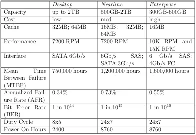
nearline and enterprise disk classifications used in the papers and articles cited in this thesis. Table 3.2 is derived from several white papers published by Seagate to show the differences between the different disk classes [43, 42, 40, 41, 39].

Table 3.2: Comparison of desktop, nearline, and enterprise disk drive classes

Desktop Nearline Enterprise

Capacity up to 2TB 500GB-2TB 300GB-600GB

Cost low med high

Cache 32MB; 64MB 16MB; 32MB;

64MB

16MB

Performance 7200 RPM 7200 RPM 10K RPM and

15K RPM

Interface SATA 6Gb/s 6Gb/s SAS;

SATA 3Gb/s

6 Gb/s SAS;

4Gb/s FC

Mean Time

Between Failure (MTBF)

750,000 hours 1,200,000 hours 1,600,000 hours

Annualized Fail-ure Rate (AFR)

0.34% 0.73% 0.55%

Bit Error Rate (BER)

1 in 1014 _{1 in 10}15 _{1 in 10}16

Duty Cycle 8x5 24x7 24x7

Power On Hours 2400 8760 8760

3.2.1.1 Desktop Class

(52)

slow responding while waiting for the disk to speed up. In the worst case, the RAID controller will assume the drive has failed and drop it from the array. Depending upon the number of drives and the type of RAID subsystem, it is possible, even likely, that multiple drives will enter power-save mode and be dropped from the RAID set. The RAID array will then be degraded and must be recovered, possibly resulting in data loss.

The second feature of desktop drives that makes them unsuitable for RAID en-vironments is that they have some extremely powerful sector recovery features built into the on-disk controller. At first glance, this might not seem like a bad thing, but this deep recovery cycle can be time consuming [27].

“When an error is found on a desktop edition hard drive, the drive will enter into a deep recovery cycle to attempt to repair the error, recover the data from the problematic area, and then reallocate a dedicated area to replace the problematic area. This process can take up to two minutes depending on the severity of the issue. Most RAID controllers allow a very short amount of time for a hard drive to recover from an error. If a hard drive takes too long to complete this process, the drive will be dropped from the RAID array. Most RAID controllers allow from seven to fifteen seconds for error recovery before dropping a hard drive from an array. Western Digital does not recommend installing desktop edition hard drives in an enterprise environment (on a RAID controller).” –Western digital FAQ [46]

(53)

Digital), Error Recovery Control (Seagate), and Command completion Time Limit (Samsung, Hitachi).

3.2.1.2 Nearline Class

There is not a consistent name for this class of hard drives across all manufacturers. A few examples of drives that fall into the nearline class include business class disks, low-cost server disks, enterprise class SATA, and nearline SAS. The performance and reliability features also vary widely between manufacturers and disk models. In some cases, the only difference between a manufacturer’s desktop and nearline class disk drives is the firmware on the drive controller.

In several of the papers cited in this thesis, the nearline disks have a bit error rate of 1 in 1014_{; however, in Table 3.2, nearline disks are shown with a bit error rate of 1}

in 1015. This discrepancy is due to the fact that the data in Table 3.2 is from 2011 and the disk drives in the cited studies are considerably older. In addition, the data in Table 3.2 is provided by Seagate; other disk manufacturers may have a higher bit error rate for their nearline class disk drives.

(54)

Nearline class disk drives are designed for use in RAID applications and are extremely well suited for large parallel distributed storage systems used in HPC environments. These environments often deal with 10s or 100s of TBs of data that require high levels of throughput, but not necessarily high numbers of IOPs, and the $/GB price point of nearline class disk drives is very attractive.

3.2.1.3 Enterprise Class

There are a number of key differences between desktop/nearline class disk drives and enterprise class disk drives. Enterprise class hard drives have a more rugged construction than desktop or nearline class drives that allows them to operate relia-bility in 24x7 data center environments with a continuous duty cycle. Desktop and nearline class disks have a fixed sector size of 512 bytes while enterprise class disks support variable sector sizes with the default being 520 to 528 bytes. These extra eight to sixteen bytes are leveraged for end-to-end data integrity to detect silent data corruption [27]. They also include specialized circuitry that detects rotational vibration caused by system fans and other disk drives and compensates by adjusting the head position on-the-fly to prevent misaligned reads and writes [27].

(55)

subsystem [38, 4, 32]. Section 3.4.3 discusses data scrubbing in greater detail with an example of usage in a production environment.

In addition, disk manufacturers implement a number of proprietary techniques to further increase the reliability of enterprise class disk drives. These efforts allow enterprise class disk drives to operate at twice the RPM of desktop and nearline class drives but still maintain a bit error rate that is two orders of magnitude lower than desktop class disks. The result is a trade-off of price and capacity for performance and reliability.

3.3 RAID Considerations

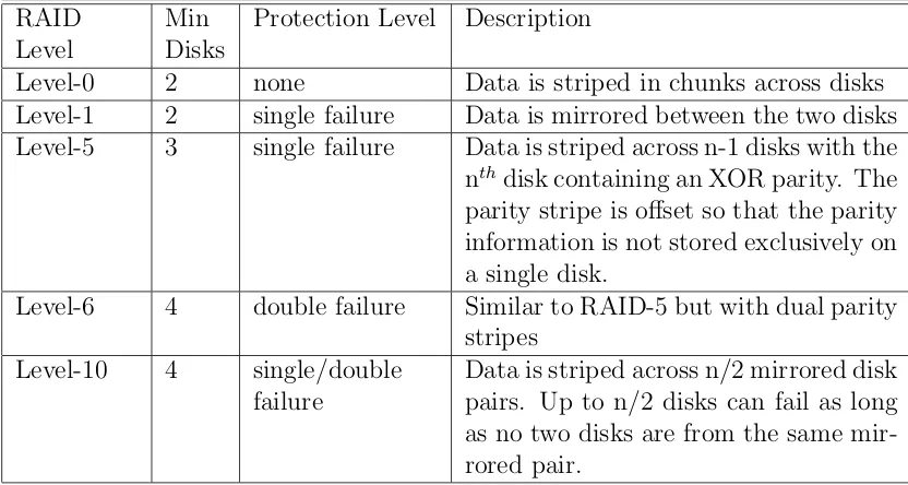
RAID is a powerful tool that can be leveraged to improve both the reliability and the performance of a disk subsystem. Xin et al. demonstrate that using the MTBF rates published by disk manufacturers, a 2PB storage system composed of 500GB nearline disks can expect to have one disk failure a day [57]. Add to this fact that many real-world studies conclude that actual disk failure rates are up to ten times higher than the manufacturer’s rates [32, 37, 22] and the need for RAID becomes apparent. Table 3.3 is a summary of the commonly used RAID levels in production environments.

(56)

Another way to think about this is with an analogy of soldiers protecting maidens. In a RAID-1 scheme, each soldier is charged with protecting a single maiden with his life. In a RAID-10 scheme, there are M pairs of soldiers and maidens with each soldier charged with protecting a single maiden (similar to RAID-1). In this scheme, any or all of the soldiers can die as long as the maidens remain unharmed; however, if a single maiden dies, it does not matter how many soldiers remain, the battle is lost. With RAID-5, a single soldier is charged with protecting N maidens with his life. And finally a RAID-6 scheme charges two soldiers with the responsibility of protecting N maidens. It is easy to understand that if a maiden has her own personal bodyguard, she is a lot safer when trouble comes knocking than the maidens who share protectors.

Table 3.3: Description of commonly used RAID levels

RAID Level

Min Disks

Protection Level Description

Level-0 2 none Data is striped in chunks across disks

Level-1 2 single failure Data is mirrored between the two disks

Level-5 3 single failure Data is striped across n-1 disks with the

nth_{disk containing an XOR parity. The} parity stripe is offset so that the parity information is not stored exclusively on a single disk.

Level-6 4 double failure Similar to RAID-5 but with dual parity

stripes

Level-10 4 single/double

failure

(57)

3.3.1 Encountering Latent Sector Errors

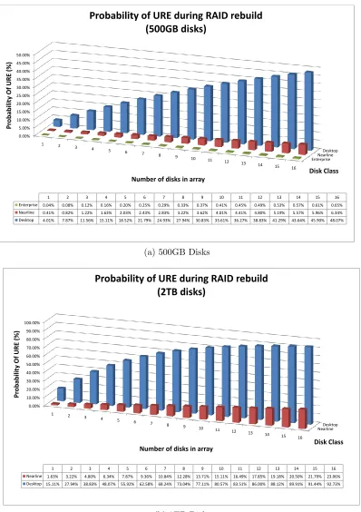
Care should be taken in the selection of the RAID level used as well as the number of disks in each RAID set. Pˆaris et al. conducted a study that looked specifically at RAID-1, RAID-5, and RAID-6 arrays in the presence of latent sector errors. The results indicate that unrecoverable read errors can reduce the mean time to data loss (MTTDL) of each of the three array types by up to 99% [32].

Figure 3.3 shows the probability of encountering an unrecoverable read error (latent sector error) while rebuilding an array of n+1 disks. Probabilities are shown for both 500GB (Figure 3.3a) and 2TB (Figure 3.3b) disk drives. These probabilities are calculated directly from the manufacturer’s published bit error rates for desktop, nearline, and enterprise class disk drives using the probability equations published by Adaptec Storage Advisors [1]. Observe that the probability of encountering an unrecoverable read error (URE) increases as the size of the storage array increases, by increasing either the capacity of the disks or the number of disks. Also observe that the probability of an URE decreases by an order of magnitude with each increase in disk class (Desktop − > Nearline − > Enterprise). The adage “you get what you pay for” has never been more true than in storage system design.

(58)

EnterpriseNearline Desktop 0.00% 5.00% 10.00% 15.00% 20.00% 25.00% 30.00% 35.00% 40.00% 45.00% 50.00%

1 ₂

3 ₄

5 ₆

7 8 ₉

10 11 ₁₂

13 ₁₄

15 16

Disk Class Pr o b abil ity Of URE (%)

Number of disks in array

1 2 3 4 5 6 7 8 9 10 11 12 13 14 15 16

Enterprise 0.04% 0.08% 0.12% 0.16% 0.20% 0.25% 0.29% 0.33% 0.37% 0.41% 0.45% 0.49% 0.53% 0.57% 0.61% 0.65% Nearline 0.41% 0.82% 1.22% 1.63% 2.03% 2.43% 2.83% 3.22% 3.62% 4.01% 4.41% 4.80% 5.19% 5.57% 5.96% 6.34% Desktop 4.01% 7.87% 11.56% 15.11% 18.52% 21.79% 24.93% 27.94% 30.83% 33.61% 36.27% 38.83% 41.29% 43.64% 45.90% 48.07%

Probability of URE during RAID rebuild (500GB disks)

(a) 500GB Disks

NearlineDesktop 0.00% 10.00% 20.00% 30.00% 40.00% 50.00% 60.00% 70.00% 80.00% 90.00% 100.00%

1 2 ₃

4 5 ₆

7 ₈

9 10 ₁₁

12 ₁₃

14 15 ₁₆

Disk Class Pr o b abil ity Of URE (%)

Number of disks in array

1 2 3 4 5 6 7 8 9 10 11 12 13 14 15 16

Nearline 1.63% 3.22% 4.80% 6.34% 7.87% 9.36% 10.84% 12.28% 13.71% 15.11% 16.49% 17.85% 19.18% 20.50% 21.79% 23.06% Desktop 15.11% 27.94% 38.83% 48.07% 55.92% 62.58% 68.24% 73.04% 77.11% 80.57% 83.51% 86.00% 88.12% 89.91% 91.44% 92.73%

Probability of URE during RAID rebuild (2TB disks)

(b) 2TB Disks

(59)

level of reliability for modern disk subsystems.

3.3.2 Utilizing Mean Time to Data Loss (MTTDL)

Figure 3.3 only reveals part of the picture. To adequately compare the relative merits of each of the different RAID levels requires a measure called mean time to data loss (MTTDL). MTTDL is a measure used to evaluate the reliability of a disk subsystem. Unfortunately, the values returned by most MTTDL models are next to useless. What value is it if a disk array has a MTTDL of 100,000,000 years versus 1,000,000 years? The trouble with most MTTDL models is that they do not take into account latent sector errors and silent data corruption. In addition, it is assumed that failures are evenly distributed and independent, not accounting for infant disk mortality, manufacturing issues, or firmware glitches. Many studies have examined the issues with MTTDL and proposed a variety of solutions including the use of Markov chains, Poisson distribution, and even Monte Carlo-based approaches [16, 3, 13, 58].

In spite of this debate over the accuracy of MTTDL, it can still be utilized as a measure for evaluating the relative reliability of different RAID protection schemes. Figure 3.4 shows the failure rates for a variety of RAID levels. These values are calculated based upon a simple MTTDL model that utilizes the MTBF values pub-lished by disk manufactures. As a result, the values themselves are nearly worthless since they do not account for latent sector errors and infant disk mortality. However, there is some value if we look at them from the perspective that they are best case values. What we see is that replication-based protection schemes have significantly lower failure rates than parity-based schemes.

(60)

of the combination of a limited number of tolerated failures with the probability of encountering corrupt data during a rebuild. In a replication-based protection scheme such as RAID-1 or RAID-10, the maximum number of disks that will need to be successfully read for a single disk failure is one. From Figure 3.3b, the probability of encountering a latent sector error is 1.63%. Not only is the risk of encountering a latent sector lower, but the time the array remains in a degraded state is lower since less data must be read to rebuild the array. With a parity-based protection scheme such as RAID-5 or RAID-6 with n disks, n-1 disks must be successfully read to regenerate the array. This results in both a higher probability of encountering a latent sector error and a longer period of time that the array remains in a vulnerable state.

(61)

3.4 Designing a Reliable Disk Subsystem

The following sections describe techniques that can be leveraged to construct reliable disk subsystems.

3.4.1 Disk Burn-in

From the Google study on infant disk mortality, it was suggested that the rate of infant disk mortality they were seeing in their systems would be significantly higher if not for their initial burn-in of disks before placing them in the production environment [34]. Taking a cue from Google’s playbook, the following guidelines can be used to help limit the effects of infant disk mortality on a storage system.

The idea with a disk burn-in is that rather than discovering latent sector errors or infant disk mortality of a new hard disk in a production server, use a tool to read and write a series of patterns across the entire surface of the disk to identify issues up front. The nice feature of a test like this is that if a latent sector occurs, the controller on the disk will remap the sector the next time it is written to. After the test completes, the SMART data will show the number of sectors that have been remapped. The following process demonstrates a basic sanity test (burn-in) for a new hard drive.

• Verify that the SMART counters for pending and remapped sectors is zero

• Use the badblocks utility to write test patterns over the surface of the disks

• Verify that the SMART counters for pending and remapped sectors are still

(62)

The badblocks utility can be configured to perform multiple passes across the disk surface until there are no bad blocks detected or until the max number of passes is completed. In the event that bad blocks (latent sector errors) are found on the disk surface, there are a couple of different schools of thought. One is that the disk is bad and should be returned to the manufacturer. This is supported by the disk failure statistics shown in Table 3.1. Unfortunately, what a user considers a bad disk does not always match up with what the manufacturer considers a bad disk. The definition of a drive failure is not well defined [34]. Schroeder and Gibson cite a disk manufacturer that reported that 43% of returned drives passed the its in-house quality testing [37].

The other school of thought suggests that a nearline disk drive can still continue to function properly even with a few remapped sectors as long as the counts do not continue to increase; however, enterprise class drives should be replaced at the first sign of latent sectors. This school of thought is supported by statistics gathered by Bairavasundaram in a study of 1.53 million nearline and enterprise class disk drives [4].

3.4.2 Leveraging RAID

(63)

An internal white paper published by Oracle introduced a new methodology called SAME [30]. SAME stands for Stripe and Mirror Everything. SAME has four basic rules:

1. Stripe all files across all disks using a one megabyte stripe width

2. Mirror data for high availability

3. Place frequently accessed data on the outside half of the disk drives

4. Subset data by partition, not by disk

SAME is a simple and elegant approach that applies not only to designing reliable disk subsystems but also to designing high-performance storage systems as a whole. At the block level, SAME indicates the use of RAID-1 or RAID-10. This approach is substantiated by the drastically reduced failure rates for replication-based protection schemes shown in Figure 3.4. However, this approach can also be extended to the storage system level where data is striped across multiple storage nodes, each of which contain disk subsystems protected using a replication-based scheme.

(64)

Utilizing partitions to localize data to certain areas of a disk can dramatically decrease seek time and improve the performance of random disk access. This is critical for databases, metadata servers, and applications that do not perform sequential I/O operations. The seek time for an I/O operation is the time required to move the disk head to the appropriate track plus the time required for the platter to rotate to where the data begins, up to one full revolution of the disk platter. During normal disk operation, any single I/O operation may have to move the disk heads all the way from the inner tracks to the outer tracks. Partitioning off a smaller portion of the disk from which to perform I/O operations has the effect of localizing the data on the disk and will decrease seek time.

The goal of this configuration is to make the best use of disk drives that is possible. In high-performance database systems, multiple drives are utilized for the improved throughput instead of the capacity. This also provides great information on performance tuning block sizes for disk access. To optimize single disk sequential access, we only need to make sure that the seek time is a small fraction of the transfer time (i.e. transfer time > 5 × position time). Localizing data on the outer half of a disk drive will ensure that random operations will achieve over 90% of the best possible throughput. To optimize random disk access, limit the area of the disk the head will have to traverse. By limiting frequently used data to the outer half of the disk, seek latency can be decreased while still maximizing the number of megabytes accessible [30].

3.4.3 RAID Scrubbing