International Journal of Industrial Engineering Computations 6 (2015) 365–378
Contents lists available at GrowingScience
International Journal of Industrial Engineering Computations
homepage: www.GrowingScience.com/ijiec
Integer batch scheduling problems for a single-machine with simultaneous effects of learning and forgetting to minimize total actual flow time
Rinto Yusriski*, Sukoyo Sukoyo, T.M.A Ari Samadhi and Abdul Hakim Halim
Department of Industrial Engineering and Management, Institut Teknologi Bandung, Bandung 40132, Indonesia
C H R O N I C L E A B S T R A C T
Article history:
Received October 14 2014 Received in Revised Format February 10 2015
Accepted February 14 2015 Available online
February 16 2015
This research discusses an integer batch scheduling problems for a single-machine with position-dependent batch processing time due to the simultaneous effect of learning and forgetting. The decision variables are the number of batches, batch sizes, and the sequence of the resulting batches. The objective is to minimize total actual flow time, defined as total interval time between the arrival times of parts in all respective batches and their common due date. There are two proposed algorithms to solve the problems. The first is developed by using the Integer Composition method, and it produces an optimal solution. Since the problems can be solved by the first algorithm in a worst-case time complexity O(n2n-1), this research proposes the second algorithm. It is a heuristic algorithm based on the Lagrange Relaxation method. Numerical experiments show that the heuristic algorithm gives outstanding results.
© 2015 Growing Science Ltd. All rights reserved Keywords:
Learning and forgetting effect Integer batch scheduling Actual flow time
1. Introduction
The classical theory of scheduling assumes that the processing time of a job is not affected by its position on a schedule (e.g. Morton & Pentico, 1993; Pinedo, 2002; Baker & Trietsch, 2009). However, there are situations where the processing time of a job scheduled at a position can be faster or slower than that at the previous position due to learning and forgetting effects (Wang & Cheng, 2007;Cheng, et al., 2010; Lai & Lee, 2013). Some researchers, i.e. Yang and Chand (2008), and Ji and Cheng (2010) show that one of the crucial factors leading to the learning and forgetting effects is when operators or machines process jobs in batches. The learning effect is caused by the increase of the operator's competence after producing the same parts in a batch repeatedly. Meanwhile, the forgetting effect occurs during a break time between two consecutive batches so that the operator has to learn the operation again when beginning to process the parts in the next batch. Keachie and Fontana (1966) discuss both the effects of learning and forgetting on Economic Order Quantity (EOQ) model. Steedman (1970) proves that the optimal batch sizes in traditional EOQ model have smaller value than that on Keachie and Fontana. Meanwhile, Jaber and Salameh (1995) propose optimal batch sizes based on Economic Production Quantity (EPQ) model by considering learning situation. Other researchers in the same field are Cheng (1991), Cheng (1994), Li and Cheng (1994), Chiu (1997), Chiu et al. (2003), Chiu and Chen (2005),
* Corresponding author.
Chen et al. (2008), Teyarachakul et al. (2008), and Teyarachakul et al. (2011). Although the researchers have found a method to determine the batch sizes, they have not considered on how to schedule the resulting batches on a machine.
Gaweijnowics (1996) and Biskup (1999) are pioneers who discuss job scheduling problems on a machine by considering the learning effect. They assume that job processing time is not a constant value. It may change due to learning and/or deterioration effects. Gaweijnowics (1996) discusses a single-machine scheduling problem to minimize makespan and shows that the optimal schedule should be obtained by scheduling jobs in accordance with the Shortest Processing Time (SPT) rule. In the meantime, Biskup (1999) proves the polynomial solutions for similar problems to that of Gaweijnowics (1996) for two objectives, i.e. minimizing the interval time between completion times of jobs and their common due date, and minimizing the sum of flow times.
Biskup (1999) classifies the learning function into two models, i.e. the position-based learning and the sum-of-processing-times-based learning. The position-based learning assumes that the learning effect increases due to machine-driven and has no or near to zero human interference. The increase of learning effect depends on the position of jobs in a schedule (Cheng et al., 2011). However, the sum-of-processing-times-based learning model assumes that the learning effect increases in line with the number of jobs that the operator has previously completed (Cheng et al., 2009). Kuo and Yang (2006), Anzanello and Foglianto (2010), and Cheng et al. (2013) propose a learning model that combines the sum-of-processing-times-based model and the position-based learning model. Meanwhile, Janiak et al. (2011) propose an operator experience-based learning model and conclude that the learning effect should be restricted by a minimum job processing time called as learning threshold. The readers may get better understanding of learning function models in Janiak et al. (2011), Teyarachakul et al. (2011), and Lai and Lee (2013).
The learning effect is always followed by forgetting effect (Jaber & Bonney, 1996; Jaber, 2011; Nembhard & Uzumeri, 2000). Arzi and Shtub (1997) discuss that any interruption in the course of the learning process generates a forgetting effect. There are various forgetting function models, some of them can be found in Jaber and Boney (1996) and Teyarachakul et al. (2011). Currently, the research on the simultaneous effects of learning and forgetting in the area of scheduling has become an interesting topic for researchers, such as Lai and Lee (2013) and Wu et al. (2014). The researchers deal with single-machine scheduling problems with different objectives. Their research results reveal that in order to minimize both makespan and total completion time, an optimal schedule should be obtained by scheduling jobs in accordance with the SPT rule. Meanwhile, minimizing total weighted completion time can be obtained by arranging jobs in accordance with the Weighted Shortest Processing Time (WSPT) rule. In other case, i.e. to minimize the minimum lateness, maximum tardiness, and total tardiness, the jobs must be sequenced by adopting the Early Due Date (EDD) rule.
This research assumes that the arrival time of parts in all batches can be arranged at the time when the machine starts to process, and all finished parts must be delivered exactly at the time coinciding with their common due date. It also assumes that there is a setup time between two consecutive batches. The objective is to minimize the total actual flow time of parts in all batches, as defined by Halim et al. (1994) as the total interval times between the arrival times of parts in all respective batches and their common due date. Halim and Ohta (1994) prove that total actual flow time is effective to minimize total inventory cost and satisfy the due date simultaneously in a Just-In-Time production system. Due to the actual flow time adopt a backward scheduling approach, then the learning effect in this research is shown by the shorter processing time of parts in a batch scheduled at a position than that in another batch scheduled at the next position. On the contrary, the forgetting is shown by longer processing time. The decision variables are the number of batches, batch sizes and the sequence of the resulting batches.
The structure of this paper is as follows. The next section presents a single-machine batch scheduling problems with learning and forgetting effects. The third section shows the problem formulation. The fourth section discusses the solution method and several numerical experiments. Finally, the last is the concluding remarks.
2. Batch Scheduling Problems with Learning and Forgetting Effects
2.1 Batch Scheduling Problems for a Single Machine
Dobson et al. (1987) describe that flow time criteria can be used in batch scheduling problems to minimize setup cost and inventory cost, simultaneously. Flow time in Dobson et al. (1987) is based on the so-called a forward scheduling approach. The researchers assume that all parts have been available since the beginning of the scheduling period (time zero), and all parts in respective batches should be delivered at the completion time of the batches. These assumptions are not always true in many real situations such as in a JIT production system. There are conditions where the completed parts must be delivered exactly at the time coinciding with a due date, and the company is capable of arranging the arrival of parts at the time which the machine starts to process. Halim et al. (1994) propose an objective of actual flow time. The total actual flow time of all parts in a batch is calculated by multiplying the number of parts in a batch with the time interval between the common due date and the arrival time of parts in the batch. For single-machine batch scheduling problems, the constraints that should be considered are as follows: the number of all parts produced equals the demands; the completion time of all batches should not exceed the available time (the interval time from time zero to the due date); the completion of the batch scheduled in the first order (backwardly) must be delivered exactly at the time coinciding with the due date; the batch sizes should be positive value and the number of batches is a positive integer. The decision variables of the research are the number of batches, the number of parts in batches and the sequence of the resulting batches. Halim et al. (1994) solve the problems using the Lagrange Relaxation method. The result shows that the minimum actual flow time is obtained by sequencing the resulting batches in the LPT rule in a backward scheduling approach.
2.2. Processing Time with Learning Effect
A learning effect can be explained as a phenomenon where the processing time of a job at a certain position is shorter than that at the earlier position. It is because the operator’s experience increases in line with the number of jobs that the operator has previously completed. Wright (1936) is the pioneer who discusses a learning model the so-called Cumulative Average Power (CAP). The equation of CAP model is as follows.
[ ] [ ]1
m x
T =T x−
( )
( )
where logm= − δ / log 2
It is notated that T[x] is the processing time when producing x-units, T[i] is the initial processing time or
the processing time for the unit firstly processed, δ is learning rate and m is learning slope. The δ values are between 0<δ<1. However, in manufacturing system, itis between 0.7 and 0.9 (see Jaber & Bonney, 1996).The lower of δ, the greater of the learning effect.
This paper adopts the backward scheduling approach so that the learning effect is shown by a shorter or equal processing time of parts in a batch scheduled at a position than that in another batch scheduled at the next position. The learning function is developed from learning function by Janiak et al. (2011) and CAP model. The batch processing time is calculated on the basis of the maximum values of the learning function and learning threshold as shown in Eq. (2).
[ ] max
{
(
1 [ ]1)
,}
m N
i k i k
T p Q v
− + =
= +
∑
where m= −logδ / log 2, =1,2,..,i N
(2)
It is assumed that there are N batches, all of which are scheduled on a machine by using the backward scheduling approach. The number of parts in a batch (the batch size) is Q[i] and p stands for the initial
processing time, i.e. the processing time of those parts scheduled at the last batch (Q[N]). The value of
learning rate (δ) determines learning slope (m) according to the formula of Cumulative Average Power (CAP) model. It is also considered that there is a minimum processing time or learning threshold (v) so that the processing time will be constant after having reached a minimum processing time value.
2.3. Processing Time with a Forgetting Effect
A forgetting effect is defined as an increase of job processing time after an interruption during the specific time. It is because an operator must re-learn a process again when he starts to process job after the interruption. Carlson and Rowe (1976) carry out the calculation of processing times with some forgetting effect, well known as a power model as shown in the following equation.
[ ] [ ]1
ˆ ˆ f
x
T =T x (3)
It is notated that Tˆ[ ]x is a processing time for the x-th unit affected by some forgetting effect, T[i] is the
initial processing time or the processing time for the first processed unit, x is the total accumulation of unit that can be produced during interruption time if there is no forgetting effect, and f is a forgetting slope. Jaber and Bonney (1996) assume that an operation process will be interrupted after the operator has produced q number of parts. It is assumed that forgetting parameter is affected by learning slope (m) so that since the operator experience increase in each batch, the forgetting parameter will continuously change too. Jaber and Bonney (1996) put forwards a formula for computing f values as shown in the following equation.
(
1) ( )
log log 1(
)
,f =m −m q +C (4)
where =m −log /log2, δ
C=tB/tp,
[ ]1
(
)
(1 ) (1 )(
)
tB =T q+R −m −u −m / 1−m
( )
[ ] (1 )(
)
1
tp t q T q m / 1 m
−
= = −
the forgetting effect. The formula for calculating batch processing times considers forgetting effect as follows.
[ ] [ ] [ ]
[ ]
{
}
min 1 i ,
f N
i k i k i
T = p +
∑
= X Y w[ ] [ ]1 [ ] [ ]1
where Xi =s T/ i+ , Yi =tB /Ti+
(5)
Suppose, n units of demand are divided into N batches (i = 1, .., N). T[1] is the processing time of the i-th
batch. The initial processing time is p, i.e. the processing time of those parts in the batch scheduled in the
N-thposition using backward scheduling approach, w is the maximum batch processing time or forgetting threshold, f is the forgetting parameter. The forgetting effect occurs due to time break in the form of setup between two consecutive batches. It causes the operator could potentially lose a chance of producing X
number of parts. If it is assumed that such interruption takes place during tB units of time, the operator will undergo a maximum forgetting effect and potentially lose his chance of producing Y number of parts. Thus, the forgetting effect in the time of X should be divided by Y. This paper assumes that an interruption takes place during setup time, so the value of C is equal to X number of parts. It can be formulated as follows.
[ ]i / [ ]i 1
C=X = s T+ (6)
Applying Eq. (4) and Eq. (6) simultaneously yields.
[ ]
(
1)
log( )
[ ]1 / log 1(
/ [ ]1)
, 1, 2,..., 1 0,i i
i
m m Q s T i N
f
i N
+ +
− + = −
=
=
(7)
2.4. Processing Time with Simultaneous Effect of Learning and Forgetting
Jaber and Bonney (1996), and Arzi and Shtub (1997) show that an interruption of learning process results forgetting effect. It indicates that both learning and forgetting phenomena may happen simultaneously. Based on Eq. (2) and Eq. (5), the model of learning-forgetting functions is shown as follows.
[ ]
(
[ ])
(
[ ] [ ])
[ ] 1
min max 1 1 i 1 , ,
m f
N N
i k i k k i k i
T p Q X Y v w
− +
= =
= + + + −
∑
∑
(8)
The trend of batch processing time depends on the height of effect of learning or forgetting. If the learning effect is higher than the forgetting effect, the trend increases. On the contrary, if the forgetting effect is higher than learning effect, the trend decreases.
3. Problem Formulation
There is a single machine that processes n number of parts in N batches, and that needs a setup time between two consecutive batches. It is assumed that a company can arrange the arrivals of the parts as required and deliver the completed parts at the time that is exactly with the common due date. The processing time of parts in a batch depends on its position in the schedule due to the simultaneous effect of learning and forgetting. The objective is to minimize actual flow time. It is then modeled by using the following notations:
Decision variables
N = number of batches
Q[i] = the size of batches scheduled at the i-th position, where i=1, ..,N
Parameters
d = due date
s = setup time of batch
p = processing time of N-th batch (initial processing time)
δ = learning rate
m = learning parameter or learning slope
f = forgetting parameter or forgetting slope
v = minimum processing time
w = maximum processing time
tB = maximum interruption time that results maximum forgetting effect Dependent variables
T[i] = batch processing time scheduled in the i-th position, i=1, .., N B]i] = starting time of batch scheduled in the i-th position, i=1, .., N
X[i] =number of parts potentially produced during a setup of batch (s) by a processing time of batch
scheduled in the i-th position (T[i]), i=1, .., N
Y[i] = number of parts potentially produced during a maximum interruption time (tB) by a processing time of batch scheduled in the i-th position (T[i]), i=1, .., N
The Objective Function
Fa = actual flow time
The mathematical model of the problems can be written as follows.
min
(
[ ] [ ])
[ ]1 1
=
N i
a
i
j j
i j
F s T Q s Q
= =
+ −
∑ ∑
(9)subject to: [ ]
1 ,
N
i
i=Q =n
∑
(10)[ ] [ ]
(
)
1 1 ,
N
i i
i=T Q + N− s≤d
∑
(11)[ ]1 [ ] [ ]1 1 ,
B +T Q =d (12)
[ ]i 1 and integer,
Q ≥ (13)
1≤N ≤n and integer, (14)
It is stated in Eq. (9) the objective is to minimize total actual flow time where batch processing time affected by learning and forgetting effects simultaneously. It is explained in Constraint (10) that the produced number of all parts must be equal to demands. It is shown in Constraint (11) that all parts in the batches should be proceeded within the interval time from time zero to the due date. It is stated in Constraint (12) that the completion batch scheduled in the first order must be delivered exactly at the time coinciding the common due date. It is shown in Constraint (13) that batch sizes should be larger than or equal to one and integer. It is explained in Constraint (14) that the number of batches is a positive integer between 1 and the number of demands.
4. The Solution Method
4.1 The Optimal Solution
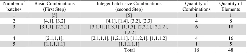
Table 1
The Integer Composition Method Results
Number of batches
Basic Combinations (First Step)
Integer batch-size Combinations (second Step)
Quantity of Combinations
Quantity of Elements
1 [5] [5] 1 1
2 [4,1], [3,2] [4,1], [1,4], [3,2], [2,3] 4 8
3 [3,1,1], [2,2,1] [3,1,1], [1,3,1], [1,1,3], [2,2,1], [2,1,2], [1,2,2]
6 18
4 [2,1,1,1], [2,1,1,1], [1,2,1,1], [1,1,2,1], [1,1,1,2] 4 16
5 [1,1,1,1,1] [1,1,1,1,1] 1 5
Total 16 48
Table 1 shows for 5 unit demands, there are 16 integer batch-size combinations and 48 elements. Shen and Evan (1996) have proved that n units demand will produce 2n-1 number of combinations and (n+1)2n -2 number of elements. Table 2 shows the examples of the total quantity of batch sizes combinations and
total quantity of elements for some number variety of demands.
Table 2
Testing Results for the number variety of demands
Demands (n) The total quantity of combinations (f(n)) The total quantity of elements
1 1 1
2 2 3
3 4 8
4 8 20
5 16 48
10 512 2,816
15 16,384 131.072
20 524,288 5.505.024
N 2n-1 (n+1)2n-2
Table 2 shows that both of the number of combinations and the number of elements increase in line with the increase of the number of demands. Based on Integer Composition method, It is proposed optimal algorithm (P-Algorithm) to solve the problems as follows.
[P-Algorithm]
Step 1: Input parameters n, d, p, s, δ, v, w, and tB. Continue to Step 2.
Step 2: Generate sets of all integer batch-size combinations by using the Integer Composition Algorithm. Continue to Step 3.
Step 3: For each of the alternative solution batch sizes:
Step 3.1: Calculate the processing time of batch (T[i]) using Eq. (8). Continue to Step 3.2
Step 3.2: Compute total actual flow time by using Eq. (9) with the constraints which are Eq. (10)-(14). Continue to Step 4.
Step 4: Find the solution that given minimum total actual flow time. STOP.
Numerical experiment for a model was conducted by giving the following input data parameters: n = 5,
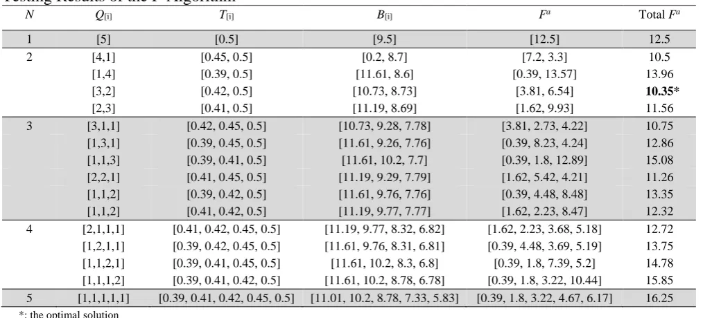
Table 3
Testing Results of the P-Algorithm
N Q[i] T[i] B[i] Fa Total Fa
1 [5] [0.5] [9.5] [12.5] 12.5
2 [4,1] [0.45, 0.5] [0.2, 8.7] [7.2, 3.3] 10.5
[1,4] [0.39, 0.5] [11.61, 8.6] [0.39, 13.57] 13.96
[3,2] [0.42, 0.5] [10.73, 8.73] [3.81, 6.54] 10.35*
[2,3] [0.41, 0.5] [11.19, 8.69] [1.62, 9.93] 11.56
3 [3,1,1] [0.42, 0.45, 0.5] [10.73, 9.28, 7.78] [3.81, 2.73, 4.22] 10.75 [1,3,1] [0.39, 0.45, 0.5] [11.61, 9.26, 7.76] [0.39, 8.23, 4.24] 12.86 [1,1,3] [0.39, 0.41, 0.5] [11.61, 10.2, 7.7] [0.39, 1.8, 12.89] 15.08 [2,2,1] [0.41, 0.45, 0.5] [11.19, 9.29, 7.79] [1.62, 5.42, 4.21] 11.26 [1,1,2] [0.39, 0.42, 0.5] [11.61, 9.76, 7.76] [0.39, 4.48, 8.48] 13.35 [1,1,2] [0.41, 0.42, 0.5] [11.19, 9.77, 7.77] [1.62, 2.23, 8.47] 12.32 4 [2,1,1,1] [0.41, 0.42, 0.45, 0.5] [11.19, 9.77, 8.32, 6.82] [1.62, 2.23, 3.68, 5.18] 12.72 [1,2,1,1] [0.39, 0.42, 0.45, 0.5] [11.61, 9.76, 8.31, 6.81] [0.39, 4.48, 3.69, 5.19] 13.75 [1,1,2,1] [0.39, 0.41, 0.45, 0.5] [11.61, 10.2, 8.3, 6.8] [0.39, 1.8, 7.39, 5.2] 14.78 [1,1,1,2] [0.39, 0.41, 0.42, 0.5] [11.61, 10.2, 8.78, 6.78] [0.39, 1.8, 3.22, 10.44] 15.85 5 [1,1,1,1,1] [0.39, 0.41, 0.42, 0.45, 0.5] [11.01, 10.2, 8.78, 7.33, 5.83] [0.39, 1.8, 3.22, 4.67, 6.17] 16.25 *: the optimal solution
The optimal number of batches (N) is 2, and batch sizes (Q[i]) are 3 and 2. Although the algorithm can
generate an optimal solution, it will take a long time to compute and also needs higher physical memory when the results are reported by computer. It is because the problems are solved in polynomial time complexity. The proof which is shown by Lemma and Proposition as follows.
Lemma1. All feasible integer batch-size combinations in Step 2 can be solved in running time n2n-1. Proof. Suppose there are n unit demands has 2n-1 integer batch-size combinations. It is proved by Shen
and Evan (1996) that the total number of combinations can be solved in running time T(n)=n2n-1. □
Lemma2. Batch processing time with simultaneous effect of learning and forgetting in Step 3.1 can be
solved in running time T(n)= (n+1)2n-2.
Proof. Shen and Evan (1996) prove there are (n+1)2n-2 elements of integer batch sizes. Batch processing
time with simultaneous effects of learning and forgetting can be solved in one-time complexity for each element. Thus, all element batch sizes can be solved in running time T(n)= (n+1)2n-2. □
Lemma3. The quantity of total actual flow time for all combinations in Step 3.2 can be solved in running time T(n)=2n-1.
Proof. Since the total number of integer batch-size combinations is equal with 2n-1, the total actual flow
time for all combinations can be solved in running time T(n)=2n-1. □
Lemma 4. The optimal solution of total actual flow time in Step 4 can be achieved in running time
T(n)=2n-1.
Proof. Since the quantity of total actual flow time for all combinations is equal with 2n-1, searching the
optimal solution of total actual flow time can be solved while running time T(n)=1. □
Proposition 1. The running time of batch scheduling problems for a single machine with the
simultaneous effects of learning and forgetting to minimize total actual flow time can be calculated using formula ( ) ( )
( )
1 ( )( )
21 2n 1 2n 1
T n = n+ − + n+ − + and it can be solved in a worst-case polynomial time
Proof. Based on Lemma 1, Lemma 2, Lemma 3, and Lemma 4, the running time of the problems can be formulated as follows.
( )
( )
1(
)
( ) ( )
2 12n 1 2n 2n 1
T n =n − + n+ − + − +
T(n) = O(g(n)) if and only if there is a positive real number c and a real number n0 such that:
( )
12n
T n ≤c n − where n≥n0.
Thus, the Big-O proved in the following condition as follows.
( ) ( )
( )
( )
( ) ( ) ( ) ( ) ( ) (
)
1 2 2 1 1 2 2 1
1 1 1 1 1 1
2 2 2 2 1 2 2 2 2 1
2 2 2 2 2 5 2
n n n n n n n n
n n n n n n
n n n n
n n n n n n
− − − − − − − −
− − − − − −
+ + + + ≤ + + + +
≤ + + + + ≤
If n0 =1 then there is exists a positive real number c, that is c=5 for all n≥n0 □
4.2 The Heuristic Solution
Since the problems proved by using Preposition 1, then it can be solved in a worst-case polynomial time complexity O(n2n-1), this research develops the heuristic solution based on the Lagrange Relaxation
method. The decision variables are the number of batches, batch sizes and the sequence of the resulting batches.
4.2.1. Determining Batch Sizes
The current research assumes that the batch sizes are integer. It is also considered that the processing time of parts in a batch scheduled at a position is different from that at the next position in backward scheduling approach. The learning and forgetting effect are started from the last position of batches to the first. It is proposed a backward computation for determining the batch sizes, that is, the calculation of the batch sizes are started from the last number of index to the first (i=N,..,1).
Halim et al. (1994) propose the formula for calculating the optimal batch sizes for single machine problems by using the Lagrange Relaxation as follows.
(
) (
)(
)( ) ( )
[i] / 1 / 2 1 / / , 1,...,
Q = n N + N+ s t − s t i i= N (15)
Eq. (15) can be re-written by using the backward computation as shown in the following equation.
(
)(
)( ) ( )
[i]
1
/ 1 / 2 1 / / , ,...,1
N
k k i
Q n Q i i s t s t i i N
= +
= − + + − =
∑
(16)
Substitute t in Eq. (16) by T[i] in Eq. (8) yields:
(
)(
)
(
[ ])
(
[ ])
[i]
1
/ 1 / 2 1 / / , ,...,1
N
k i i
k i
Q n Q i i s T s T i i N
= + = − + + − =
∑
(17) [ ](
[ ])
(
[ ] [ ])
[ ] 1where min max 1 1 i 1 , ,
m f
N N
i k i k k i k i
T p Q X Y v w
− + = = = + + + −
∑
∑
Applying Constraint (13) and Eq. (17) simultaneously yields:
( )(
)
(
[ ])
(
[ ])
[i]
1
max / 1 / 2 1 / / , 1 , ,...,1
N
k i i
k i
Q n Q i i s T s T i i N
4.2.2 Determining the Maximum Number of Batches
The optimal number of batches cannot be determined precisely because batch processing time depend on its position on a schedule. The maximum number of batches can be calculated by assuming that all parts in all batches are processed on a machine by the minimum value of batch processing time. According to Constraints (11) and (14), the maximum number of batches (Nmax) can be calculated as follows.
(
)
{
min}
max min / 1,
N = d−nT s+ n (19)
T minimum can be relaxed using the formula:
(
)
{
}
min max 1 m,
T ≈ p +n − v (20)
Eq. (20) shows that minimum batch processing time is found when all parts are proceeded together and no forgetting effect. Substitute Tmin in Eq. (19) by Eq. (20) yields:
(
)
{
}
(
)
(
)
{
}
max min max 1 m, 1 ,
N = d−n p +n − v s+ n
(21)
Based on Eq. (14) and Eq. (21), it also can be observed that the optimal value of total actual flow time is within the closed interval [1, Nmax]. Lemma says as follows.
Lemma 5. If the objective function of total actual flow time is convex in a closed interval [1, Nmax], then the optimal value of total actual flow time is within the interval.
Proof. The optimal number of batches should be convex in a closed interval [1, Nmax] if and only if
Hessian Matrix is a definite positive. f: Rn→Rconvex function ↔ H
f (x) is a definite positive.
Based on Eq. (8), T[i] is the function of Q, s, tB, f, and δ. It is defined dependent variable T[i] as a parameter,
i.e T[i] as t. Eq. (10) can be re-written as follows.
( )
[ ]( )
[ ]( )
[ ] [ ]2 2
1 1 1 1
1 / 2 1 / 2
N N N N
a
i i i i
i i i i
f x F s iQ t Q t Q s Q
= = = =
= = + + −
∑
∑
∑
∑
Gradient: [ ] [ ]
1
/
N
i i
i
F Q si tQ t Q s
=
∂ ∂ = + + −
∑
[ ]
( )
[ ] [ ]2
/ N 1 / 2 N N
F N sNQ tQ sQ
∂ ∂ = + −
Hessian Matrix:
( )
( )
[ ]
2 0
0
f
N t
H x f x
sQ
= ∇ =
Using Silvester Criterion yields:
[ ] [ ]
0
det 0
0 N
N t
tsQ
sQ → >
Hessian Matrix is a definite positive. Therefore, the objective function is convex. The optimal number of batches is within the interval of [1, Nmax]. □
4.2.3 Determining Sequence of the Resulting Batches
Proposition 2. Minimizing total actual flow time in batch scheduling problems on single-machine with
Proof. There are two feasible schedules for N batches. The first schedule places batch of (i)-th position at the (i)-th position and batch of (i+1)-th position to the (i+1)-th position. The last schedule is only different from the first schedule in batch of (i)-th position at the (i+1)-th position and batch of (i+1)-th position at the (i)-th position. Both of them are arranged by using backward scheduling approach. If Fa1 and Fa2 are the value of total actual flow time for the first schedule and the second respectively, the following is obtained
(
[ ])
(
[ ])
1 2
[ ] [ 1] [ 1] 1 [ 1] [ ] [ ]
a a
i i i i i i
i i
F −F = T Q Q + +sQ + − T+ Q + Q +sQ
The value of total actual flow time at the first schedule will be less than or equal to that value at the second schedule if only if
(
T Q[ ]i [ ]i +s Q)
[i+1] ≤(
T[ ]i+1Q[i+1]+s Q)
[ ]i or T[ ]i +s Q/ [ ]i ≤T[ ]i+1 +s Q/ [i+1]The value of total actual flow time at the left side will be less than the right side if the batch size at the left side is greater than the right side. Therefore, minimizing total actual flow time can be obtained by arranging the batches in order to the LPT rule in the backward scheduling approach.
(
T Q[ ]1 [1]+s)
/Q[1]≤(
T Q[ ]2 [2]+s)
/Q[2]≤ ≤...(
T Q[ ]N [N]+s)
/Q[N].□Based on the Lagrange Relaxation method, it is proposed heuristic algorithm (H-Algorithm) to solve the problems as follows.
[H-Algorithm]
Step 1: Input parameters n, d, p, s, δ, v, w, and tB. Continue to Step 2.
Step 2: Find Nmaxby Eq. (21). Determine j as an index for the number of batches (j= 1, …, Nmax). Continue to Step 3.
Step 3: Begin with j = 1. Determine Q[1] = n, T[1] = p. Continue to Step 4.
Step 4: Calculate the value of M = np. If M≤ d, then continue to Step 5, otherwise STOP because the demand cannot be scheduled.
Step 5: Calculate total actual flow time for j =1by Eq. (9). Determine the value of F[1] as F*. Continue
to Step 6.
Step 6: Determine the index of the number of batches j=j+1. If j <Nmax, continue to Step 7, otherwise determine F* as the best solution and then STOP.
Step 7: Determine N=j. Set Q[N+1]=0, T[N+1]=0. Continue to Step 8.
Step 8: Calculate the processing time of batch (T[i]) using Eq. (8) and the batch sizes (Q[i]) using Eq.
(18). Continue to Step 9.
Step 9: Based on Proposition 2, sequence the resulting batches in a non-increasing size of Q[i] in
backward scheduling approach. Continue to Step 10.
Step 10: Calculate M =
∑
iN=1T Q[ ] [ ]i i +(
N−1)
s. If M≤ d, continue to Step 11, otherwise determine F* as the best solution and then STOP.Step 11: Compute total actual flow time for j by Eq. (9). Continue to Step 12.
Step 12: Compare the value of total actual flow time F[j] and F*. If F[j] < F*, determine F[j] as F* and
then return to Step 6, otherwise determine F* as the best solution and then STOP.
Numerical experimenttest was conducted by giving the following input data parameters: n = 5, d = 12,
Table 4
Testing Results of the H-Algorithm
N i Q[i] T[i] B[i] Total Fa
1 1 5 0.5 9.5 12.5
2 1 3 0.42 10.73 10.35*
2 2 0.5 8.73
3 1 3 0.42 10.73 10.75
2 1 0.45 9.28
3 1 0.5 7.78
*: the best solution
Thus, the total actual flow time for N=2 is temporarily best solution. The search of the solution continues for N=3. The result of the total actual flow time is 10.75. The total actual flow time for N=3 is compared with N=2, and it is found that the total actual flow time for N=2 is smaller than N=3. Thus, the algorithm is stopped by determining that the total actual flow time is 10.35 as the best solution obtained at N=2. For this case, the best solution of the H-Algorithm is equal to the optimal solution of the P-Algorithm.
4.3 Comparison test
The tests are continued by testing the optimality of both proposed algorithms. They are carried out by comparing the solution of the P-Algorithm and the H-Algorithm. The P-Algorithm and the H-Algorithm are coded in C++, and the results are reported by using computer processor Intel Core i3 with 6 GB of Random Access Memory (2 GB usable in 64-bit of platform) and 1 GB of Graphical Processor Unit. The comparison tests have been done on more than 100 problems. The results of comparison test show that the H-algorithm works adequately for any numbers of demands. However, it does not guarantee to produce an optimal solution. Meanwhile, the P-Algorithm guarantee to produce the optimal solution but it is only adequate for demands less than 23 units (small size problems). If there are more than 23 unit demands, the solution can not be found because of out-of-memory (o.o.m). In order to make well understanding of the behavior of comparison tests, Table 5 shows the examples of comparison tests for 10 problems where input parameters are generated randomly.
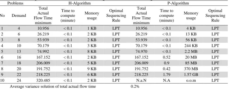
Table 5
The result of comparison test between the H-Algorithm and the P-Algorithm
Problems H-Algorithm P-Algorithm
No Demand
Total Actual Flow Time
minimum
Time to compute (minute)
Memory usage
Optimal Sequencing
Rule
Total Actual Flow Time
minimum
Time to compute (minute)
Memory usage
Optimal Sequencing
Rule
1 4 10.956 < 0.1 1 KB LPT 10.956 < 0.1 4 KB LPT
2 6 26.219 < 0.1 2 KB LPT 26.219 < 0.1 13 KB LPT 3 8 53.939 < 0.1 2 KB LPT 53.939 < 0.1 56 KB LPT 4 10 70.179 < 0.1 3 KB LPT 70.179 < 0.1 244 KB LPT 5 13 74.992 < 0.1 8 KB LPT 74.970 < 0.1 2.2 MB LPT
6 16 167.152 < 0.1 2 KB LPT 167.152 0.52 20 MB LPT
7 18 206.009 < 0.1 5 KB LPT 206.009 0.9 85 MB LPT
8 20 191.752 < 0.1 9 KB LPT 191.752 0.42 370 MB LPT 9 22 218.225 < 0.1 6 KB LPT 218.225 1.79 1.57 GB LPT
10 24 320.485 < 0.1 2 KB LPT N.a.N N.A o.o.m LPT
Average variance solution of total actual flow time 0.2%
approach. It also shows that the H-Algorithm takes time to compute, and uses memory less than the P-Algorithm.
5. Concluding Remarks
The current research deals with single-machine batch scheduling problems with the simultaneous effect of learning and forgetting to minimize total actual flow time. The problems are proved by using the Integer Composition method can be solved in a worst-case polynomial time complexity O(n2n-1). This paper proposes two algorithms to solve these problems. The first algorithm produces the optimal solution that is developed by using the Integer Composition method. The second algorithm is the heuristic algorithm that is developed based on the Lagrange Relaxation method. Although the heuristic algorithm does not guarantee to produce an optimal solution, numerical experiments on randomly generated examples show that the heuristic algorithm gives outstanding results. The model introduced in this paper can be extended to discuss batch scheduling problems with learning and forgetting effects, as well as deterioration simultaneously. In a real system, it is also known that the changes in processing times occur not only on the operators but also on the machines.
Acknowledgments
The authors wish to thank the editors and the referees for their constructive comments and suggestions.
References
Anzanello, M.J. & Foglianto, F. S. (2010). Scheduling learning dependent jobs in customized assembly lines. International Journal of Production Research, 48, 6683-6699.
Arzi, Y. & Shtub, A. (1997). Learning and forgetting in mental and mechanical tasks: A comparative study. IIE Transactions, 29 759-768.
Baker, K.R. & Trietsch, D. (2009). Principles of sequencing and scheduling. John and Wiley & Sons. Biskup, D. (1999). Single machine scheduling with learning considerations. European Journal of
Operational Research, 115, 173-178.
Carlson, J. G. & Rowe, A. J. (1976). How much does forgetting cost?, Industrial Engineering, 8 40-47. Chen, C.K., Lo, C.C. & Liao, Y.X. (2008). Optimal lot size with learning consideration on an imperfect
production system with allowable shortages. International Journal of Production Economics, 113, 459-469.
Cheng, T.C.E, Lee, W.C. & Wu, C. C. (2010). Scheduling problems with deteriorating jobs and learning effects including proportional setup times. Computers & Industrial Engineering, 58, 326–331.
Cheng, T.C.E. (1991). An EOQ model with learning effect on set-ups. Production and Inventory
Management, 32, 83-84.
Cheng, T.C.E. (1994). An economic manufacturing quantity model with learning effect. International
Journal of Production Economics, 33, 257-264.
Cheng, T.C.E., Kuo, W.H. & Yang, D.L. (2013). Scheduling with a position-weighted learning effect based on sum-of-logarithm-processing-times and job position. Information Sciences, 221, 490–500. Cheng, T.C.E., Lai, P.J., Wu, C.C. & Lee, W.C. (2009). Single-machine scheduling with
sum-of-logarithm-processing-times-based learning considerations. Information Sciences, 179, 3127–3135. Cheng, T.C.E., Wu, W.H., Cheng, S.R. & Wu, C.C. (2011). Two-agent scheduling with position-based
deteriorating jobs and learning effects. Applied Mathematics and Computation, 217, 8804–8824. Chiu, H.N. & Chen, H.M. (2005). An optimal algorithm for solving the dynamic lot-sizing model with
learning and forgetting in set-ups and production. International Journal of Production Economics, 95, 179-193.
Chiu, H.N. (1997). Discrete-time varying demand lot-size models with learning and forgetting effect.
Production Planning Control, 8, 484-493.
Dobson, G., Karmakar, U. S. & Rummel, J. (1987). Batching to minimize flow times on one machine.
Management Science, 33, 784-799.
Gaweijnowics, S. (1996). A note on scheduling on a single processor with speed dependent on a number of executed jobs. Information Processing Letters, 57, 297-300.
Halim, A.H. & Ohta, H. (1994). Batch Scheduling Problems to minimize inventory cost in the shop with both receiving and delivery Just-In-Time. International Journal of Production Economics, 33, 185-194.
Halim, A.H., Miyazaki, S. & Ohta, H. (1994). Batch scheduling problems to minimize actual flow times of component through the shop under JIT environment. European Journal of Operational Research, 72, 529-544.
Jaber, M.Y. (2011). Learning Curves: Theory, model, and applications, Taylor & Francis Group, US. Jaber, M.Y. & Bonney, M. (1996). Production break and the learning curve: The forgetting phenomenon.
Applied Mathematical Modelling, 20, 162-169.
Jaber, M.Y. & Salamah, M.K. (1995). Optimal lot sizing under learning considerations: Shortages allowed and back ordered. AppliedMathematicalModeling, 19, 307-310.
Janiak, A., Lichtensteind, M. & Rusoń, A. (2011). Scheduling jobs with a linear model of simultaneous ageing and learning effects. Decision Making in Manufacturing and Services, 5, 37–48.
Ji. M. & Cheng, T.C.E. (2010). Batch scheduling of simple linear deteriorating jobs on a single machine to minimize makespan. European Journal of Operational Research, 202, 90-98.
Keachie, E.C. & Fontana, R.J. (1966). Effect of learning on optimal lot size. Management Science, 13, B102-B108.
Kuo, W.H. & Yang, D.L. (2006), Minimizing the total completion time in a single-machine scheduling problem with a time-dependent learning effect. European Journal of Operational Research, 174, 1184-1190.
Lai, P.J. & Lee, W.C. (2013). Single machine scheduling with learning and forgetting effect. Applied
Mathematical Modelling, 37, 4509-4516.
Li, C.L. & Cheng, T.C.E. (1994). An economic production quantity model with learning and forgetting considerations. Production and Operations Management, 3, 118-132.
Morton, T.E. & Pentico, D.W. (1993). Heuristic scheduling systems. John Wiley & Sons, Inc.
Nembhard, D.A. & Uzumeri, M.V. (2000). Experiential learning and forgetting for manual and cognitive tasks. International Journal of Industrial Ergonomics, 25, 315–326.
Pinedo, M. (2002). Scheduling: Theory, algorithms, and systems. Prentice Hall, New Jersey.
Shen, H. & Evans. D. J. (1996). A new method for generating integer compositions in parallel. Parallel
Algorithms Applications, 9, 101-109.
Steedman, I. (1970). Some improvement curve theory. International Journal Production Research, 8, 189-206.
Teyarachakul, S., Chand, S. & Ward, J. (2008). Batch sizing under learning and forgetting: Steady state characteristics for the constant demand case. Operations Research Letters, 36, 589-593.
Teyarachakul, S., Chand, S. & Ward, J. (2011). Effect of learning and forgetting on batch sizes.
Production and Operations Management, 20, 116-128.
Wang, X. & Cheng, T.C.E., (2007). Single machine scheduling with deteriorating jobs and learning effects to minimize the makespan. European Journal of Operational Research, 178, 57 -70.
Wright, T.P. (1936). Factors affecting the cost of airplanes. Journal of Aeronautical Sciences, 3, 122-128.
Wu, C.H., Lai, P. J. & Lee, W. C. (2014). A note on a single machine scheduling with sum of processing time based on learning and forgetting effects. Applied Mathematical Modelling, 39, 415-424.
Yang, W.H. & Chand, S. (2008). Learning and forgetting effect on a group scheduling problem.