An Analog VLSI Motion Sensor
Based on the Fly Visual System
Thesis by
Reid
R.
Harrison
In Partial Fulfillment of the Requirements for the Degree of
Doctor of Philosophy
c-o o
't-California Institute of Technology Pasadena, California
2000
Acknowledgements
I would first like to thank my parents, Don and Lesa Harrison, for instilling a love of science in me at a very young age, for nurturing my intellectual interests for as long as I can remember, and for providing unconditional love and support as I explored and grew.
lowe many thanks to my advisor and Doktorvater Prof. Christof Koch, who gave me both freedom and support to pursue my vision. His guidance and encouragement made this work possible.
I thank my thesis committee: Prof. Michael Dickinson, Prof. Rodney Goodman, Prof. Gilles Lau-rent, and Prof. Pietro Perona for reading my dissertation and providing a supportive environment. I also thank Prof. Jim Bower and Prof. Mark Konishi for serving on my Ph.D. candidacy committees. I thank the Defense Advanced Research Projects Agency (DARPA), the Office of Naval Research (ONR), the National Institute of Mental Health (NIMH), and the National Science Foundation's Engineering Research Center (ERC) for Neuromorphic Systems Engineering at Caltech, for funding my research over the years.
Many people have enriched my academic experience during the past five years, and some have become good friends. Among those contributing to my growth as a scientist and engineer are: Axel Borst, Tobi Delbruck, Rainer Deutschmann, Chris Diorio, Rodney Douglas, Martin Egelhaaf, Volker Gauck, Jurgen "Bulle" Haag, Paul Hasler, Chuck Higgins, Tim Horiuchi, Giacomo Indiveri, Vincent Koosh, Jorg Kramer, Oliver Landolt, Shih-Chii Liu, Ania Mitros, Brad Minch, Alberto Pesavento, Rahul Sarpeshkar, Theron Stanford, and Barbara Webb. I thank you for sharing your knowledge and enthusiasm with me. Thanks are also due to Candi Maechtlen and Margaret Lindstrom for administrative assistance and advice.
I would also like to thank many friends at Caltech who have kept me sane and given me fond memories of my time in Pasadena: Stephen Glade, Adrian Hightower, Peter Bogdanoff, Andy Wa-niuk, Anthony Leonardo, Michael Gibson, Fidel Santamaria-Perez, Zsuzsi Hamburger, Alyssa Apsel, Angie Louie, Eric Slimko, Grace Chang, Sarah Laxton, Jennie Yoder, and Mika Nystrom.
Abstract
Contents
Acknowledgements
Abstract
1 Introduction
2 Sensory Systems of the Fly 2.1 The Visual System of the Fly
2.1.1 Photoreception . . . . 2.1.2
2.1.3 2.1.4
Signal Processing in the Peripheral Optic Lobe The Tangential Cells of the Lobular Plate Visually Guided Behaviors
2.2 The Vestibular Sense 2.3 Other Sensors
2.3.1 Ocelli
2.3.2 Polarized Light. Detection 2.3.3 Linear Acceleration. . . .
3 Motion Detection - Algorithms and VLSI Implementation 3.1 Feature-Based Motion Detection . . . . .. . . .
3.1.1 Motion Detectors Using Spatial Feature Detect.ors 3.1.2 Motion Detectors Using Temporal Feature Detectors 3.1.3 The Obliquity Problem
3.1.4 The Aperture Problem. 3.1.5 Noise . . . . 3.2 Intensity-Based Motion Detection.
3.2.1 The Gradient Model . . . . 3.2.2 Correlation-Based Motion Detection 3.3 Hassenstein-Reichardt Model in Detail
3.3.1 Theoretical Analysis . .. . 3.3.2 Hardware Implementations
4 VLSI Reichardt Detector Design
4.1 Current-Mode Design
4.2 Voltage-Mode Design.
4.2.1 Circuit Architecture
4.2.2 Supply Voltage Requirements 4.2.3 Matching Considerations
5 VLSI Motion Detector Characterization 5.1 Methodology . . . .
5.2 Direction Selectivity 5.3 Response to Simple Stimuli
5.3.1 Motion Onset 5.3.2 Motion Offset 5.3.3 Directional Tuning
5.4 Spatiotemporal Frequency Tuning
5.5 Contrast Dependence . 5.6 Interpixel Variation ..
5.7 Response to Naturalistic Stimuli
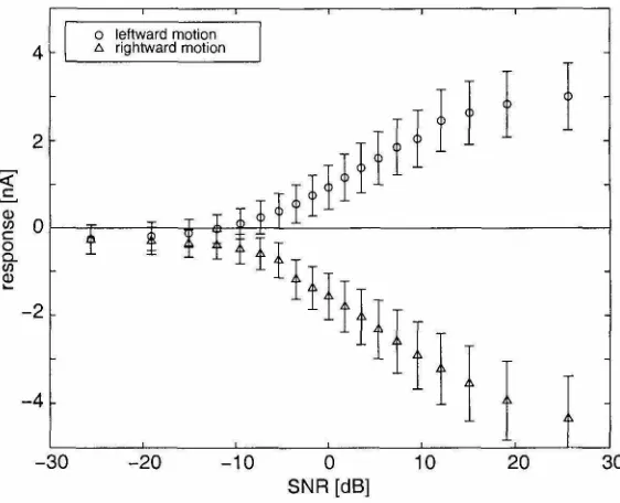
5.8 Robustness to Noisy Stimuli .
5.9 Speed Tuning .. .
5.10 Power Dissipation
6 Stimulus Reconstruction
6.1 Stimulus Reconstruction Techniques . . . . . 6.2 Pattern Velocity Estimation by Fly Interneurons 6.3 Pattern Velocity Estimation by Silicon EMD Array .
7 Optomotor Control
7.1 Measuring the Optomotor Response . . . .. .
7.1.1 Experiments Previously Performed on Flies
7.1.2 Duplicating Experiments with the Silicon System
7.2 Application to Autonomous Vehicle Control
7.3 Robot Optomotor System . . . . 7.3.1 Hardware Implement.ation
7.3.2 Robot Experiments .. . .
8 Nonlinear Spatial Integration
8.1 Gain Control in Fly Tangential Neurons 8.2 Algorithm and Biological Architecture
8.3 Silicon Implementation.
8.4 Experiments . . . .
8.4.1 Varying Pattern Size
8.4.2 8.4.3
Varying Leakage Conductance
Power Dissipation
9 System Integration
9.1 Visual Motion Sensors and Their Limitations
9.2 Coriolis-Force Gyroscopes and Their Limitations
10 Conclusions
Bibliography
81
81
82
84
85
85 85 86
91
91
93
95
List of Figures
2.1 Central Nervous System of the Fly . . . . 2.2 Number of Pixels in Biological and Silicon Systems 2.3 The Halteres of the Blowfly Ca.lliphom.
3.1 The Correspondence Problem 3.2 The Obliquity Problem
3.3 Reichardt Motion Detector Architecture
4.1 Current-Mode EMD Sub circuits 4.2 Voltage-Mode EMD Subcircuits . 4.3 Voltage-Mode Motion Detector Layout 4.4 Layout of EMD Circuits on a Chip
5.1 Chip Testing Methodology. 5.2 Direction Selectivity . . . .
5.3 Motion Onset and Offset in the HS Neuron 5.4 Motion Onset: Leftward Motion
5.5 Motion Onset: Rightward Motion. 5.6 Motion Offset: Leftward Motion 5.7 Motion Offset: Rightward Motion.
5.8 Directional Tuning of Reichardt Detector Array. 5.9 Directional Tuning of Fly Lobular Plate Neurons 5.10 Temporal Frequency Sensitivity
5.ll Spatial Frequency Sensitivity .
5.12 Temporal Frequency Tuning in Fly Neurons 5.13 Spatiotemporal Frequency Tuning . . . 5.14 Spatiotemporal Frequency Tuning in Fly Neurons. 5.15 Tuning the Temporal Frequency Response
5.16 Contrast Sensitivity 5.17 Interpixel Variation .
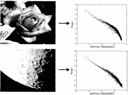
5.18 1/
f
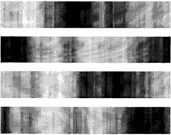
Spatial Frequency Spectra in Natural Scenes. 5.19 Example of Random "Natural" Patterns5.20 Chip Response to 1/
f
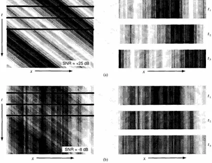
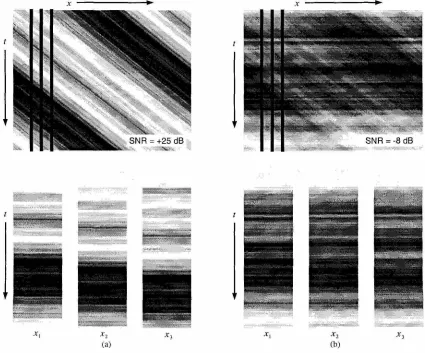
Patterns . . .5.21 Adding Spatial Noise .. 5.22 Adding Temporal Noise
5.23 Robustness with Spatial Noise. 5.24 Robustness with Temporal Noise 5.25 Speed Tuning . . . . . .
6.1 Stimulus Reconstruction in the HS Neuron. 6.2 Coherence Functions for Fly HS Cell. . . . 6.3 Signal and Noise Spectra for Fly HS Cell.
6.4 Stimulus Reconstruction in the Silicon EMD Array .. 6.5 Coherence Functions for Silicon EMD Array.
6.6 Signal and Noise Spectra for Silicon EMD Array. 6.7 Coherence Function for Fly and Silicon EMDs.
7.1 Experimental Methodology 7.2 Fly's Optomotor Behavior .
7.3 The Optomotor Behavior of our Silicon System 7.4 Schematic of Optomotor System . . .
7.5 Photograph of the Optomotor System 7.6 Asymmetrical Gear Ratios . . . . 7.7 Visual Environment During Experiments. 7.8 Robot Path with No Sensory Feedback. 7.9 Robot Path with Sensory Feedback. 7.10 Histogram of Angular Velocities.
8.1 8.2 8.3 8.4 8.5 8.6 8.7 9.1 9.2
Gaps in Optic Flow Fields . . . .
Gain Control in a Wide-Field Motion-Sensitive Neuron in the Fly. Models of Wide-Field Motion-Sensitive Neurons in the Fly. Weak Direction Selectivity. . .
Variable Conductance Circuits Gain Control in the Silicon System Varying Leakage Conductance.
Antibump Circuit. . . . Antibump Circuit Data
Chapter
1
Introd uction
Engineers have long looked to nature for inspiration. The diversity of life produced by five billion years of evolution provides countless existence proofs of organic machines with abilities that far surpass those of our own relatively crude automata. We have learned how to harness large amounts of energy and thus far exceed the capabilities of biological systems in some ways (e.g., supersonic flight, space travel, and global communications). However, biological information processing systems (i.e., brains) far outperform today's most advanced computers at tasks involving real-time pattern recognition and perception in complex, uncontrolled environments. If we take energy efficiency into account, the performance gap widens. The human brain dissipates 12 W of power, independent of mental activity. A modern microprocessor dissipates around 50 W, and is equivalent to a vanishingly small fraction of our brain's functionality.
Indeed, the human brain is a daunting goal for biologists and engineers alike. Our brain takes several years to fully develop, and contains between 1010 and 1011 neurons (nerve cells), each com-municating with 103 other cells, on average. Brains of other animals (particularly invertebrates) are much smaller but still perform remarkably complex computations. Insect brains, for example, typically contain between 105 and 106 neurons. As we shall see in the following chapter, insects perform sophisticated information-processing tasks rapidly and efficiently.
In this body of work, we have attempted to extract computational principles from the visual system of the fly and apply these principles to an engineered system-an integrated, low-power visual motion sensor. As our engineering tool we use very-large scale integration (VLSI) of silicon circuits-the most advanced information-processing substrate available today. In particular, we explore continuous-time (unclocked), continuous-value (analog) circuit architectures. This approach was pioneered by Mead and colleagues beginning the in 1980s (Mead, 1989).
Chapter 2
Sensory Systems of the Fly
The fly is an attractive target for biologically-inspired approaches to engineering. Its brain and sensory systems have been studied for decades, so much is known about their operation. Of course, we are still decades (or centuries) away from understanding the entire system, but a wealth of behavioral and electrophysiological data has led to the development of several models of information processing.
Flies possess a diverse array of organs for sensing their environment. In addition to the fa-miliar sense of vision, flies employ Coriolis-force "gyroscopes," polarized light sensors, and body proprioception to aid in navigation. In this chapter, we will discuss these sensory systems.
2.1
The Visual System of the Fly
Vision is a vitally important sense for flying insects. In the housefly's brain, over half of the 350,000 neurons are believed to have some role in visual processing. The fly's optic lobes contain motion-sensitive neurons which respond to moving stimuli over large portions of the visual field. Many of these neurons have been linked to specific visually-guided behaviors that help the animal navigate through a complex environment in a robust manner (Egelhaaf and Borst, 1993).
Insects process visual motion information in a local, hierarchical manner. This information processing begins at the sensor-the retina (see Figure 2.1). Despite the multi-lens construction of the compound eye, the pattern projected onto the underlying retina is a single image of the visual scene. Photoreceptors in the retina adapt to the ambient light level, and signal temporal deviations from this level. These signals are passed on to the next layer of cells, the lamina. Lamina cells generally show transient or highpass responses, emphasizing temporal change (Weckstrom et al., 1992). The next stage of processing is the medulla, a layer of cells that are extremely difficult to study directly due to their small size. Indirect evidence suggests that local measures of motion (i.e., between adjacent photoreceptors) are computed here. These local, direction-selective motion estimates are integrated by large tangential cells in the lobular plate (Hausen and Egelhaaf, 1989). The housefly has 50-60 tangential cells in each hemisphere of its brain. These are the best-studied cells in the fly visual system, and much is known about their properties.
retina
flJll""""'-lamma
250 J.1m
Figure 2.1: Central nervous system of the fly. Lenses in each compound eye focus light onto the retina. Photoreceptor signals are transmitted to the lamina, which emphasizes temporal change. A retinotopic arrangement is maintained through the medulla. The lobular plate contains wide-field, motion-sensitive tangential neurons that send information to the contralateral optic lobe as well as to the thoracic ganglia, which control the wings and legs. Adapted from Borst and Haag, 1996.
only to small objects moving across the visual field (Egelhaaf, 1985). It is believed that these "figure detection" cells allow the fly to locate nearby objects through motion parallax (Kimmerle et al., 1997). All of these sensory abilities require that motion first be detected locally between every pair of photoreceptors.
2.1.1
Photoreception
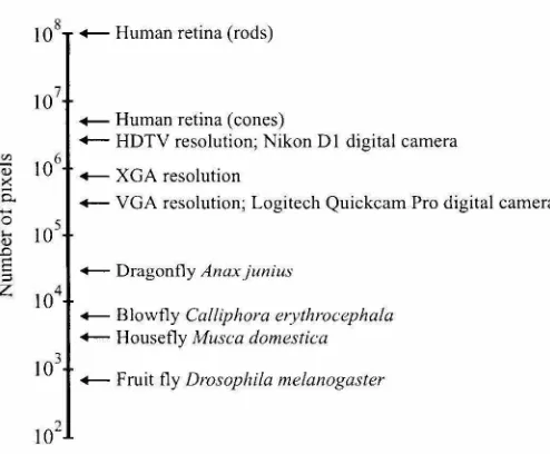
Each eye of the blowfly Calliphora erythrocephala consists of approximately 6000 individual lenses. Beneath each lens is a cluster of eight light-sensitive cells. Each lens and its associated photore-ceptors forms a unit called an ommatidium. Six of the eight photorephotore-ceptors are used to implement neural superposition, a technique to increase the effective lens diameter by pooling the responses of neighboring ommatidia. The other two photoreceptors do not seem to be involved in the detection of motion. Mutants with these photoreceptors impaired cannot discriminate colors, but show no motion-related deficits (Heisenberg and Buchner, 1977). From an information-processing perspec-tive, each ommatidium records one "pixel" of the external world's image. Interommatidial angular spacing is 1.1-1.3° (Land, 1997). This angular resolution is approximately 150 times worse than the 0.008° resolution in foveated region of the human retina (Wandell, 1995). (This is roughly equivalent to having 20/3000 vision.)
108 +-Human retina (rods)
+-Human retina (cones)
+-HDTV resolution; Nikon Dl digital camera 10
6
+-XGA resolution
+-VGA resolution; Logitech Quickcam Pro digital camera
+-Dragonfly Anaxjunius 104
+-Blowfly Calliphora erythrocephala +-Housefly Musca domestica 103
+-Fruit fly Drosophila melanogaster
Figure 2.2: Number of pixels in biological and silicon systems. Current state-of-the-art silicon imagers have numbers of pixels approaching human retina levels. Flying insects get by with orders of magnitude fewer pixels. All data is for single eyes. Human retina data from Wandell, 1995; insect data from Land, 1997.
contains only 700 ommatidia, resulting in an equivalent array size of 26 x 26 (Land, 1997). Today's cheap digital cameras provide 640 x 480 pixel images, and emerging photo-quality digital cameras provide 1800 x 1200 pixels or more~around two orders of magnitude more photoreceptors than a fly's eye (see Figure 2.2). Typical cameras concentrate these pixels into a 40° field of view, while each fly eye sees nearly a complete hemisphere.
It is remarkable that flies are capable of such impressive navigation when one considers their low-resolution eyes. This limited spatial acuity is a consequence of the compound eye design. In order to increase spatial acuity, more ommatidia are required. However, the resolving capability of each ommatidium is limited by diffraction, so each lens must also be made larger. If we wanted to build a compound eye with the acuity of the human fovea (0.008°), it would have a radius of 11.7 meters! The visual acuity of the largest insect eye in nature (that of the aeschnid dragonfly) reaches 0.24° in its most acute zone, still 30 times coarser than the human fovea (Land, 1997).
While inferior to human eyes spatially, fly vision far exceeds ours temporally. Human vision is sensitive to temporal modulations up to 20 or 30 Hz, while fly photoreceptors respond to temporal frequencies as high as 300 Hz (Autrum, 1958).
2.1.2
Signal Processing in the Peripheral Optic Lobe
[image:13.540.158.405.69.273.2]5
level but amplify temporal changes (Weckstrom et al., 1992). This highpass response has been shown to optimize information transfer through this region (Laughlin, 1994). Laminar cells do not exhibit motion-specific responses. There is a strong retinotopic organization from the retina through the lamina to the next layer, the medulla. Every ommatidia has an associated neural "cartridge" beneath it in these underlying ganglia, suggesting many identical processing units operating in parallel (Strausfeld, 1976).
Cells in this second optic ganglion are extremely small and difficult to record from, and little is know about their structure or function. DeVoe recorded from medullar cells in Calliphora and re-ported a wide variety of response characteristics: transient temporal responses, sustained responses, directional motion responses, and nondirectional motion responses (DeVoe and Ockleford, 1976; DeVoe, 1980).
2.1.3
The Tangential Cells of the Lobular Plate
The third optic ganglion is also known as the lobula-Iobular plate complex. At this point in the optic lobe, the retinotopic organization ends with massive spatial convergence. Information from several thousand photoreceptors converges onto 50-60 tangential cells. These cells have broad dendritic trees that receive synaptic input from large regions of the medulla, resulting in large visual receptive fields (Hausen, 1982a; Hausen, 1982b; Hengstenberg, 1982; Hausen, 1984; Krapp and Hengstenberg, 1996).
A subset of these neurons were found to respond primarily to horizontal motion, and these cells were given names beginning with 'H'. HI is a spiking neuron that responds to back-to-front optic flow. HSS, HSE, and HSN are graded potential (nonspiking) neurons covering the southern, equatorial, and northern regions of the visual field, respectively. Collectively called the HS cells, these neurons are depolarized by full-field visual motion from the front to the back of the eye, and hyperpolarized by back-to-front motion. They have been shown to encode horizontal motion as effectively as the spiking HI cell (Haag and Borst, 1997). Each HS cell integrates signals from an ipsilateral retinotopic array of elementary motion detectors (EMDs), units in the medulla that estimate local motion in small areas of the visual field. The HS cells synapse onto descending, spiking neurons which relay information to the motor centers of the thoracic ganglion. Another class of neurons, the VS cells, respond to vertical motion. Recently, it has been shown that these HS and VS cells are not simply responsive to motion along one axis, but rather act as matched filters for complex patterns of optic flow that would be produced by body rotations (Krapp and Hengstenberg, 1996).
2.1.4
Visually Guided Behaviors
Flies rely heavily on visual motion information to survive. In the fly, motion information is known
to underlie many important behaviors including stabilization during flight, orienting towards small,
rapidly-moving objects (Egelhaaf and Borst, 1993), and estimating time-to-contact for safe landings
(Borst and Bahde, 1988). Some motion-related tasks like extending the legs for landing can be
executed less than 70 ms after stimulus presentation. Wagner reports a 30 ms reaction time for
male flies chasing prospective mates (Wagner, 1986). The computational machinery performing this
sensory processing is fast, small, low-power, and robust.
Flies use visual motion information to estimate self-rotation and generate a compensatory torque
response to maintain stability during flight. This well-studied behavior is known as the optomotor
response. It is interesting from an engineering standpoint because it extracts relevant information
from a dynamic, unstructured environment on the basis of passive sensors and uses this information
to generate appropriate motor commands during flight. This system is implemented in biological
hardware that is many orders of magnitude smaller and more power efficient than CCD imagers
coupled to a conventional digital microprocessor.
Much of the computation underlying the optomotor control system is performed by the HS cells
(Geiger and Niissel, 1981; Geiger and Nassel, 1982; Egelhaaf et al., 1988; Hausen and Wehrhahn,
1990; Egelhaaf and Borst, 1993). This well-studied system estimates rotation from optic flow and
uses this information to produce a stabilizing torque with the wings (GCitz, 1975; Warzecha and
Egelhaaf, 1996).
Flies also use visual motion information to coordinate landings. Behavioral and modeling studies
indicate that such "time-to-Ianding" estimation could be produced by a temporal integration of
HS-type neurons sensitive to expanding optic flow patterns (Borst and Bahde, 1988; Borst, 1990). A
similar visual capability allows flies to avoid rapidly approaching predators. This escape response is
sensitive to motion as well as to decreases in light intensity (Holmqvist and Srinivasan, 1991).
Behavioral experiments both with freely-flying and tethered flies demonstrate the ability to
discriminate objects from background using relative motion (parallax) cues (Kimmerle et al., 1996;
Kimmerle et al., 1996). The FD cells mentioned above are thought to underlie this capability.
2.2
The Vestibular Sense
Dipterans (true flies and mosquitos) possess a remarkable evolutionary specialization for measuring
angular velocity. The hind wings of these animals evolved from flight surfaces into dedicated angular
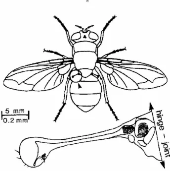
rate "gyroscopes." These halteres, as they are called, resemble small balls at the end of sticks (see
Figure 2.3). The halteres beat up and down antiphase to the wings at the wingbeat frequency (about
during each upstroke and downstroke, covering nearly 1800
(N albach, 1993).
While body rotations produce centrifugal forces on the halteres, these forces are oriented radially and tangentially, and for typical maneuvers are several orders of magnitude smaller than the radial centrifugal forces due to halteres oscillation. Centrifugal forces are proportional to the square of angular velocity and thus provide no information on the direction of rotation. A more useful signal is the Coriolis force, which is proportional to the cross product of the instantaneous haltere velocity and the axis of body rotation. Coriolis forces acting normal to the plane of haltere oscillation are detected by about 335 campaniform sensilla organized in five groups at the haltere base. These sensory cells are embedded in the flexible exoskeleton, and act as strain gauges.
By integrating Coriolis force information over the haltere's 1800
sweep, and by combining signals from the two non-coplanar halteres, the fly can measure angular rotation about all three axes. Vestibular information from the halteres system is critical for maintaining stable flight; when a fly's hal teres are removed it quickly falls to the ground. (With only one haltere removed, flight is still possible.)
Free flight seems to be controlled by a combination of visual and vestibular sensors. Little is known about the interactions between these two sensory modalities. Recent experiments by Dickinson and colleagues have shown that visual interneurons stimulate small haltere control muscles that exert force in the same direction as Coriolis forces (Chan et al., 1998). They propose a model where the halteres control flight equilibrium in a fast feedback loop and the slower visual interneurons steer the animal by tugging on the hal teres to create a vestibular illusion.
2.3
Other Sensors
2.3.1
Ocelli
In addition to the two compound eyes, flies have three other photosensitive organs called ocelli. These sensors are located between the eyes on the dorsal region of the head. Each ocellus consists of a single circular lens approximately 75 /.lm in diameter which focuses light onto a low-resolution retina containing approximately 220 photoreceptors. The image produced on the retina is a wide-angle, underfocused view of the surroundings above and lateral to the fly. There is rapid convergence of the photoreceptors onto 4-6 interneurons that seem to measure mean brightness.
,5
mm
~
0.2
mm
Figure 2.3: The hal teres of the blowfly Calliphor·a. The halteres evolved from hindwings but no longer serve any aerodynamic function. Located in the "waist" between the thorax and the abdomen, these
devices beat up and down (i.e., in and out of the plane of the page) antiphase to the wings. Groups
of mechanoreceptors at the base measure Coriolis forces produces by the angular rotation of the animal. Adapted from Nalbach, 1993.
2.3.2
Polarized Light Detection
The dorsal regions of insect eyes contain polarization-sensitive photoreceptors. Bees and desert ants
have been shown to use skylight polarization patterns as a compass and can infer their heading
even when the sun and much of the sky is obscured by clouds. These specialized photoreceptors are
most sensitive to ultraviolet light, which is more scattered and polarized by the atmosphere than
longer-wavelength "visible" light (Wehner, 1987). Polarization-sensitive cells have been found in
flies (Wolf et aI., 1980), though polarization-sensitive behaviors have not been investigated in detail.
2.3.3
Linear Acceleration
Presumably, flying insects can also detect linear acceleration. While there are no known organs
[image:17.542.104.449.55.400.2]measure both position and strain. Presumably, flies can sense the inertia of their head and limbs and infer acceleration.
In the remainder of this dissertation, we will focus primarily on visual motion sensing. Visual motion perception underlies many interesting behaviors in the fly and could be applied to useful engineering applications. The following chapter introduces motion detection algorithms, including the model commonly used to explain early vision in the fly.
10
Chapter 3 Motion Detection - Algorithms and
VLSI Implementation
During the past 15 years, many analog, digital, and hybrid VLSI motion sensors have been developed and tested. Most of these designs incorporate photo detection and motion computation on the same chip. These focal-plane processors typically cannot achieve the high pixel density of dedicated CMOS imagers or CCDs, but rather trade off density for functionality. By extracting motion information at the level of light detection instead of using an external microprocessor, large savings in size, power, and system complexity is achieved.
Nearly every motion detection algorithm devised has been implemented in VLSI in some form. Motion detection algorithms can be divided into two broad classes: feature-tracking or token-based
algorithms, and intensity-based algorithms. Models of motion detection in the fly represent a special case of intensity-based algorithms. In this chapter, we will review the principles of motion detection commonly used in both hardware implementations and biological models.
3.1
Feature-Based Motion Detection
Algorithms of this type use feature detectors to identify salient points in the raw image. Binary tokens indicating the absence or presence of a feature are then passed on to a velocity-estimation stage. Two types of feature detectors have been used in silicon motion sensors: spatial feature detectors and temporal feature detectors.
3.1.1
Motion Detectors Using Spatial Feature Detectors
t+
1
Figure 3.1: The correspondence problem. Identified features at time t must be matched with the corresponding features at time
t+
1. As denoted with the gray arrows, there can be multiple solutions if features are dense.al., 1997; Barrows, 1998).
3.1.2
Motion Detectors Using Temporal Feature Detectors
Temporal feature detectors typically look for rapid changes in the image brightness at each pixel-temporal edges. Due to the local nature of this computation, it has been quite popular in analog VLSI approaches and has been implemented efficiently in continuous-time circuits (Kramer, 1996; Sarpeshkar et al., 1996; Higgins et al., 1999). These chips measure time-of-travel: the time it takes for an edge to pass from one pixel to an adjacent pixel. They offer the advantage of measuring true image speed over many orders of magnitude, and can operate at contrasts as low as 0.15 as long as the moving image contains sharp temporal edges (Kramer et al., 1997).
3.1.3
The Obliquity Problem
(a)
(b)
12
o ..
0
~
!
feature detectors
o
Figure 3.2: The obliquity problem. A pair of feature detectors perceives a slow-moving object nearly orthogonal to their axis (a) as equivalent to a fast-moving object aligned with the axis (b).
3.1.4
The Aperture Problem
A fundamental limitation of all local motion detectors with limited receptive fields is the ambiguity associated with measuring the trajectory of an edge. Only the component of motion orthogonal to the edge can be measured. This problem, known as the aperture problem, can be solved by spatially integrating motion information over larger regions of an image. One must identify rigid objects and analyze the motion information from several nonparallel edges of each object to resolve the ambiguity. There is good evidence that flies do not solve the aperture problem, at least at the level of wide-field lobular plate neurons (Borst et al., 1993).
3.1.5
Noise
Feature-tracking algorithms-especially those employing relatively simple feature detectors, as VLSI implementations must-may yield spurious responses to weak signals. In hardware motion detectors, features are typically encoded as binary entities which are either present or absent. Weak signals produce features near the threshold of detect ability. Physically instantiated feature detectors have thresholds which are not perfectly matched across an array, so a weak signal may trigger one detector but not its neighbor. This makes the correspondence problem difficult and may yield inaccurate results (C. Higgins, personal correspondence).
3.2
Intensity-Based Motion Detection
subdivided into two types: gradient and correlation algorithms.
3.2.1
The Gradient Model
Let l(x, y, t) describe the image irradiance at the point (x, y) at time t. We can describe the optic flow at each point in terms of its x and y components: u(x,y) and v(x,y). From this, we would predict
1 (x
+
ubt, y+
vJi, t+
Ji)=
1 (x, y, t) if the total irradiance 1 stays constant with time:dl =
°
dt(3.1)
(3.2)
If we make the assumption that the image intensity varies smoothly across space and time, we can write the Taylor expansion of this equation to obtain
al 8I al
1 (x, y, t)
+
bx ax+
by ay+
Ji at+
e = 1 (x, y, t) (3.3) where e represents higher-order terms. Neglecting these terms and taking the limit as bt --+ 0, we can obtain(3.4)
Our optic flow components u and v can be written
dx
u =
-dt (3.5)
dy
v=
-dt (3.6)
So we can rewrite Equation 3.4 equation as
al al 8I
-u+ -v+ -
=0ax ay at (3.7)
This is known as the optical flow constraint equation, and it tells us how to solve for the optical flow
Koch, 1998).
3.2.2
Correlation-Based Motion Detection
The other class of intensity-based motion detectors measure spatiotemporal correlations caused by moving objects. These algorithms include the spatiotemporal motion energy model of Adelson and Bergen (Adelson and Bergen, 1985) and the Reichardt motion detector, first proposed by Hassenstein and Reichardt in 1956 as a model of motion detection in insects (Hassenstein and Reichardt, 1956). This algorithm will be discussed in detail in the following section. A related algorithm was proposed by Barlow and Levick to explain direction-selective cells in the rabbit's retina (Barlow and Levick, 1965). This algorithm has been implemented in hardware using temporal feature detectors (Horiuchi et al., 1991) and in a purely intensity-based architecture (Benson and Delbriick, 1992).
Delbriick built a continuous-time, continuous-value correlation-based hardware motion detec-tor (Delbriick, 1993b) that used delay lines and quadratic nonlinearities to compute a measure of spatiotemporal motion energy. There was no feature detection; rather, the raw output from the photoreceptors were used to compute motion. Due to the nature of the delay lines, an object mov-ing across the chip's field of view caused a directional response to gradually build over space and time. The circuit exhibited a velocity-tuned response. Like many correlation-based algorithms, the response of this chip was highly contrast-dependent.
3.3
Hassenstein-Reichardt Model in Detail
This section describes in detail the model of motion detection in the fly. This model, commonly known as the Reichardt model, has been successful at explaining both detailed electrophysiological responses of motion-sensitive neurons to visual stimuli (Egelhaaf and Borst, 1989; Zanker, 1990) and visually-guided behavioral responses (Reichardt and Poggio, 1976;Reichardt and Egelhaaf, 1988; Borst, 1990; Warzecha and Egelhaaf, 1996). Modified versions of the Reichardt model have also been used to explain motion perception properties in vertebrates, including humans (Borst and Egelhaaf, 1989; Clifford et al., 1997).
3.3.1
Theoretical Analysis
15
motion energy model, as it requires fewer subtractions in the signal flow graph. When models are im-plemented in analog systems where component mismatch is inevitable, small amounts of component mismatch can result in sign reversal of the output if the inputs are of similar magnitudes.
The basic idea of the Reichardt motion detector is to correlate the signal from one photoreceptor with the delayed signal from an adjacent photoreceptor (see Figure 3.3a). This delay-and-correlate algorithm produces a velocity-tuned response that is weakly directionally selective. By subtracting the responses of two opponent half-detectors from each other, strong direction selectivity is achieved (Borst and Egelhaaf, 1990).
It is instructive to consider the case where the stimulus is a sinusoidal grating moving at velocity v. Image intensity i(x, t) can be expressed as
i(x, t) = 1+ 6.1 sin [27r is(x
+
vt)] (3.8)where I is the mean intensity, and is is the spatial frequency. The contrast of the grating is 6.1/1. At any single photoreceptor, this moving grating produces a temporal sinusoidal signal with a frequency it
=
v is. This allows us to rewrite Equation 3.8 asi(x, t)
=
1+ 6.1 sin(wtt+
wsx) (3.9)where Wt
=
27r it and Ws=
27r is. If two photoreceptors have an angular separation of ¢, then the signals measured by the photoreceptors can be expressed as(3.10)
(3.11)
We introduce H(wt) as the temporal frequency response of the photoreceptors. For simplicity we ignore the phase contribution of H(wt) as it will be identical in Pl(t) and P2(t), and thus have no effect on perceived motion. We also assume that the photoreceptors have a highpass behavior which eliminates the dc component of illumination I. We model the photoreceptor response as
(3.12)
where TH is the time constant of the dc-blocking highpass filter, Tphoto is the time constant defining the photoreceptor bandwidth, and J( is a constant of proportionality.
yields
(3.13)
12(t) = IH(wdl !:::..I sin (wtt
+
wsP.. -tan~l
TWt )VT2Wt2
+
1 2 (3.14)Correlation is accomplished by multiplying the phase lagged signals with adjacent, non-delayed signals. The results are two "half-detector" responses:
where
ml (t)
=
G [cos(ws<p+
P) - cos(2wtt - P)] m2(t) = G [cos(ws<p - P) - cos(2wtt - P)]G
=
(IH(wdl !:::..I)2 2VT2Wt2+
1P
=
tan~l TWtOnce these signals are subtracted in opponency, the final output becomes
2 2 TWt .
o(t)
=
(!:::..I) IH(Wt)1 2 2 sm<pwsT Wt
+
1(3.15)
(3.16)
(3.17)
(3.18)
(3.19)
This describes the sensitivity of a Reichardt motion detector to a sinusoidal grating with a par-ticular contrast, temporal frequency, and spatial frequency. Notice that the response is a separable function of these three parameters. We can rewrite this equation to make the dependency on the grating velocity v explicit:
( ) ( )
2 2 TWsv .
o t = !:::..I IH(wsv)1 ? 2 2 sm<pws T-Ws v
+
1(3.20)
Although this response is direction selective [i.e., the sign of o(t) is equal to the sign of v], it does not encode velocity independent of spatial frequency and contrast. Notice that the sin <pws term predicts spatial aliasing, as it becomes negative for 1/2<p
<
Is
< 1/¢.
Egelhaaf, 1988; Single and Borst, 1998).
3.3.2
Hardware Implementations
Early attempts to implement the intensity-based Reichardt architecture in silicon used translin-ear, current-mode circuits (Andreou et al., 1991; Harrison and Koch, 1998). As we showed in Section 3.3.1, the response of these traditional Reichardt motion sensors is affected strongly by contrast. Attempting to build contrast-independent Reichardt motion sensors, some have designed circuits that perform an initial binarization of the image based on temporal edges and then de-lay and correlate these digital signals (Moini et al., 1997; Jiang and Wu, 1999). These circuits would not be expected to perform well in noisy, low-contrast environments without additional image preprocessing. Another VLSI implementation involved continuous-level signal processing after the photoreceptors, but the final motion detector output was a binary value (Liu, 1997). Reichardt-inspired sensors have also been built in discrete hardware and used on mobile robots, although the particular implementation more closely resembled a feature-tracking, time-of-travel scheme (Pichon et al., 1989; Franceschini et al., 1992).
(b)
photo receptors
temporal lowpass filters
multipliers
opponent subtraction
Chapter 4 VLSI Reichardt Detector Design
We developed two distinct circuit architectures for VLSI Reichardt motion detectors. Both circuits operate in continuous time with analog signals, and incorporate light sensing and information pro-cessing on the same chip. The first circuit described is largely a current-mode design. That is, signals are represented as currents throughout the majority of the circuit. The second circuits is called the voltage-mode design since signals are represented a voltages, although the final output is produced as a current. Both circuits make use of the weak-inversion, or subthreshold region of operation of the MOS transistor for micropower operation.
4.1
Current-Mode Design
Each elementary motion detector (EMD) uses photodiodes as light sensors. We use a four-transistor adaptive photoreceptor circuit developed by Delbnick (Delbriick and Mead, 1996) that produces a continuous-time output voltage proportional to the logarithm of light intensity (Figure 4.1a). This circuit has a temporallowpass characteristic with a cutoff frequency that can be set with a bias voltage. The photoreceptor is connected to a temporal derivative circuit (Mead, 1989) (Figure 4.1b), which has a highpass behavior. Transient firing, characteristic of a temporal high pass response, has been observed in fly laminar cells that receive input from retinal photoreceptors (Weckstrom et al., 1992). Together, the lowpass filtering of the photoreceptor and the highpass filtering of the temporal derivative circuit form a bandpass filter which improves performance by eliminating de illumination (which contains no motion information), and attenuating high-frequency noise such as the 120 Hz flicker of ac incandescent lighting. These bandpass filters were set to attenuate frequencies below 2.8 Hz and above 10 Hz.
nonlinearities into the circuit that are not accounted for in the simple model described in Chapter 3. We use the phase lag inherent in a first-order lowpass filter as a time delay. The currents from the temporal derivative circuit are passed to current-mode first-order lowpass filter circuits (Figure 4.1c) (Himmelbauer, 1996). These are log-domain filters that take advantage of the exponential behavior of field-effect transistors (FETs) in the subthreshold (weak inversion) region of operation. Note that two filters are needed for each EMD-one for the ON channel, and one for the OFF channel, which are processed in parallel. The time constant of the filters is controlled with a bias current that can be set externally. This time constant can be changed to tune the EMD to a specific optimal temporal frequency. We fixed this time constant to 40 ms, which gave our chip a maximum temporal frequency sensitivity of 4 Hz, similar to motion-sensitive neurons in flies (O'Carroll et al., 1996).
To correlate the delayed and non-delayed signals for motion computation, we use a current-mode multiplier circuit (Figure 4.1d). This circuit also takes advantage of the exponential behavior of subthreshold FETs to perform a computation. Two diode-connected FETs convert the input currents into log-encoded voltages. The weighted sum of these voltages is computed with the capacitive divider on the floating gate of the output transistor, and this transistor exponentiates the summed voltages into the output current, completing the multiplication. Any trapped charge remaining on the floating gates from fabrication is eliminated by exposing the chip to ultraviolet light, which imparts sufficient energy to the trapped electrons to allow passage through the surrounding insulator. This circuit represents one of a family of floating-gate MOS translinear circuits developed by Minch that are capable of computing arbitrary power laws with current-mode signals (Minch et al., 1996b). After the multiplication stage, the currents from the ON and OFF channels are summed, and the final subtraction of the left and right channels was done off-chip. Due to transistor mismatch, there was a gain error of approximately 2.5 between the left and right channels that was compensated for manually. It is interesting to note that there is no significant offset error in the output currents from each channel. This is a consequence of using translinear circuits which typically have gain errors due to transistor mismatch, but no fixed offset errors.
One entire EMD (left and right channels) consists of 31 transistors and 25 capacitors with 8.0 pF of total capacitance. Most of the capacitors were small devices (8 {Lm x 8 {Lm or less) associated with the floating-gate multiplier circuits. Each EMD takes 0.044 mm2 of silicon area in a 2.0-{Lm CMOS process, including the integrated photoreceptors. By operating most of the transistors in the subthreshold regime, we achieve extremely low power dissipation (approximately 7.5 {LW per elementary motion detector).
21
4.2
Voltage-Mode Design
Our voltage-mode version of the Reichardt motion detector offers several advantages over the current-mode design, including superior matching characteristics and reduced contrast dependence. To the best of our knowledge, this is the closest approximation to this biological motion sensor that has been built.
4.2.1 Circuit Architecture
As in the current-mode design, we measure light intensity with an adaptive photoreceptor circuit developed by Delbriick and Mead (Delbriick and Mead, 1996). This four-transistor circuit uses a substrate photo diode and source follower (Md to convert incident light into a logarithmically encoded voltage (see Figure 4.2a). A high gain amplifier (M2 and M3 ) and feedback network (C1
and C2 ) amplify the voltage signal by a factor of 18. The adaptive element (M4) acts as a nonlinear feedback element that conducts only if the voltage across it exceeds several hundred millivolts. This allows the photoreceptor to adapt to large changes in illumination. Thus we maintain a large dynamic range over a wide operating range. At low bias current levels, the bandwidth of the photoreceptor is limited by the parasitic output capacitance Cpo For a detailed discussion of this circuit, see (Delbriick and Mead, 1996).
The adaptive photoreceptor signal is sent to a gmC highpass filter (see Figure 4.2a). We use a source follower to provide a low-impedance driver, but in future designs we will leave this out and compensate for the increased output capacitance by increasing the photoreceptor bias current Ipr.
We use a highpass filter for two reasons. First, the ac coupling eliminates any systematic offsets caused by device variation in the adaptive photoreceptor. Second, by fixing the dc component of the signal to Va, we can eliminate any common-mode effects later in the circuit.
The delay is accomplished with a first-order gmC lowpass filter (see Figure 4.2b). The bias transistor in the circuit was made several times minimum size to improve time constant matching across the chip. By operating this circuit at low current levels, we can achieve time constants useful for motion detection (10-100 ms) with reasonably sized capacitors (on the order of 1 pF).
Correlation is approximated by a Gilbert multiplier (see Figure 4.2c). The input V2 comes from
the lowpass filter, and VI comes from the highpass filtered photoreceptor from an adjacent pixel (see Figure 3.3b). The voltage Va is the reference voltage used by the highpass filter, and Vb is another dc bias voltage set a few tens of millivolts below Va. We operate these field-effect transistors (FETs) in subthreshold, where their drain current Id , ignoring channel-length modulation effects, is given
by
( 4.1)
referenced to the bulk potential, /'C is the gate efficiency factor (typically around 0.7), and UT is the thermal voltage kT / q (Mead, 1989). Subthreshold FETs exhibit exponential behavior, much like the BJTs with which the Gilbert multiplier was originally built. We take a single-ended current-mode output from the circuit, which gives us
(4.2)
where h is the bias current. For small-signal inputs, this can be approximated as
(4.3)
An older version of this circuit used a pFET mirror to eliminate the dc component
h/2
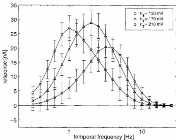
and double the signal amplitude. Device mismatch in the mirror introduced additional offsets, so it was not used in this design. We could in principle use both single-ended outputs, but that would require more wires routed through each pixel, which would consume more area.For the multiplier to work properly, the common-mode voltage of the lower inputs (V2 and Vb) must be lower than the common-mode voltage of the upper inputs (Vl and Va). Simulation results show that acceptable behavior is obtained with a difference of only 50 m V. In order to lower the dc level of the lowpass filter output, we lowered the source voltage of the output FET in the current mirror of the 9mC filter (see Figure 4.2b). By placing the vtilt bias a few tens of millivolts below
Vdd , we lower the dc output level by (Vdd - vtilt) / /'C. This source voltage "tilt" increases the time constant of the lowpass filter, but we can compensate by raising IT. The difference in source voltages also creates an asymmetry in the up-going and down-going slew rates of the filter, but in practice this does not seem to have a significant effect on the overall circuit performance.
It can be shown from Equation 4.2 that the circuit output saturates for differential inputs greater than about 4UT ~ 100 m V. Rather than restrict our signals to this small linear region, we exploit
the nonlinear behavior of the circuit to improve our motion detection algorithm. It has been shown that by adding saturating nonlinearities before the correlation stage, the contrast dependence of a Reichardt detector can be reduced (Egelhaaf and Borst, 1989). To understand this effect, consider Equation 4.2 in the extreme case where both differential inputs are much greater than UT :
where the sign function sgn(x) is defined as
1,
x>O
(4.5)
-1,
x<O
Incorporating this "saturated multiplier" model into our analysis from Chapter 3, we can rewrite Equations 3.15 and 3.16 as
m1 (t)
=
sgn [cos(ws¢+
P) - cos(2wtt - P)] (4.6)m2(t)
=
sgn [cos(ws¢ - P) - cos(2wtt - P)] (4.7)where P is given by Equation 3.18. We normalize for the constant prefactor in Equation 4.4 and neglect the constant dc component since the opponency subtraction will cancel this current.
We can continue the analysis of an EMD array with nonlinear multipliers by using the time averages of m1(t) and m2(t), which are given by
2
{m1 (t))
= 1 - -
(ws
¢+
tan-1 TWt) 7r2 (
- 1 )
(m2(t))
=
1 - - ws¢ - tan TWt 7rWhen these signals are subtracted in opponency, the time average of the output is given by
(o( t)) - tan-4 1 TWt 7r
4
- tan-1 TVWs 7r
(4.8)
(4.9)
(4.10)
Spatial integration across a small array of motion detectors will have the effect of integrating over different phases of the stimulus. This will remove the time-dependent components of the motion detector output.
We see in Equation 4.10 that in the limit of full multiplier saturation the output is sensitive to pattern velocity and spatial frequency but is independent of pattern contrast. Compare this to the original Reichardt motion detector response given by Equation 3.20, where the contrast dependence is quadratic. We use the inherent saturation in the Gilbert multiplier to achieve this behavior without adding additional hardware. We shall demonstrate this reduced contrast dependence in the following chapter.
Note that while we call this circuit a voltage-mode design, the final outputs of the EMD are two currents.
outlined in Figure 3.3b. All experimental results shown below were measured from arrays of this circuit, which was fabricated in a 1.2 /Jm double-poly, double-metal n-well CMOS process, yielding a pixel size of 61 /Jm x 199 /Jm with 32 transistors and a 4 capacitors totaling 3.0 pF. In order to build a 2-D motion sensor, we need add only two more multiplier circuits and additional interpixel and output wiring. Only two wires in each direction are required for nearest-neighbor communication, making 2-D layout practical. An additional interpixel wire may be required if opponent subtraction is performed locally.
While our fill factor is low (3.3%), we argue that fill factor is not an important factor for motion sensors. Defocused optics can be used to eliminate spatial aliasing. If low-light operation is required and catching every photon is essential, microlens technology currently used in CCDs could be used. All data shown was measured from an analog VLSI chip fabricated in a standard, commercially available 1.2 /Jm CMOS process. The 2.2 mm x 2.2 mm chip contained six parallel one-dimensional arrays of 24 EMD opponent pairs each with integrated photoreceptors (see Figure 4.4). Multiple rows of motion detectors are useful in practical applications because some rows may be focused on featureless parts of a scene. The outputs of all EMD pairs were summed to simulate the wide-field motion-sensitive neurons found in flies. We mounted a 2.6 mm lens over the chip, which gave the photoreceptors an angular spacing of 1.3° (similar to the 1 ° _2° angular spacing observed in fly eyes), and a total field of view of 30° (much less than the fly's eye, which sees almost an entire visual hemifield). The lowpass filter time constant was set to 50 ms, and the bandpass filters were set to pass frequencies between 0.5 Hz and 8 Hz.
4.2.2
Supply Voltage Requirements
By computing motion in parallel, we do not need time constants less than a millisecond at any pixel. The fastest known visual systems (those of houseflies) have bandwidths of less than 200 Hz, and humans can barely perceive the flicker of a 60 Hz monitor. This low bandwidth requirement allowed us to operate the entire circuit in subthreshold (drain currents typically less than 1 /JA). Subthreshold operation allowed us to operate at Vdd = 2.5 V despite the Gilbert multiplier circuit, where three transistors are in series between the power supply and ground.
25
4.2.3
Matching Considerations
Device mismatch is inherent in any physical circuit, and is an important consideration when designing analog circuits that will be repeated many times across a chip. We want every motion sensor on a die to exhibit similar performance. The large number of sensors on a single chip precludes off-chip trimming of each circuit to achieve matching. Some floating-gate circuits are capable of storing correction factors locally, but these would add to the size and complexity of each circuit (Harrison et al., 1998).
We use two types of devices in our EMD: transistors and capacitors. Parallel plate capacitors in CMOS, even very small ones, match very well (Minch et al., 1996a). In order to study transistor matching, we fabricated arrays of several hundred nMOS and pMOS transistors, and measured their matching characteristics.
Transistor mismatch is most simply modeled as a voltage source in series with the gate. This gate voltage variation is particularly important in subthreshold operation due to the increased relative transconductance in this region. \Ve modeled this source as a Gaussian distribution of mean zero and standard deviation (J. We estimated (J for nFETs and pFETs of various sizes by measuring I-V characteristics across the transistor arrays.
As expected, (J decreased with the square root of transistor area (data not shown). This behavior has been observed in other studies of subthreshold FETs (Pavasovic et al., 1994). We also found that the value of (J for pFETs was 2.7 times as large as the value for nFETs of equal gate area, on average.
We used a simple model for transistor mismatch:
(
(JOn
(In A) =
VA
(4.11)( 4.12)
where A is the gate area, and (Jop = 2.7(Jon ~ 31 mV"/tm in our technology (AMI 1.2 Mm 2-poly, 2-metal BiCMOS process available through the MOSIS fabrication service).
Using this knowledge, we can apportion our limited layout area in a way that maximizes interpixel matching. We analyzed sub circuits in our motion sensor to determine what effect variation in an individual device would have on the entire subcircuit. For example, analysis of the five-transistor lowpass filter (see Figure 4.2b) reveals that mismatch in each of four transistors-the two nFETs in the differential pair (M2 and M3 ) and the two pFETs in the current mirror (M4 and M5)-contribute equally to the inter circuit variance of the output voltage:
Given a limited area for circuit layout, it follows that to minimize mismatch, we must apportion the chip area as follows:
(4.14)
where Ap and AN are the layout areas devoted to pFETs and nFETs, N p and N N are the number
of pFETs and nFETs that contribute equally to the total circuit variance, and ap = 2.7an in our
technology. We used this consideration-allocating more area for pFETs due to their worse matching properties-when designing the layout. We also tried to reduce the total number of pFETs in the circuit (e.g., removing the pFET current mirror from the Gilbert multipliers).
Also, we drew transistors at least twice minimum width and three times minimum length to facilitate matching and reduce channel-length modulation effects.
a Photoreceptor b Temporal Derivative Circuit
.. f C dV.L
IBPF
positive component 0
dt'
+
P--< bias
Vphoto
. C
dV+~C
df
sf
negative component of C
~Y"
I
BPF-single EMD
c Low-Pass Filter
dlLPF
't
----cit
+
I LPF=
I BPFcUr
' t =
-l't
lout=
I
SPFI
LPFI
refI---r---'--Vreceptor
i(x,t)
p(t)
\
(a)
m(t)
lout
~
1 - - - - 1
I---r---r-Vout
I(t)
I
C'
(b)
(c)
Figure 4.2: Voltage-mode EMD subcircuits. Shaded labels indicate corresponding signals from Fig-ure 3.3a. (a) Adaptive photoreceptor (M1-M4 , C1-C2 ) with source follower (M5-M6 ) and temporal
highpass 9mC filter (M7-Mll , C3 ) to remove the dc component of Vphoto. (b) Temporallowpass
20
~m(33
A)
photodiode
adaptive
photoreceptor
temporal
highpass
filter
temporal
lowpass
filter
multipliers
Figure 4.3: Voltage-mode motion detector layout. Cell measures 61 f.Lm x 199 f.Lm in a standard
30
i
2.2
mm
I
silicon die
VLSI Motion Detector
Chapter 5
Characterization
The voltage-mode elementary motion detectors described in the previous chapter demonstrated
superior matching characteristics for similar pixel sizes. In this chapter, we characterize in detail the behavior of the voltage-mode EMD to both simple and complex visual stimuli.
5.1
Methodology
All of the experiments in this chapter were carried out on a 1 x 22 array of motion sensors fabricated on a 2.2 mm x 2.2 mm die in a standard 1.2 /lm CMOS process. A 2.6 mm focal length lens was mounted directly over the chip, giving a 35° field of view across the entire array. The angle ¢ between
adjacent photoreceptors was 1.5°, comparable to the eyes of many flying insects (Land, 1997). The
chip was biased to an appropriate operating range, and the bias settings were unchanged during all
experiments, except where explicitly stated.
For experiments involving spatial integration over many sensors, the individual output currents were summed on two wires, one for the rightward-facing half-receptors (i.e., the ml signal in Fig-ure 3.3a), and one for the leftward-facing half-receptors (i.e., the m2 signal in Figure 3.3a). The
currents were measured with off-chip sense amplifiers. The two opponent signals were subtracted to yield a direction selective response.
We presented computer-generated visual stimuli on a standard monitor (Sony Multiscan 17se II) with a refresh rate of 72 Hz (see Figure 5.1). Our software was able to update the screen at
approximately the same rate. The bandwidth of the adaptive photoreceptors was set sufficiently low to attenuate screen refresh artifacts by 20 dB. This also prevented the photoreceptors from responding to the 120 Hz signal in ac incandescent lighting.
We generated visual stimuli with spatial resolution far exceeding the motion sensor array reso-lution. We used a 64-value gray scale to generate sinusoidal gratings and other complex stimuli of varying contrasts.
5.2
Direction Selectivity
32
Osci Iloscope
or Computer
chip
output
voltage
computer-generated display
Figure 5.1: Chip testing methodology. We mounted a lens directly over the chip to focus an image on the photoreceptor array. Moving patterns were generated on a standard computer monitor. The temporal bandpass filters in each EMD blocked the 72 Hz refresh rate signal from the monitor.
array is highly direction selective, giving responses of opposite sign to motion in opposite directions. The individual sensor shows a high degree of pattern dependence superimposed on a dc direction selective response. Much of this pattern dependence is caused by device mismatch in the Gilbert multiplier. If the differential pairs are not perfectly matched, the output contains components of the raw input signals.
pattern velocity [deg/s]
_2
20~
U_m_mm ______ m_m_J
~'---.,---i
2 single photoreceptor output Vphoto [V] 1.8
1.6 1.4 5
o
-5 50
o
-50
o
2 4 6 8time [sec]
10 12 14
Figure 5.2: Direction selectivity. A sinusoidal grating (it
=
3.0 Hz,Is
= 0.14 cycles/degree [cpd], contrast = 1) moved along the motion detector axis in alternating directions. Spatial integration over an array of 22 Reichardt detectors eliminates much of the pattern dependence seen in the single sensor trace.5.3
Response to Simple Stimuli
The summed chip response (see Figure 5.2) was similar to the membrane potential of HS and VS cells, non-spiking wide-field motion-sensitive neurons in flies in three ways:
• Direction selectivity. The sign of the response indicates motion direction (Haag and Borst, 1997).
• Transient oscillations at motion onset. At the onset of stimulus motion, a large transient response oscillates with the temporal frequency of the stimulus pattern (see Figure 5.3). This transient decays to a steady state level at a rate given by the time constant of the EMD lowpass filter (approximately 50 ms) (Egelhaaf and Borst, 1989).
Cii
:0;
c:
Q)
-
oa.
Q)
c: co
....
.cE
Q)
~
34
12mvl _ _
~~_O_m_s._c ______________________ ~
4 Hz
L---8 Hz
16 Hz
_MOllon_
Time-Figure 5.3: Motion onset and offset responses in the fly's nonspiking HS interneuron. At the onset of stimulus motion, large transients oscillate with the temporal frequency of the stimulus pattern (indicated above each plot). The offset of stimulus motion produces no oscillations. (From Egelhaaf and Borst, 1989)
To further investigate the nature of the onset oscillations, we derived the transient response of the Reichardt motion detector at the beginning and end of motion. The analysis in Chapter 3 considered only the steady-state case. Following is the time-domain analysis for transient motion of a sinusoidal grating. Transient Reichardt motion detector responses have been derived for a simplified EMD model with no high pass filters in the photoreceptors to adapt away dc illumination (Egelhaaf and Borst, 1989). The addition of the highpass time constant greatly complicates the analysis, but significantly affects the response.