The use of visual angle in car following
traffic microsimulation models
AlObaedi, JTS and Yousif, S
Title The use of visual angle in car following traffic microsimulation models Authors AlObaedi, JTS and Yousif, S
Type Conference or Workshop Item
URL This version is available at: http://usir.salford.ac.uk/9686/ Published Date 2009
USIR is a digital collection of the research output of the University of Salford. Where copyright permits, full text material held in the repository is made freely available online and can be read, downloaded and copied for noncommercial private study or research purposes. Please check the manuscript for any further copyright restrictions.
The use of visual angle in car following traffic
micro-simulation models
Jalal Al-Obaedi1 and Saad Yousif1
1
Research Institute for the Built and Human Environment, University of Salford,
Salford, M5 4WT, United Kingdom
Email: [email protected]; [email protected]
Abstract:
This paper presents a detailed literature review on car following models and methods used in describing the behaviour between two drivers of successive vehicles travelling in a traffic stream. The paper then concentrates on presenting a proposed car following model based on visual information which are perceived by the driver of the following vehicle. The model represents a modified version of similar models used in the past for describing the “leader-follower” behaviour which depends on the use of visual angle in determining the required spacing between pairs of vehicles. A sensitivity analysis is carried out in order to find out reasonable horizontal angular velocity threshold values which give best representation of driver‟s reaction time. The capability of the model is then tested to represent the effect of size of vehicles on such threshold values and the required distance between vehicles. Further tests to calibrate and validate the proposed model are needed in order to represent real traffic behaviour using data from selected sites. The proposed model will mainly be used at a later stage in representing traffic behaviour at motorway ramp metering and measuring its effectiveness.
Keywords:
Car following, driver reaction time, traffic micro-simulation models, visual angle
1
Introduction
Car-following models describe the relationship between pairs of vehicles in a single lane. This relationship is represented by several mathematical models which basically describe the effect of the leading vehicle on its follower. The reaction of the driver of the following vehicle is expressed by his/her acceleration or deceleration depending on the leader‟s speed and the relative distance between the two vehicles.
2
Review of Car Following Models
Car following models are well described in the literature (see for example, Brackstone and McDonald (1999) and Panwai and Dia (2005)). These models can be classified into several groups as shown in the following sections.
2.1 Gazis-Herman-Rothery (GHR) Model
This is known as the GHR model. It represents the earlier car following model which was formulated in 1958 at the General Motors Research Laboratory in Detroit (Chandler, Herman and Montroll, 1958). According to the model, the acceleration/deceleration of the follower is based on relative velocity, relative spacing and the following vehicle‟s velocity.
Brackstone and McDonald (1999) provided detailed information regarding the choice of the model parameters for different researchers and stated that the GHR model is now being used less frequently because of the large number of contradictory findings for the values used to represent these parameters. Gipps (1981) reported that the model parameters have no explicit connection with drivers‟ or vehicles‟ characteristics.
2.2 Collision Avoidance Models (CA)
This is known as the CA model. The original formulation of this approach dates back to Kometani and Sasaki (1959). According to these models, a safe separation distance is assumed to be maintained between the follower and the leader.
Gipps (1981) introduced a car following model based on the assumption that the follower selects his/her speed to ensure that he/she can bring his/her vehicle to a safe stop should the vehicle ahead came to a sudden stop. According to Gipps, the minimum distance between two vehicles is affected by 1.5 times the driver‟s reaction time.
Benekohal and Treiterer (1988) developed a CAR following SIMulation model (CARSIM) to simulate traffic for both normal and stop and go conditions. Here, the acceleration/deceleration of the follower is based on the follower‟s desired speed and its engine capability. The model provides a minimum distance between the leader/follower which is equivalent to 1.0 times the brake reaction time.
Hidas (1998)reported that several researchers (e.g. Chen et al., 1995 and Parker, 1996) have found that the assumption of a safe distance is not obeyed by the majority of drivers. This meant that observations from real traffic conditions show that some drivers tend to have “close following” behaviour.
2.3 Desired Spacing Model
According to this model, the acceleration of the follower is a function of both relative distance and relative speed between the leader and follower. Also, it is a function of the desired following distance the follower wishes to maintain. The desired distance is a function of the speed of the follower.
2.4 Psychophysical Models
These models consider the ability of human perception of motion which assumes that the driver will accelerate/decelerate depending on a perceived threshold value. Basically, the perceived threshold is related to the difference in speeds or spacing between pairs of vehicles.
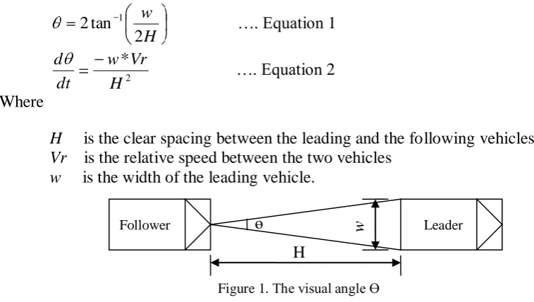
Visual angle models are described by researchers such as Brackstone and McDonald (1999) and Panwai and Dia (2005) as one type of psychophysical (or action point) models. Michaels (1963) observed that the detection of relative velocity depends on the rate of change of angular motion of an image across the retina of the eyes of the follower. The visual angle (ө) as shown in Figure 1 and its rate of change or angular velocity (dө/dt) are calculated as shown in Equations 1 and 2. Once the absolute value for this threshold (dө/dt) is exceeded, a driver notices that his/her speed is different from that of the vehicle ahead, and reacts with an acceleration/deceleration opposite in sign to that of dө/dt (Ferrari, 1988).
H w
2 tan
2 1 …. Equation 1
2
*
H Vr w dt
d
…. Equation 2
Where
H is the clear spacing between the leading and the following vehicles
Vr is the relative speed between the two vehicles
w is the width of the leading vehicle.
[image:4.595.114.493.280.494.2]
Figure 1. The visual angle Ө
According to Michaels (1963), the visual angle threshold ranges between 0.0003 and 0.001 rad/sec and it is reasonable to use 0.0006 rad/sec as an average value. Fox and Lehman (1967) described a car following model based on the visual angle concept using a base value of the threshold as used by Michaels (i.e. 0.0006 rad/sec). Ferrari (1989) presented a traffic simulation model for motorway conditions assuming that the angular velocity threshold to be identical for all drivers. He used a value of 0.0003 rad/sec with a minimum time gap between two successive vehicles of 1 second.
Hoffman and Mortimer (1994, 1996) carried out a study to scale the relative velocity between vehicles. They reported that when the rate of change of the subtended angle of a lead vehicle exceeds the threshold value (which is 0.003 rad/sec), drivers have the information available to subjectively scale the relative motion between two vehicles and drivers were able to give reasonable estimate of time to collision.
The second threshold is particularly relevant to close distance (spacing) headways where speed differences are always likely to be below the angular velocity threshold (Brackstone and McDonald, 1999). This is related to the well known Weber‟s law (according to this law, any change would be noticeable if it exceeds the just noticeable difference (JND) which is usually 10%). Therefore, a driver chooses to accelerate or decelerate in case the spacing is changed by a value of 10% of their desired spacing.
w
ө
Follower Leader
A comparative evaluation by Panwai and Dia (2005) applied on three micro simulation models namely, Verkehr in Stadten-simulation (VISSIM) and parallel microscopic simulation (PARAMICS) representing the psychophysical models and (AIMSUN) representing the collision avoidance model, has been made. The study showed that the first two models (i.e. VISSIM and PARAMICS) gave similar error values when tested using the same site data. These errors were found to be greater than those found using AIMSUN for the same set of data. Both VISSIM and PARAMICS are currently the main traffic simulation software used by industry in the UK for assessing transport impacts.
2.5 Other Car Following Models
There were several other attempts by researchers to model car following using alternative methods. The fuzzy system of the car following model describes a follower‟s response to the change of relative speed and headway to that of the leader according to his/her own free speed and desired safe following distance. The model divides the variables such as speed and headway into a number of overlapping sets associating each one with a particular term such as „close‟ and „very close‟.
Cellular automata models represent simple microscopic models which are straightforward with logic that usually consist of a few integer operations. According to Bham and Benekohal (2004), Nagal (1995 and 1998) reported that cellular automata models do not have realistic drivers and vehicle behaviour models. Because of a high computational resources and the long execution time in car following, Bham and Benekohal (2004) developed a cell based traffic simulation model called CELLSIM using a dual-regime constant acceleration model and two deceleration models. Space in the model was divided in cells of 1 ft (0.31m).
2.6 Summary of Limitations Associated with Existing Car Following Models
From the above brief review, some of the main limitations in car following models can be summarised as follows:
Most of the above models assign a pre-defined single value for each driver as his/her reaction time. Some researchers used two values for each driver to represent the alerted and surprised (not alerted) driver‟s reaction time for congested and non-congested traffic conditions, respectively. The majority of such models could not represent the follower‟s reaction time to show how it varies with traffic conditions.
The effect of the size of the leading vehicle on car following is not represented as a factor influencing the distance or time required between the leader and its follower.
In this paper, it is found (as will be discussed in detail later) that using psychophysical or action point models can easily deal with the above limitations, especially if the threshold values for the angular velocity are chosen appropriately.
3
Research Methodology
According to Kotsialos and Papageorgiou (2001) these models can be used for estimation, prediction and control related tasks for the traffic process. Moreover, computer simulation models can help in analysing everyday‟s traffic management needs by looking at problems such as congestion and identify their sources.
This section describes the proposed car following model which mainly depends on the visual angle perceived by the follower. The assumptions and the selected threshold angular velocity values for the proposed model are based on the sensitivity analysis tests which were carried out using Excel spreadsheets. This proposed model deals with the limitations presented in Section 2.6 above. The model was developed using Salford FORTRAN-95 in order to be used at a later stage in describing the behaviour at motorway merges.
3.1 Model Parameters
3.1.1 Threshold Values for Angular Velocity
The proposed model is mainly based on visual angular velocity thresholds. For each individual driver, there are two angular velocity thresholds. A positive threshold is for cases where the follower‟s speed is higher than its leader‟s speed. However, when the follower‟s speed is less than its leader‟s speed, a negative angular velocity threshold is applied.
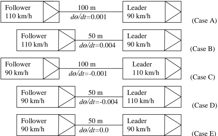
The sketch in Figure 2 gives examples of angular velocity values for different cases based on calculations from Equation 2. These values are either positive, negative or zero. For cases A and B the angular velocity is positive (i.e. when the velocity of the follower is higher than that of its leader), whereas cases C and D represent negative angular velocities. Case E gives a value of zero for the angular velocity when both leader‟s and follower‟s speeds are equal and is not a function of the distance between them.
(Case A)
(Case B)
(Case C)
(Case D)
[image:6.595.157.527.466.697.2](Case E)
Figure 2. Illustration of positive, negative and zero angular velocities
Follower 90 km/h
Leader 90 km/h 50 m
d
ө/
dt=0.0 Follower90 km/h
Leader 110 km/h 50 m
d
ө/
dt=-0.004 Follower110 km/h
Leader 90 km/h 50 m
d
ө/
dt=0.004Leader 110 km/h 100 m
d
ө/
dt=-0.001 Follower90 km/h
Leader 90 km/h 100 m
d
ө/
dt=0.001 Follower3.1.2 Time Headway Thresholds
If the angular velocity value is within the two threshold limits described above, the follower may choose to accelerate or decelerate depending on how close (clear time or distance) he/she is from his/her leader.
If the actual clear time between vehicles is less than the minimum time headway threshold (THmin), the driver will decelerate to reach his/her desired minimum spacing. If the maximum desired spacing threshold (THmax) is exceeded, the follower can accelerate to reach his/her desired speed. These desired minimum and maximum spacings may be obtained from site by monitoring close following drivers, over a section of a road, travelling with similar speeds.
3.2 Model Assumptions
The following assumptions are applied to calculate the acceleration of the follower: (a) If the positive angular velocity threshold is exceeded (i.e. d
ө/
dt from Equation 2is higher than the positive angular velocity threshold), the driver will decelerate with a minimum of the following two decelerations.
i) Maximum comfortable deceleration which is assigned for drivers. In emergency cases, the maximum deceleration rate should be used instead. ii) A deceleration which is enough for the follower to keep his/her vehicle
at a certain distance from the vehicle ahead. This distance is based on preferred time spacing for each individual driver.
(b) If the negative angular velocity is below the minimum negative threshold (i.e.
d
ө/
dt from Equation 2 is less than the negative angular velocity threshold), the driver will accelerate with a minimum of the following three accelerations. i) Maximum acceleration which depends on the engine capability of thevehicle.
ii) An acceleration to enable the follower to reach his/her desired speed. iii) An acceleration to enable the follower to perform his/her desired spacing
based on preferred minimum time spacing.
(c) If the angular velocity value is within the two visual angle threshold limits, the acceleration or deceleration of the follower is based on whether or not the follower exceeds the time headway thresholds (i.e. THmax and THmin) as discussed in Section 3.1.2.
(d) If none of the above thresholds are exceeded (i.e. angular velocity thresholds are as in (c) above and the time headway thresholds are within the minimum/maximum limits), the follower will keep a constant speed (i.e. acceleration is zero).
4
Model Applications
4.1 Modelling of Driver’s Reaction Time
4.1.1 Background Information on Reaction Time
Reaction time indicates a time lag that the follower uses to react to the change in his/her leader‟s driving behaviour during car following (Zhang and Bham, 2007). O‟Flaherty (1986) stated that the length of perception time varies considerably since it depends upon the distance to object, the natural rapidity with which the driver reacts, the optical ability of the driver and other factors.
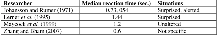
[image:8.595.106.545.335.409.2]Table 1 shows a summary of some of the main work in determining driver‟s reaction time. It is clear from the different trials to estimate driver‟s reaction time that there are some difficulties in doing so accurately. Maycock et al. (1999) reported that the key problem of estimating reaction times from driver‟s responses is that of identifying the start time from which the response should be measured. All researchers shown in the Table (apart from the last one) obtained the values of reaction time from experimental work where drivers were monitored individually on trial sites or in laboratory based experiments. The work by Zhang and Bham (2007) was based on analysing car-following trajectory data using Next Generation Simulation model (NGSIM).
Table 1. Summary of brake reaction time based on previous research Researcher Median reaction time (sec.) Situations
Johansson and Rumer (1971) 0.73, 054 Surprised, alerted Lerner et al. (1995) 1.44 Surprised
Maycock et al. (1999) 1.2 Unaltered Zhang and Bham (2007) 0.6 Not specific
4.1.2 Sensitivity Analysis of Brake Reaction Time
In this paper, the value of brake reaction time can be integrated within the proposed visual angle model parameters. This will eliminate the need to have brake reaction time estimated or measured from experimental work or likewise. Moreover, the proposed model represents the brake reaction time as a function of traffic density, relative speed, leader-follower acceleration/deceleration and other behaviours.
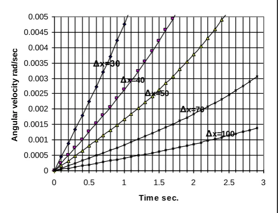
The driver‟s reaction time according to the proposed model is shown in Figure 3. The figure shows the relationship between relative angular velocity and time for different initial spacing between pairs of vehicles. The time is represented from the start of deceleration of the leader with a constant deceleration of -2m/s2. Also, 90 km/h speed is assumed for both of the leader and the follower.
The figure shows that when the traffic density is high (i.e. spacing is low), the follower will react to the deceleration of the leader within shorter times compared with the case of lower traffic density. For example, when the initial spacing is 40 m and for the case of threshold value of 0.003 as suggested by Hoffmann and Mortimer (1994, 1996), the follower will react to the leader‟s deceleration after 1.1 sec. Whereas for the case of 50 m initial spacing, the driver will react after 1.6 sec.
0 0.0005 0.001 0.0015 0.002 0.0025 0.003 0.0035 0.004 0.0045 0.005
0 0.5 1 1.5 2 2.5 3
Tim e sec.
[image:9.595.170.453.61.278.2]A n g u la r v e lo c it y r a d /s e c Δx=100 Δx=70 Δx=50 Δx=40 Δx=30
Figure 3. Relationship between angular velocity and time (assuming that leader‟s constant deceleration is equal to -2m/sec2 for different initial space headways)
0 0.5 1 1.5 2 2.5 3
30 40 50 60 70
Initial spacing (m )
D ri v e r re a c ti o n t im e ( s e c )
Threshold Hoffmann and Mortimer =0.003 rad/sec
Threshold by Michaels = 0.0006 rad/sec
Figure 4. Relationship between driver‟s reaction time and initial spacing
For relatively high density conditions (i.e. with spacings of say 40 m) Hoffmann and Mortimer‟s thresholds suggest that the reaction time is about 1.1 sec, whereas the threshold suggested by Michaels yield a value of reaction time of 0.2 sec. It seems that comparing these results with those in Table 1 based on previous literature, the threshold values of 0.003 as suggested by Hoffmann and Mortimer give more reasonable representation for angular velocity models. Therefore, in order to use the threshold values suggested by Michaels, there should be another parameter (namely an extra brake reaction time) which needs to be considered in modelling car following.
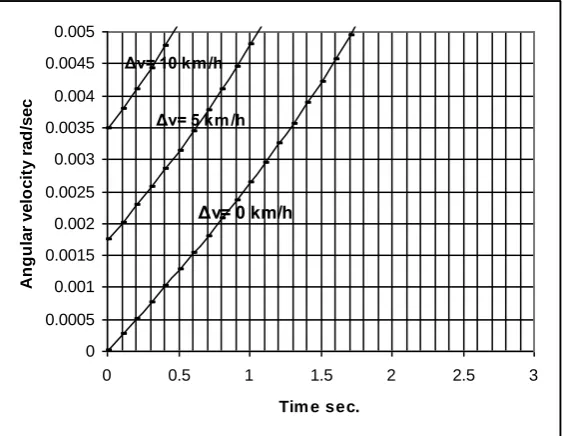
The modelling of driver‟s reaction time for different relative speeds is shown in Figure 5. The results are based on the same initial spacing of 40 m with assumed leader‟s speed of 90 km/hr (equivalent to 25 m/sec). The Figure shows that for a specific angular velocity threshold value, driver‟s reaction time decreases as the relative speed increases.
[image:9.595.181.470.315.454.2]
0 0.0005 0.001 0.0015 0.002 0.0025 0.003 0.0035 0.004 0.0045 0.005
0 0.5 1 1.5 2 2.5 3
Tim e sec.
A
n
g
u
la
r
v
e
lo
c
it
y
r
a
d
/s
e
c
Δv= 0 km/h
[image:10.595.180.462.60.278.2]Δv= 5 km/h Δv= 10 km/h
Figure 5. Relationship between angular velocity and time after leader‟s constant deceleration of -2m/sec2 for different relative speeds
4.2 Representing the Effect of the Size of Vehicles
Based on real data from UK motorway sites, Yousif (1993) reported that some passenger car drivers try to leave sufficient space to avoid visual problems associated with obstructed traffic signs or other traffic control devices on the road especially if they are in the vicinity of roadworks sites and close to exits at motorway junctions. This could contribute to forcing drivers following heavy goods vehicles (HGVs) to leave a much larger space. Parker (1996), when studying the effect of HGVs at three motorway roadwork sites, reported that the presence of HGVs in the traffic stream increases headways, thus reducing the capacity of the road section.
It was shown that most of other car following models, such as collision avoidance and desired spacing models, could not directly include the effect of the size of the leading vehicle. However it is interesting to refer to Yousif‟s (1993) assumption to include the effect of HGVs by assuming that when a car follows an HGV or when the follower vehicle is an HGV, the absolute maximum deceleration will be reduced by a certain value. This assumption led to having space headways for a Car following an HGV or an HGV following an HGV to be greater than the case of a Car following a Car.
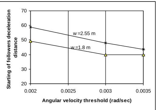
Visual angle models can also take into consideration the effect of the size of vehicles without making any further complicated assumptions. Figure 6 shows the effect of different widths of the leading vehicle on the starting distance for the follower to be affected by its leader. This is based on the assumptions that there is a 10 km/h relative speed difference between the two vehicles and with THmin and THmax equal to 1.6 and 2.0 seconds, respectively.
20 30 40 50 60 70
0.002 0.0025 0.003 0.0035
Angular velocity threshold (rad/sec)
S
ta
rt
in
g
o
f
fo
ll
o
w
e
rs
d
e
c
e
le
ra
ti
o
n
d
is
ta
n
c
e
[image:11.595.185.447.58.240.2]w =1.8 m w =2.55 m
Figure 6. Distance for the follower to be affected by its leader
5
Conclusion and Further Research
This paper presented a car following model which is based on visual angle using selected angular velocity threshold values (dө/dt). Several threshold values have been examined using sensitivity analysis. It was found that values of about 0.003 rad/sec (similar to those suggested by Hoffmann and Mortimer (1994, 1996)), gave reasonable results when testing the values obtained in representing driver‟s reaction time.
In addition, there was no need to introduce driver‟s reaction time as another parameter in the proposed model since it could be integrated within the selected angular velocity threshold values. This will eliminate the need to have brake reaction time estimated or measured from experimental work or likewise.
It was shown that the selection of 0.003 rad/sec threshold value gave reasonable results when the effect of the size of vehicles was to be considered in the modelling process. No further additional assumptions are needed if this threshold (or close to it) was selected.
For further work, it is important to examine the proposed model against real traffic data to test its validity for different traffic conditions (i.e. high to low densities with different operating speeds). The validated model will then be used in simulating traffic behaviour at motorway merges.
6
References
Aycin, M.F., Benekohal, R.F. (1998) Linear acceleration car-following model development and validation. Transportation Research Record 1644, TRB, Washington, DC, pp. 10–19
Benekohal, R.F., and Treiterer, J. (1988) CARSIM: Car-following model for simulation of traffic in normal and stop-and-go conditions. Transportation Research Board
1194, pp. 99-111.
Bham, G. H. and Benekohal, R.F. (2004) A high fidelity traffic simulation model based on cellular automata and car-following concepts. Transportation Research Part C,
Volume (12), pp. 1-32.
Brackstone, M. and McDonald, M. (1999) Car following: a historical review.
Chandler, R. E., Herman, R., and Montroll, E. W. (1958) Traffic dynamic: studies in car following. Operation Research, Volume (6), pp. 165-184.
Chen, S., Sheridan, T. B., Kusunoki, H. and Komoda, N. (1995) Car following- measurements simulation, and a proposed procedure for evaluation safety. Analyses, Design and Evaluation of Man-Machine System. Volume (2) pp. 529-34 Clark, J. and Daigle, G. (1997) The Importance of simulation Techniques in ITS
research and analysis. Proceedings of the 1997 Winter Simulation Conference. USA.
Ferrari, P. (1989) The effect of driver behaviour on motorway reliability.
Transportation Research Part B, Volume (23B), No. 2, pp. 139-150.
Fox, P. and Lehman, F.G. (1967) Safety in car following. Newark, (N.J.), Newark college of Engineering.
Gazis, D.C., Herman, R. and Rothery, W. (1960) Nonlinear follow-the-leader models of traffic flow. Research Laboratories, General Motor Corporation, Warren, Michigan, pp. 545-567.
Gipps, P. G. (1981) A behavioural car following model for computer simulation.
Transportation Research Part B, Volume (15) pp. 105-111.
Hidas, P. (1996) A car-following model for urban traffic simulation. Traffic Engineering and Control. Volume (39) pp. 300-305.
Hoffman, E.R. and Mortimer, G.R. (1994) Estimate of time to collision. Accident Analysis and Prevention, Volume (26), Issue 4, pp. 511-520.
Hoffman, E.R. and Mortimer, G.R. (1996) Scaling of relative velocity between vehicles.
Accident Analysis and Prevention, Volume (28), Issue 4, July 1996, pp. 415-421. Johansson, G. and Rumer, K. (1971) Drivers‟ brake reaction times. Human Factors,
Volume (13), No. 1, Feb., pp. 23-27.
Kometani, E. and Sasaki, T. (1959) Dynamic behaviour of traffic with non-linear spacing-speed relationship. In Symp. Theory Traffic Flow, Research Laboratory, General Motors, New York, pp. 105-109.
Kotsialos, A. and Papageorgiou, M. (2001) The Importance of traffic flow modelling for motorway traffic control, Networks and Spatial Economics, 1, Netherlands, pp. 179-203.
Lerner N., Huey R., McGee H. and Sullivan A. (1995) Older driver perception-reaction time for intersection sight distance and object detection, Report FHWA-RD-93-168, Federal Highway Administration, U.S. Dept. of Transportation, Washington DC. Maycock, G, Brocklebank, P. and Hall, R. (1999) Road layout design standards and
driver behaviour. Proc. Institution of Civil Engineers Transport, pp.115-122.
Michaels, R.M. (1963) Perceptual Factors in Car following. In Proceeding of the 2nd International Symposium on the Theory of Traffic Flow - OECD. pp. 44-59, Paris. Michaels, R.M. and Cozan, L.W. (1963) Perceptual and field factors causing lateral
displacements. Public Roads 32. pp. 233-240.
Nagel, K., (1995) High-speed micro simulations of traffic flow. PhD Thesis, University of Cologne, Germany
Nagel, K., (1998) From particle hopping models to traffic flow theory. Transportation Research Record 1644, Washington, DC, pp. 1–9
O‟Flaherty, C.A. (1986) Highways. Volume (1), Traffic planning and Engineering, 3rd Edition, Edward Arnold, London.
Panwai, S. and Dia, H. (2005) Comparative evaluation of microscopic car-following behaviour. IEEE Transactions on Intelligent Transportation System, Volume (6), No. 3, pp. 314-325.
Parker, M.T. (1996) The effect of heavy goods vehicles and following behaviour on capacity at motorway roadwork sites. Traffic Engineering and Control,
Wu, J., Brackstone, M. and McDonald, M. (2003) The validation of a microscopic simulation model: a methodological case study. Transportation Research Part C,
Volume (11), pp. 643-479.
Yousif, S. (1993) Effect of Lane Changing on traffic operation for dual carriageway roads with roadworks, PhD Thesis, University of Wales, Cardiff.