The Response of Prices to Technology
and Monetary Policy Shocks under
Rational Inattention
Paciello, Luigi
Einaudi Institute for Economics and Finance
23 November 2007
Online at
https://mpra.ub.uni-muenchen.de/5763/
Luigi Paciello
Northwestern University
November 2007
(Job Market Paper)
Abstract
The speed of in‡ation adjustment to aggregate technology shocks is substantially larger than to monetary policy shocks. Prices adjust very quickly to technology shocks, while they only respond sluggishly to monetary policy shocks. This evidence is hard to reconcile with existing models of stickiness in prices. I show that the di¤erence in the speed of price adjustment to the two types of shocks arises naturally in a model where price setting …rms optimally decide what to pay attention to, subject to a constraint on information ‡ows. In my model, …rms pay more attention to technology shocks than to monetary policy shocks when the former a¤ects pro…ts more than the latter. Furthermore, strategic complementarities in price setting generate complementarities in the optimal allocation of attention. Therefore, each …rm has an incentive to acquire more information on the variables that the other …rms are, on average, more informed about. These complementarities induce a powerful ampli…cation mechanism of the di¤erence in the speed with which prices respond to technology shocks and to monetary policy shocks.
1
Introduction
I present a model that is consistent with the empirical evidence that prices respond much more quickly to technology shocks than to monetary policy shocks. I show that this response pattern arises naturally in a framework based on imperfect information with an endogenous choice of information structure similar to Sims (2003). In my model, the only obstacle that
1 I am particularly grateful to Martin Eichenbaum, Giorgio Primiceri and Mirko Wiederholt for continous
…rms have when changing their prices is that they might not be well informed about the realizations of the shocks of the economy. The ability of a …rm to adjust its price quickly to a particular shock depends on how well informed the …rm is about the realization of that shock. The more attention a …rm chooses to pay to a given shock, the more informed the …rm is about the realizations of that shock. Similar to Sims (2003), I assume there is a limit on the total attention the …rm can pay to the di¤erent shocks impacting on the economy. Therefore, if the …rm allocates more attention to technology shocks, it must allocate less attention to monetary policy shocks. In my model, the …rm will optimally choose to allocate more attention to those particular shocks that most reduce pro…ts when prices are not adjusted properly. Since technology shocks a¤ect pro…ts more than monetary policy shocks, the …rm will allocate more attention to technology shocks than to monetary policy shocks.
Other things being equal, this e¤ect helps to rationalize the observed di¤erential speed with which prices respond to technology shocks and to monetary policy shocks. However, this e¤ect alone is not large enough to quantitatively account for the di¤erential response. Fortunately, complementarities in price setting generate complementarities in …rms’ decision
about which information to acquire1. These complementarities induce …rms to acquire and
process more information on the same variables that other …rms are more informed about. The reallocation of attention in favor of technology shocks, and away from monetary pol-icy shocks, generates a large ampli…cation in the di¤erence with which prices respond to technology shocks and to monetary policy shocks.
I choose the parameters governing …rms’ information processing capabilities such that the loss each …rm faces from not being perfectly informed is a very small fraction of prof-its. The degree of strategic complementarity in price setting in my model is similar to the degree of strategic complementarity in price setting generally adopted in the large literature investigating the implications of price stickiness for the dynamics of macroeconomic
vari-ables2. As it turns out, under my assumptions, …rms respond to technology shocks roughly
as they would under complete information. In contrast, …rms respond much more slowly to monetary policy shocks than they would under complete information.
There is a large empirical literature investigating how macroeconomic variables respond to monetary policy shocks. In this literature, there is substantial consensus that in‡ation
1Hellwig and Veldkamp (2007) theoretically study the role of strategic complementarities in information
choices.
responds slowly to monetary policy shocks3. A more recent literature investigates the e¤ects
of technology shocks using structural vector autoregression (SVAR) models. Papers in this
literature consistently …nd that prices respond in general very quickly to technology shocks4.
Paciello (2007) studies the di¤erential speed in the adjustment of prices to technology and monetary policy shocks in the context of SVAR models using a variety of alternative iden-ti…cation schemes, sub-samples, and data from di¤erent countries. I show that the basic …ndings of the SVAR literature with respect to the di¤erence in the speed with which prices respond to technology shocks and monetary policy shocks are very robust. The same pat-terns that hold for the United States also hold for Canada, France, Japan, and the United Kingdom. I argue that the SVAR results for the United States re‡ect a negative, and statis-tically signi…cant, correlation between quarterly aggregate total factor productivity growth and di¤erent measures of aggregate in‡ation.
The di¤erent speed with which prices respond to technology shocks and to monetary policy shocks is not easy to reconcile with existing models of price stickiness. For instance, Smets and Wouters (2003, 2007) estimate a large-scale dynamic stochastic general equilib-rium model with many nominal and real frictions, using U.S. and European data. In their paper, sticky prices are modeled using Calvo style time-dependent contracts. Smets and Wouters (2003, 2007) …nd that the response of prices to technology shocks is very similar to the response of prices to monetary policy shocks, in terms of speed of adjustment and persistence. In a related literature, other authors model nominal frictions as arising from
the presence of menu costs5. These costs generate state-dependent pricing. In these
mod-els, …rms can adjust prices any time they wish by paying a menu cost. To the best of my knowledge, the impact of menu costs has not been analyzed in an environment where there are both aggregate technology shocks and monetary policy shocks. In general, the frequency of response of prices to technology shocks will be large if these shocks are large. Once …rms have paid the menu cost, they can adjust prices to all realized shocks. Therefore, if …rms ad-just prices very frequently to aggregate technology shocks, they will most likely adad-just prices frequently to monetary policy shocks. Menu costs models would then have a di¢cult time in accounting for the di¤erent speed with which prices respond to technology and monetary policy shocks.
3See for example Christiano, Eichenbaum and Evans (1999).
4See for example Shapiro and Watson (1998) or Altig, Christiano, Eichenbaum and Linde (2005). 5See for example Gertler and Leahy (2006), Golosov and Lucas (2006), Midrigan (2006), Nakamura and
The model I propose is related to Woodford (2002). Woodford (2002) uses an incomplete information model to explain the sluggish response of prices to nominal shocks. He argues that such a framework could potentially deliver a di¤erential response of prices to aggregate supply shocks relative to nominal demand shocks, if …rms were relatively more informed about the former than they were about the latter. However, he leaves open the question of why …rms should choose to be relatively more informed about some shocks. Sims (2003) and Mackóviak and Wiederholt (2007) study the endogenous optimal choice of the infor-mation structure. In particular, Mackóviak and Wiederholt (2007) focus on the di¤erential response of prices to aggregate nominal shocks versus idiosyncratic shocks in a framework with limited information-processing capabilities, and with an exogenous process for nominal spending. Firms use signals to set prices, but in their paper the signals are endogenous. Firms decide to be relatively more informed about idiosyncratic shocks because the latter have a larger impact on the pro…t-maximizing price. Furthermore, when …rms pay limited attention to aggregate conditions, there is a lower incentive for other …rms to pay attention to aggregate conditions. The model I propose di¤ers from Ma´ckoviak and Wiederholt (2007) in at least two dimensions. The …rst di¤erence is that I introduce two types of aggregate shocks. This assumption has important consequences, as it allows me to not only provide an explanation for the di¤erential speed of adjustment of prices to such shocks, but it gen-erates a large di¤erence in the allocation of attention by price setters across shocks through complementarities in price setting. The second di¤erence is that I embed the attention allo-cation problem in a more standard general equilibrium framework that captures the roles of di¤erent actors in in‡uencing the di¤erential responses of prices, with particular emphasis on the central bank.
2
Facts
Paciello (2007) investigates in details the responses of aggregate prices to monetary policy and technology shocks using SVAR models. Here, I report the results from the benchmark estimation procedure for the U.S. economy. I use a SVAR methodology to document the responses of aggregate prices to total factor productivity (TFP) shocks and monetary policy shocks. To this aim, I consider the following reduced form VAR:
Yt = (L)Yt 1+ut;
where Y contains all the variables of interest, and (L) is a lag operator of order p. The
covariance matrix of the vector of reduced-form residuals, ut; is : The variables I include
in the benchmark speci…cation are the growth rate in labor productivity, the Federal Re-serve Funds rate (FFR), the GDP de‡ator in‡ation, commodity in‡ation, the logarithm of per-capita hours worked, the logarithms of the ratios of consumption and investment to out-put, the logarithm of money velocity and the logarithm of labor productivity adjusted real
hourly wages6. In this speci…cation, the Federal Reserve Fund rate is the monetary policy
instrument, although results hold for other choices of instruments too. The sample period is
1959:2 - 2007:27 and, based on the Akaike criterion, I choose the number of lags to be four,
even if results are robust to di¤erent choices. Identi…cation in the structural VAR litera-ture amounts to providing enough restrictions to recover the decomposition of the estimated matrix of variance covariance of the reduced form VAR:
=A0A00:
From this relationship and imposed restrictions, there is a unique mapping from ut to the
vector of orthogonal structural shocks, t; such that ut =A0 t: Once this map is de…ned, it
6This speci…cation is similar to the one used by Altig, Christiano, Eichenbaum and Linde (2005), Francis
and Ramey (2005). Results would be unchanged to more parsimonious speci…cations.
7The following variables were obtained from DRI Basic Economic Database. Nominal gross output is
mea-sured by GDPD, real gross output by GDPQ. Nominal investment is GCD (household durables consumption) plus GPI (gross private domestic investment). Nominal consumption is measured by GCN (nondurables) plus GCS (services) plus GCE (government consumption). Per capita hours worked are measured by LBMNU (Nonfarm business hours) divided by P16 (US population above 16). Real wages per capita are measured by LBCPU (nominal hourly non-farm business compensation) divided by the price index and P16. The price index is GDP/GDPQ. Commodity price index is an index over commodities available from DRI.
is possible to estimate the series of structural shocks and the responses of the variables into the system to such shocks. Since I am interested in two structural shocks, I only need to
give conditions to de…ne the mapping fromutto the neutral and monetary policy technology
shocks. I identify the column of A0 relative to the neutral technology shocks through long
run restrictions as in Gali (1999), using a property of standard neoclassical models, where the only type of shock having an impact on labor productivity in the long run is a permanent
technology shock. The column of A0 relative to the monetary policy shocks is identi…ed
as in Christiano et al (2003), relying on the assumption that the Federal Reserve set the monetary policy instrument after some other variables have been realized. This means that
there is a subset of variables in Y; the ones in the Federal Reserve’ feedback rule, to which
the monetary policy shock is orthogonal. I therefore assume that all variables in the VAR enter the feedback rule except for the velocity of money.
The results presented in F igure 1 show that a positive TFP shock has a sudden impact
on the GDP de‡ator, with in‡ation dropping contemporaneously to the shock and then quickly converging to zero. In particular, a one basis point increase in TFP reduces prices on impact by approximately 0.35 basis points. The two standard deviations error bands con…rm that this result is signi…cant at a 5 percent signi…cance level. On the inverse, the GDP de‡ator responds very slowly to a FFR shock, with the peak of the response taking place approximately twelve quarters after the shock. In particular, following a negative one basis point shock to the FFR, we have to wait approximately six quarters before in‡ation is positive and statistically di¤erent from zero. But even then, the magnitude of in‡ation
is no larger than 0.08 basis points. Table 1 contains the variance decomposition of the
forecast error for in‡ation in terms of fractions of total variance. The …rst result is that the TFP shock accounts for most of the variance of the forecast error of in‡ation for the …rst 10 quarters. The second is that on the inverse the monetary policy shock explains a marginal proportion. Hence technology shocks are a much more important determinant of the volatility of in‡ation than monetary policy shocks.
3
The model economy
I introduce a dynamic general equilibrium model with three types of actors: households, …rms and central bank. Since I am interested in …rms’ price-setting behavior, I assume that these have limited information processing capabilities of the type suggested by Sims (2003).
For tractability, I assume that households and central bank have complete information8.
Households choose consumption, bond holdings, investments in physical capital, amount of working hours and capital services to supply to …rms. The central bank sets nominal rates following a Taylor type rule. There is a constant return to scale production function common to all producers, which use labor, capital and intermediate inputs as factors of production. The only two exogenous shocks are an aggregate neutral technology shock and a monetary policy shock.
3.1
Households
The household side of the economy is modeled along the same lines as that of Smets and Wouters (2007). Households have complete information. They maximize expected dis-counted utility given by:
E0
1
X
t=0
t
ln (Ct bCt 1) 0
1 + l L
1+ l
t ; (1)
where 2 (0;1) is the discount factor, Ct is the households aggregate consumption, Lt
denotes the household supply of labor, b is the coe¢cient de…ning the degree of habit
per-sistence in preferences, 0 and l determine respectively the level and the convexity of the
disutility of labor. A complete set of Arrow-Debreu contingent securities,Vt+1(!);is traded
in the economy. The household budget constraint and the technology to accumulate capital
at period t can be written as:
PtCt+
Bt
Rt
+PtIt+
Z
gt(!)Vt+1(!)d! (2)
= Bt 1+PtWtLt+Pt rtkut (ut) Kt+Vt+Pt t;
Kt+1= (1 )Kt+ 1 S
It
It 1
It; (3)
8Adams (2007) uses similar assumptions of complete information on households and central banks to study
whereKtis the stock of physical capital at the beginning of periodt,utis the capital utiliza-tion rate so that utKt is the total service of capital at time t; It is the level of investments,
Rt is the gross nominal interest rate on the risk free bonds Bt, Wt and rtk are respectively
the real wage and the rental rate of capital in period t, t is the dividend received from full
ownership in the …rms,Pt is the price of the unique …nal good of the economy andgt(!) is
the set of prices of state contingent securities. The functionS ItIt1 represents the
installa-tion (disinstallainstalla-tion) costs associated with accumulating (decumulating) stock of capital, and
similarly to Altig, Christiano, Eichenbaum and Linde (2005) satis…esS(1) =S0(1) = 0;and
S00(1) > 0. This captures the idea that installation costs are smaller for smoother growth
rates in investments9. The cost of capital utilization is captured by the function (u
t). As
in Smets and Wouters (2007), I assumeut= 1and (ut) = 0on the non-stochastic balanced
growth path.
Knowing the history up to timet, the household chooses the quantitiesfCt; Bt; It; Kt+1; Lt; utg
and the optimal holdings of state contingent securities,Vt+1(!);so to maximize the expected
discounted utility in (1) subject to(2) (3).
The composite …nal good, Yt; is a Dixit-Stiglitz aggregator over the set of di¤erentiated
goods indexed by z;
Yt=
Z 1
0
Yt(z)
1 1
; (4)
where is the elasticity of substitution across di¤erent varieties. I assume that Yt is
ag-gregated by the household and can be used indi¤erently for consumption, investments or production as an intermediate input.
3.2
Monetary Policy
The monetary policy authority sets short term nominal interest rates,Rt;following a Taylor
type rule described by:
Rt
R =
Rt 1
R
r 1 +
t
1 +
1 +yt
1 +y y
e"rt; (5)
9Although capital adjustment costs do not play any role in the di¤erential response of prices to the two
aggregate shocks, they turn out to be important in order to have a drop in nominal rates,Rt; following a
where "rt N(0; 2r) is the iid shock to the policy rule, R and are the non-stochastic
steady state values of nominal interest rates and in‡ation, t is the in‡ation rate at t, yt is
the growth rate in real value added output10 at time t, and y is the non-stochastic steady
state value of output growth. Orphanides (2003b) has shown that a rule speci…ed in terms of output growth is at least as well representative of the actual monetary policy in the United
States as a rule speci…ed in terms of output levels11. The reliance of information regarding
growth rates, as opposed to natural-rate gaps, is also consistent with verbal descriptions of policy considerations and is easy to communicate, since output growth rates are usually used to describe the state of the economy. Orphanides and Williams (2003, 2006) also show that the rule expressed in terms of growth rates in output is to be preferred to the rule expressed in terms of levels of output, when the state of the economy, and, in particular, potential output are unknown. In such a case, a rule speci…ed in di¤erences reduces the volatility of in‡ation and output induced by errors in the perception of the output gap. Related to this argument is the fact that I am assuming the central bank has complete information, which means it perfectly observes current output growth and in‡ation. If I were to model the rule depending on the levels, I should have scaled the potential output level by the state of technology in order to have a stationary output gap, as in my model there is a non-stationary stochastic component of the technology process. In that case, assuming complete information on the side of the central bank would have implied that the central bank perfectly knows the current state of technology, which is arguable as sustained by Orphanides and Williams (2003, 2006). In contrast, the speci…cation in terms of output growth requires the central bank to only observe current in‡ation and output growth, and to know their steady state values, which is equivalent to estimate a time trend. I believe that it is realistic to assume a central bank has enough information processing capabilities to implement such a rule.
3.3
Modeling the limited information capability
Here I introduce the tools used in this paper to model the limited information capability of …rms. I need to de…ne a measure to quantify the reduction in uncertainty coming from
10Real value added output is the sum of real aggregate consumption and investment,C
t+It:
11For example, similar to Justiniano and Primiceri (2005):
Rt
R =
Rt 1
R
r 1 +
t
1 +
Yt At
y
information processing. I build on the seminal work of Sims (2003) and use the concept of entropy to measure uncertainty in economic models. The larger is the entropy of a random
variable, the larger is the uncertainty about its realizations. The entropy H of a stationary
multivariate normally distributed random variable, xT = (x1; x2; :::xT);equals:
H(xT) = 1
2log2
h
(2 e)T j xTj
i
;
wherej xTj is the determinant of the variance-covariance matrix ofxT. Therefore, a normal
random variable has an entropy that depends only on the second moments of the distribution.
Close to the de…nition of entropy is the de…nition of conditional entropy ofxT = (x
1; x2; :::xT) given sT = (s
1; s2; :::sT) :
H(xT jsT) = 1
2log2
h
(2 e)T xTjsT
i
;
wherexT andsT must have a joint multivariate normal distribution, and where
xTjsT is the
determinant of the conditional-covariance matrix ofxT givensT:I then de…ne the reduction
in uncertainty about a vector of multivariate normally distributed random variablesxT;from
observing a vector of multivariate normally distributed random variablessT;as the di¤erence
between the entropy of xT and the conditional entropy of xT given sT :
I(xT;sT) = H(xT) H(xT jsT):
This measure is called mutual information. I can then de…ne the information ‡ow between two stochastic processes as the average per period amount of information that one process
contains about another process. If xT and sT are the …rst T realizations of the processes
fxtg and fstg;then the information ‡ow can be de…ned as:
I(fxtg;fstg) = lim
T!1
1
TI(x
T
;sT): (6)
In this paper, restricting information processing capabilities means restricting the average
information processed by an agent per period. The information ‡ow de…ned in (6) is the
measure used for it. In the case of stationary multivariate normally distributed random variables the information ‡ow reduces to:
I(fxtg;fstg) = lim
T!1
1
T log2
j xTj
xTjsT
!
;
and it is independent of the realizations of the signal process. When the process fstg is
is a constant, the conditional variance-covariance matrix is identical to the unconditional
one, and the implied information ‡ow is zero. When the process fstg is perfectly revealing
about the realizations of fxtg; there is no more uncertainty about the latter, and xTjsT
is zero, implying an in…nite information ‡ow. A process fstg that is not fully revealing,
but contains some information about the realization of fxtg will imply a …nite and strictly
positive information ‡ow.
3.4
Firms
There is a continuum of Dixit-Stiglitz monopolistically competitive …rms of mass one, and
indexed byz. Each …rm specializes in the production of a di¤erentiated product. Like Basu
(1995) and Nakamura and Steinsson (2007)12, I assume that all products serve both as …nal
output in consumption and investments, and as intermediate inputs into the production process of other products. Incorporating intermediate inputs into the production function increases the degree of strategic complementarity in price setting. Being that prices of intermediate inputs are directly linked to the aggregate price, the rigidity of prices to shocks is therefore ampli…ed and transmitted to …rms through rigidity of intermediate inputs prices. In
this structure, there is no …rst product that is made without the use of other products13. Each
…rm z uses an index of intermediate inputs, Xt(z); for production, which is, for simplicity,
assembled by the household as in(4). The production function of …rm z is then:
Yt(z) = At Kt(z) Lt(z)1
1
Xt(z) ;
whereYt(z)is the gross output of …rmz, At is the aggregate productivity variable common
to all …rms, which follows an exogenous stochastic process de…ned by:
lnAt+1
At
= a+ aln
At
At 1
+"at+1; (7)
12Basu (1995) and Nakamura and Steinsson (2007) apply this structure to a menu costs type model,
obtaining a high degree of strategic complementarity in price setting. Furthermore, Nakamura and Steinsson (2007) show that this type of complementarities is well suited to explain the high rigidity of aggregate prices to demand shock, and the high frequency of price changes due to idiosyncratic productivity shocks.
13As sustained by Basu (1995) this is well representative of the U.S. economy: ”Input-output studies
where "at+1 is normally distributed, "at+1 N(0; 2a); and is iid over time. Kt(z) is the
amount of capital services rent from households, andLt(z) is the labor input hired from the
households by …rmz. Total demand for good z; Yt(z); is:
Yt(z) = Yt
Pt(z) Pt
;
where aggregate demand, Yt; is:
Yt=Ct+It+
Z 1
0
Xt(z)dz+ (ut)Kt:
Each …rm has three decisions to take at each period t. The …rm has to choose the optimal
price, Pt(z), at which it is willing to sell any quantity demanded, and the optimal mix
of inputs, both in terms of ratio of capital to labor, kt(z) KtLt((zz)); and in terms of ratio of intermediate inputs to the other factors of production, xt(z) Kt(z)XtLt(z()z)1 . I assume
there are three separate decision makers at each …rm, one responsible for the choice of the selling price, one responsible for the optimal capital-to-labor ratio and one responsible for
the intermediate-inputs ratio14. For tractability, the …rm is not choosing the optimal basket
of intermediate inputs, Xt(z); which is assembled by the household15 as in (4). Formally
the problem of the price setter in each period t; at the …rmz; is choosing Pt(z) so to solve:
max
Pt(z)E
" 1 X
=t
(P (z); k (z); x (z); )jstzp
#
(8)
where is the discount factor16 between period t andt+ , andst
zp =fszp;1; szp;2; ::::; szp;tg
denotes the realization of the signal process up to timetfor the price setter at …rmz. Finally,
t = Yt; Pt; At; Wt; rtk is the vector of realizations of the aggregate variables outside the
control of …rmz. The optimization problems of the other two decision makers are similar and
therefore reported in appendix A. Up to this point, the decision problem at …rm z is quite
standard. Each agent makes an optimal decision conditional on its information set. If the information set contained all the realizations of current and past variables in the economy,
14This assumption is similar to the one used by Mankiw and Reis (2006). They assume that at each
…rm there is a price setting agent with incomplete information and an input decision maker with complete information. One di¤erence is that I allow for incomplete information for each decision maker at each …rm, but do not allow incomplete information on the household side.
15An equivalent assumption would be that there is a separate decision maker at each …rm that assembles
the basket of intermediate inputs in complete information.
16
we would be in the conventional case considered in the literature on monopolistically com-petitive …rms applied to macroeconomic models: …rms would price with constant markups to nominal marginal costs, and the optimal input choice would be de…ned by the relative price of production factors. In such a case, it would make no di¤erence whether there are three separate decision makers or only one, as choices are made on the basis of the same information set. In this paper, the information sets are endogenous. The optimal signal
process fszp;tg is chosen by the price setter in period zero and satis…es a constraint on the
average ‡ow of information,
I
n
Pa;ty (z); P
y
r;t(z)
o
;fszp;tg p (9)
where nPa;ty (z); P
y
r;t(z)
o
is the vector of stochastic processes for the complete information optimal responses to the two aggregate shocks. The sum of these two processes delivers
the optimal complete information price level, Pty(z) =P
y
a;t(z) +P
y
r;t(z). Therefore P
y
t (z)is
the price level the price-setter at …rm z would choose if she had complete information, or
equivalently if p !+1. In addition to choosing the price level at any period t, in period
zero the price setter at …rm z solves the following problem:
max
fszp;tg2SE
" 1 X
t=0
t (Pt (z); kt(z); xt(z); t)
#
(10)
subject to (9); where Pt (z) solves (8) at each periodt. The attention allocation problems
for the other two decision makers are similar and reported in appendix A.
The three decision makers at each …rm are indexed byj =p; k; x;indicating respectively
the price setter, the decision maker for the capital-to-labor ratio and the decision maker for
the intermediate-inputs ratio: Each decision maker is endowed with information processing
resources that allow her to process on average j bits of information per period17. The
allo-cation of j across separate decision makers is optimal, in the sense that the marginal value
of additional information across the three agents at each …rm is identical, and = Pj j
is the total of information-processing resources at each …rm; is chosen so that the overall
marginal value of information at the …rm level is very small18, implying a relatively small
17In information theory, the ‡ow of information is measured in bits. One bit is the ‡ow of information
necessary to completely reduce uncertainty about the realization of a discrete random variable with two equally likely outcomes. See Cover and Thomas (1991) for more details.
18In principle it would be an easy exercise to set up a cost function, or a market for information processing
friction: …rms would invest very few resources to acquire more information processing capa-bilities at the equilibrium. Intuitively, my model is equivalent to an organization structure where there are three separate managers at each …rm, a marketing manager in charge of the price choice, a production manager in charge of the optimal mix of capital and labor, and a purchasing manager, responsible for the optimal level of intermediate inputs relative to the other factors of production. On top of the three managers, there is a CEO that
allo-cates optimally the …rm total information processing resources, ;across the three managers
in period zero. Each decision maker uses its information processing capability to acquire and process information on those variables that most matter for its choice. Although each decision maker maximizes the same pro…t function, the optimal choice of the variable she is in control of, depends potentially on di¤erent factors. For example the decision maker in charge of the price level has to process information on the impact its choice has on the relative demand of the …rm. On the inverse, the two decision makers for the capital labor and intermediate-inputs ratios do not need direct information on demand, as they minimize the cost of production for any level of demand. I believe that the decision process at the …rm level is a complex activity that involves many individuals, each of them in charge of
a piece of the decision process19. Therefore distributing the decision powers across several
individuals seems more realistic.
3.5
Restrictions on the set of signals for the benchmark model
I assume that signals cannot contain information about future realizations of shocks, "a
t and
"r
t: This removes any forecasting power over shocks that have not yet been realized. This
assumption is not controversial as long as exogenous shocks are assumed to be independent over time, and this is the case for this paper. Second, I restrict the signals to follow stationary Gaussian processes:
fszj;t; "at; " r
tg is a stationary Gaussian process. (11)
This assumption allows having a closed form expression for the information ‡ow and facil-itates the computation of a solution for the optimal signal structure, as it reduces to the
19Zbaracki, Levy and Bergen (2007) study the decision process for a price cut at a large manufacturing
choice of variance-covariance matrices20. I assume that …rms acquire and process information
about the two types of shocks separately. This means that the signal …rmz receives at time
t is a vector that can be partitioned into two subvectors, one containing information about
f"atgand one containing information about f"rtg:
fszja;t; "atg and fszjr;t; "rtg are independent. (12)
This assumption is probably extreme, as in reality the two processing activities may have some overlapping, and hence there might be some learning about one shock by processing information about the other. I will relax this assumption later in the paper and show that not only results do still hold, but they are actually reinforced. Finally, I assume that all the noise in the signal is idiosyncratic, conveying the idea that all the information is available but the limited information processing capability generates idiosyncratic errors in the processing of available information.
3.6
Markets clearing conditions and resource constraint
In equilibrium, the markets for labor, capital and intermediate goods clear in each period
t: i) Lt =
R1
0 Lt(z)dz; ii) utKt =
R1
0 Kt(z)dz; iii) Xt =
R1
0 Xt(z)dz: Also, the bonds and
state contingent securities markets clear at each period t and state ! : Bt = 0; Vt(!) = 0:
Finally, the resource constraint is satis…ed in any period t:
Yt=Ct+It+Xt+ (ut)Kt: (13)
4
The solution to the static version of the model
In this section I solve a static version of the model introduced in section 3. This will provide useful insights and intuitions into how the attention allocation determines the dif-ferential speed of adjustment of prices to the two aggregate shocks, and how complemen-tarities and monetary policy a¤ect the responses of prices to these shocks. I impose
20When the objective function is quadratic, this assumption is not binding, because Gaussian signals turn
equal to zero, so that labor and intermediate inputs are the only inputs in production:
Yt(z) = AtLt(z)1 Xt(z) . I also assume that the decision maker choosing the optimal
intermediate-inputs ratio, xt, has complete information. Therefore in this economy only the
price setter faces an attention allocation problem. I impose thatAt isiid, hencelnAt="at:I
also assume no habit persistence in the utility function,b= 0:Finally, I restrict the monetary
policy rule to be static, assuming r = 0; and to take the form:
Rt
R =
Pt
P
Ct
C y
e"rt;
where Ct is aggregate demand and coincides with real value added output, and the rule
targets the deviation of the price level from steady state. I solve the model through a log-linearization around the non-stochastic steady state. The solution procedure for the attention allocation problem has two steps. In the …rst step I formulate a guess for aggregate prices and I solve for the dynamics of the model implied by the guess. In the second step I solve the attention allocation problem of the price setter, aggregate prices over …rms, and then solve
for the guess. The log-deviation of aggregate prices from steady state at time t is a linear
function of the realizations of two iid shocks at time t; which are the sole state variables21:
^
Pt= r"rt + a"at:
The optimal price of …rm z under complete information in log-deviations from steady state
is given by:
^
Pty(z) = ^Pt+ ^Ct (1 + l)" a
t; (14)
where = (1 + l) (1 ) is the degree of strategic complementarities in price setting, as
de…ned in Woodford (2003)22, andC^
tis the log deviation of real demand from steady state23.
A larger share of intermediate inputs in total costs, ; implies a larger degree of strategic
complementarity in price setting. Given the guess for aggregate prices and the solution for ^
Ct in terms of the two fundamental shocks, I obtain a linear equation that links the log
deviations of complete information optimal price, P^ty(z);to the two fundamental shocks:
^
Pty(z) = 1
1 + 1 + y
r+#r "rt+ 1
1 + 1 + y
a+#a "at; (15)
where #r = 1+
y; and #a = 1 : The shock "
i; i = a; r, has an impact on the complete
information price directly through parameter #i; and indirectly through the feedback from
aggregates prices. The magnitude of the latter is determined by the degree of strategic complementarities in prices, and the monetary policy rule. A larger degree of strategic
complementarities, a lower ;implies everything else equal a larger feedback from aggregate
prices. This is intuitive as more complementarities in price setting imply that the action of each price setter is in‡uenced more by the average action of the other price setters.
In order to solve for the attention allocation problem in (10); I take a log-quadratic
approximation of the sum of the discounted expected pro…ts in (10), expressed in terms of
log deviations from steady state. The optimal allocation of attention problem reduces to24:
min
fszp;tg2S!1E
^
Pt (z) P^
y
t (z)
2
(16)
s:t:
i) : P^ty(z) = 1
1 + 1 + y
r+#r "rt + 1
1 + 1 + y
a+#a "at;
ii) : P^t (z) = EhP^ty(z)jstzp
i
;
iii) : I(f"at; "trg;fszp;tg) p:
In solving for the optimal signal process, the price setter minimizes the mean square error
in price setting. Since the objective is quadratic, the optimal price choice in any period t,
^
Pt (z); will be the projection ofP^ty(z) on the realizations of the signal process up to timet.
Under the restrictions onS in(11) (12), the signals take the form of true value plus noise,
sazp;t = "at + auazt (17)
srzp;t = "rt + rurzt (18)
where ua
zt and urzt areiid normally distributed with zero mean and unitary variance. After
some algebra, the attention allocation problem in(16) reduces to25:
min
f a 0; r 0g
!1
2
6 4
~
a+#a
2 2
a
1 + 2a
2
a
+ ~
r+#r
2 2
r
1 + 2r
2 r 3 7 5 (19) s:t:
i : 1 +
2 a 2 a 1 + 2 r 2 r 22
where I have de…ned for simplicity the variable~ 1 1+1+
y;which represents the degree of
feedback from aggregate prices to individual …rm complete-information optimal prices, and
depends on the degree of complementarities and the monetary policy. The problem in (19)
has a very intuitive interpretation. Firmz chooses the precision of each signal, i;facing the
constraint that the product of the two signal-to-noise ratios cannot exceed an upper bound coming from limited information processing capabilities. In the case of an interior solution, the optimal signal-to-noise ratio for each fundamental shock is given by:
1 +
2
a
2
a
= 2 ~ a+#a ~
r+#r a
r
; (20)
1 +
2
r
2
r
= 2 ~ r+#r ~
a+#a r
a
; (21)
A larger signal-to-noise ratio for a shock means being relatively more informed about that shock. The signal-to-noise ratios will be larger, the larger the upper bound on information
‡ow, ;is:the larger the information processing capability at each …rm, then the smaller the
…rm’s error as it processes any variable.
I use (20) (21) and the fact that:
^
Pt=
Z 1
0
EhP^ty(z)jstzpidz;
to solve for the …xed point,( a; r);and to determine the response of the aggregate price level
to the fundamental shocks at an interior solution. The …xed point at an interior solution26
is:
a = #a
1 ~ + ~2 2 2 1
1 ~ 2 2 2 ~2
; (22)
r = #r
1 ~ + ~2 2 2
1 ~ 2 2 2 ~2
: (23)
where
#a
#r a
r
; (24)
26The conditions for an interior solution are:
(
~ 1 12
1 2 2 if 1
~ 1 2
1 2 2 if >1
is the parameter de…ning the relative impact of a shock on the loss function. The response of prices to the two shocks is proportional to the direct impact each shock has on the complete
information optimal choice, represented by #i; i = a; r: A larger means that, everything
else being equal, there is a larger impact of the technology shock on the objective function,
and hence it is more costly to be uninformed about that shock. The larger ; the more
responsive aggregate prices are to the two shocks. As converges to in…nity, the price
responses converge to the complete information counterparts, 1 ~#i :
4.1
Complementarities and trade-o¤ in attention allocation: the
ampli…cation mechanism
I derive an expression that links the relative precision of signals at an interior solution, 1 + 2a
2
a
1 + 2r
2
r
; to the coe¢cient ; and to another coe¢cient, that I refer to as the attention
multiplier:
1 + 2a
2
a
1 + 2r
2
r
= 2 2; (25)
1 1 1+1+
y 1 +
12
1 1 1+1+
y (1 + 2 )
: (26)
For > 1; there is an initial incentive at the …rm level to process more information on
technology shocks because either they are more volatile, a is larger than r; or they have a
larger impact on the complete information pro…t-maximizing price,#a is larger than#r:The
attention multiplier, ; will amplify or reduce the incentive to process more information on the technology shocks depending on the degree of strategic complementarity in price setting,
; and on the monetary policy rule. If the degree of strategic complementarity in price
setting is large enough, or monetary policy is not too much more aggressive on in‡ation than it is on output, then there will be an ampli…cation of the allocation of attention in favor of
the shock that would already receive more attention, given the initial incentive implied by
the value of . A larger degree of strategic complementarity in price setting, a smaller ;
prices respond even more to technology shocks and even less to monetary policy shocks, and triggering new reallocations until the …xed point is reached. Therefore, through the positive feedback from aggregate prices, each price-setter has an incentive to allocate more resources to acquire information on the same type of shocks that other …rms acquire more information on. This mechanism can potentially cause a large diversion of attention towards
the technology shocks. In fact, the attention multiplier, ; has no upper bound:
lim
! = +1; 8 >1
where = 1+ 22 1+ y
1+ :This result is particularly important, as it implies that no matter how
small theinitial incentives to allocate more attention to the technology shock are, hence how
close is to 1, it is always possible to have a large di¤erence in the allocation of attention
across the two shocks, by choosing a high enough degree of strategic complementarity in price setting. This is appealing as it implies that such a framework can naturally generate a very di¤erent response of aggregate prices to the two aggregate shocks, despite that in principle the impact of such shocks on the variability of the pro…t-maximizing price is very similar under complete information. This means that it can achieve a large di¤erence in the responsiveness of prices to shocks when standard models of price stickiness cannot. For
example, consider a case where is equal to 2 , and y is equal to : If is equal to 1;
then is 0:5: This means that a degree of strategic complementarity, 1 ; close to 0:5
would imply a multiplier, ; close to in…nity. If is equal to 3; then is 0:2; and then, for
a degree of strategic complementarity close to 0:8; the attention multiplier would be close
to in…nity. These levels of strategic complementarities are not unreasonable if compared to
those typically assumed in the literature on sticky prices27.
The degree of strategic complementarity in price setting and the upper bound on the information processing capabilities are not the only determinants of the attention multiplier. The monetary policy has a central role too. In fact, a monetary policy authority more aggres-sive on prices, or less aggresaggres-sive on output, reduces the di¤erential allocation of attention, and the di¤erential speed in price adjustment to the two shocks. For a given increase in
prices, a more aggressive policy on prices, a larger ; causes real rates to be larger and
current real demand, Ct;to be smaller. Then, everything else being equal, a smaller change
inCtcauses a smaller change in the complete information pro…t-maximizing price,P^ty(z);in
(14):Therefore, the variability ofP^ty(z)is reduced in response to each shock. However, this
27Woodford (2003) suggests a degree of strategic complementarity in price setting,1 ;between 0.85 and
also reduces the di¤erence in the variability ofP^ty(z)due to the two shocks, which then feed-backs into the allocation of attention inducing a smaller di¤erence in the attention allocation across the two shocks. Therefore, a more aggressive monetary policy on prices reduces the feedback from aggregate prices to …rms level complete information pro…t-maximizing prices,
^
Pty(z);inducing lower complementarities in the allocation of attention. A similar argument
holds for a less aggressive monetary policy on output.
In this section, I set equal to1:5 and y equal to 0:5. I assume that ar is equal to1,
and that is equal to0:75. I also impose lequal to1. This parameterization implies a value
of equal to6. The implied degree of strategic complementarity in price setting,1 ;is0:5:
At this value the feedback from aggregate prices to …rm level complete information optimal
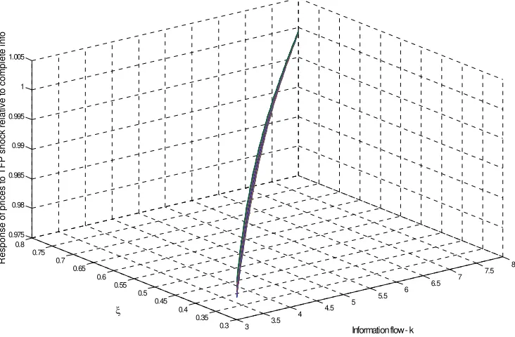
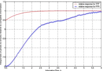
prices, ~is positive at 0:17. In F igure 2;I plot the price responses to the two shocks under
rational inattention as a fraction of the response under perfect information, and expressed as a function of . The closer the fraction is to 1, the closer the price responses under rational
inattention are to the ones under complete information. With low values of the …rm will
pay attention only to the technology shocks,"a
t;not responding at all to the monetary policy
shocks, "r
t. As increases, the response to the technology shocks converges quickly to the
complete information one, while the one to the monetary policy shocks has a much slower
convergence. In F igure 3; I plot the value of the attention multiplier, ; as a function of
. For small enough values of there is a corner solution in attention allocation. As
increases the attention multiplier converges, as expected, to 1; but remains substantially
large for intermediate values. In F igure 4; I plot the attention multiplier ; as a function
of ; setting equal to 3. For low values of ; and therefore for large degrees of strategic
complementarities in prices, theattention multiplier gets particularly large, pushing towards
a corner solution where all the attention is allocated to the technology shocks. In F igures
5 and 6; I plot the relative responses of prices to shocks to"a
t and "rt as a function of both
and : A larger increases the relative responses of prices to both shocks, while a larger
reduces strategic complementarities in prices, and everything else being equal, increases
price responses to both shocks. It has to be said that a value of equal to 6 is already
5
The numerical solution to the model
In this section I solve the dynamic model introduced in section 3 with numerical methods. In subsection 5.1, I describe the numerical routine, in subsection 5.2, I choose the parameters of the model and in subsection 5.,3 I comment the results of the attention allocation problems and the implied dynamics of aggregate prices.
5.1
The solution routine
I apply a two-step solution procedure28. In the …rst step I formulate a guess for the aggregate
price, P^t; a guess for the aggregate capital-to-labor ratio, k^t; and a guess for the aggregate
intermediate-inputs ratio, x^t; all in log-deviations from the non-stochastic balanced growth
path, and solve for the dynamics of the model economy.
In the second step, I solve for the optimal allocation of attention of each decision maker, given the processes for the endogenous variables of the model economy obtained in the …rst
step. In order to solve each agent’s attention allocation problem; I take a log-quadratic
expansion of the sum of the discounted expected pro…ts around the non-stochastic balanced
growth path29. In order to save on space, I express the attention allocation problems of the
three decision makers in terms of the variable^j;t(z); which I de…ne in the following way:
^
j;t(z)
8 > <
> :
^
Pt(z); j =p
^
kt(z); j =k
^
xt(z); j =x
:
The attention allocation problem for the decision maker choosing ^j;t(z) at …rm z, can be
28See Appendix B for more details.
29As discussed by Sims (2006) p. 161, and Ma´ckoviak and Wiederholt (2007) pp. 35-37, solving the
then expressed as:
min
fszj;tg2S!jE
^
j;t(z) ^
y
j;t(z)
2
(27)
s:t:
i) : ^j;t(z) = Eh^j;ty (z)jstzji; (28)
ii) : I
n
y
aj;t(z);
y
rj;t(z)
o
;fszj;tg j; (29)
iii) : ^yj;t(z) =
y
aj;t(z) +
y
rj;t(z) (30)
where !j > 0, ^
y
j;t(z) is the log-deviation from the non-stochastic balanced growth path of
the optimal choice of yj;t(z)in the case of a perfectly informed decision makerj; and ^j;t(z)
is the projection of ^yj;t(z) on the realization of signals for decision maker j; up to time t;
and at …rm z. The processes forn yaj;t(z); yrj;t(z)o are obtained from the …rst step. I can
then solve the attention allocation problems in (27) (30), obtaining the implied processes
for aggregate prices, capital-to-labor ratio and intermediate-inputs ratio:
^
Pt =
Z 1
0
^
Pt (z)dz;
^
kt =
Z 1
0
^
kt(z)dz;
^
xt =
Z 1
0
^
xt (z)dz:
I then update the guess and start again from the …rst step, iterating until convergence.
5.2
Calibration
I set the discount factor equal to 0:99. The depreciation rate is equal to 0:025: The
elasticity of value added output with respect to capital, , is assumed to be 0:36, a value
roughly consistent with observed income shares. I set the habit parameterbequal to0:7, and
the inverse of the Frisch’s elasticity, l;equal to1;similar to Altig, Christiano, Eichenbaum,
and Linde (2005). I choose 0so that on the non-stochastic balanced growth path households
supply an amount of labor equal to one. The dynamics of capital adjustment costs around the non-stochastic balanced growth path are shaped by the second derivative of the capital
adjustment cost function evaluated at steady state, S00(1):I set the capital adjustment cost
Eichenbaum, and Linde (2005), but it is slightly smaller than the one obtained by Smets and Wouters (2007). The elasticity of the cost of capital utilization, = 000(1)(1), is set to0:5;
which is similar to the value estimated by Burnside and Eichenbaum (1996). I choose the
elasticity of substitution across goods, ;and the share of intermediate inputs in total costs,
; following Nakamura and Steinsson (2007)30. Therefore, I set equal to 4; and equal
to 0:75: From input-output tables relative to the U.S. economy, Nakamura and Steinsson
(2007) estimate that the weighted average of the share of intermediate inputs in revenues is
approximately 56 percent. Then, given the average markup implied by , the steady state
share of intermediate inputs in total costs of production is 0:75.
The parameters in the Taylor rule, r; and y; are obtained by estimating the rule31
on the U.S. data from 1959:2 to 2007:2. I estimate the Taylor rule through an e¢cient GMM estimator similar to Clarida, Gali and Gertler (2000). The instruments set includes
the four lags ofrt; tandyt;and the four lags of in‡ation in commodity prices, of M2 growth
and of the ”spread” between the ten years and the three months U.S. treasury bonds32.
Table 3 contains the results of the estimation with associated robust standard errors in
parenthesis. Therefore, r; and y are set equal to 0:96;0:12 and 0:2 respectively. The
test of overidentifying restrictions rejects the null at one percent signi…cance level. The
autocorrelation coe¢cient, a;and the constant, a;are chosen according to the estimates of
an AR(1) process on an estimate of the U.S. quarterly growth rate in TFP33, from 1959:2 to
2007:2. The estimated autoregressive coe¢cient cannot be statistically distinguished from
zero, therefore I set a = 0: The standard deviations of the two shocks, a and r; are
obtained respectively from the standard deviation of the U.S. quarterly growth rate in TFP;
and from the standard deviation of the residual of the estimated Taylor rule, over the period
30”Berry et al. (1995) and Nevo (2001) …nd that markups vary a great deal across …rms. The value of
I choose implies a markup similar to the mean markup estimated by Berry et al. (1995) but slightly below the median markup found by Nevo (2001). Broda and Weinstein (2006) estimate elasticities of demand for a large array of disaggregated products using trade data. They report a median elasticity of demand below 3. Also, Burstein and Hellwig (2006) estimate an elasticity of demand near 5 using a menu cost model. Midrigan (2005) uses = 3 while Golosov and Lucas (2006) use = 7.”
31The equation I estimate is:
rt=c+ rrt 1+ t+ yyt+urt;
wherertis the Federal Fund rate, tis the log-di¤erence in the GDP price de‡ator, andytis the deviation
of the growth rate of output from a linear trend.
32Quarterly measures were computed averaging over months.
33Fernald (2007) estimates a quarterly series for the U.S. TFP growth rate trough a Solow residual
1959:2-2007:2: The standard deviation of the U.S. quarterly growth rate in TFP is about 4
times the standard deviation of the residual from the Taylor rule34. In mapping the estimated
standard deviation of the TFP growth rate to the standard deviation of the technology shock in the model, I have to adjust for the fact that the TFP growth rate has been estimated
according to a model with a value added production function with no intermediate inputs35.
Therefore, I need to scale the standard deviation of the estimated TFP growth rate by1 .
Since has been set equal to 0:75, the ratio of standard deviations of shocks in the model,
a
r;is set equal to1:Finally the total information processing capabilities at the …rm level, ;
is chosen so that in equilibrium the loss each …rm faces from not being completely informed
is a relatively small fraction of pro…ts. Hence I choose equal to 4:
5.3
Results
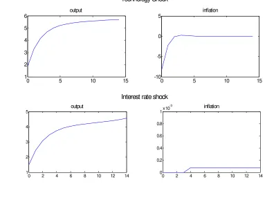
InF igure 7;I plot the responses of in‡ation and output to a one basis point shock to"a and
"r in the model under complete information, ! +1: Not surprisingly, almost all of the
adjustment in prices to "a takes place in two quarters, while all of the adjustment in prices
following the shock to "r takes place in the period of impact of the shock. Under complete
information, in fact, a one basis point positive shock to "a reduces prices by about12 basis
points on impact, and about 11 basis points after two quarters. A one basis point negative
shock to "r increases prices by approximately 8:5 basis points along with the shock. Since
the relative standard deviation of"a and "r is set equal to 1;and given that the impact of a technology shock on the complete information aggregate price level is larger than the impact
of an equally sized monetary policy shock, there is an initial incentive for the …rm to pay
more attention to technology shocks than to monetary policy shocks, but such an incentive is relatively small. Under complete information, in fact, the long-run impact of a one basis
point shock to"aon prices is about 30 percent larger than the long-run impact of a one basis
point shock to"r:Intuitively this initial incentive is the dynamic counterpart of the variable I derived in the static version of the model. Therefore, if this model has to generate a
large di¤erential in the response of prices to the two shocks, it must come from theattention
multiplier. Given that the monetary policy authority is substantially more aggressive on
output than it is on in‡ation, and that the share of intermediate inputs in total costs, ; is
34I obtain similar results if I use the standard deviations of the estimated TFP and monetary policy shocks
from the VAR.
0:75, the feedback from aggregate prices to …rm level complete information pro…t-maximizing price, P^ty(z); is substantial, inducing a large attention multiplier. In F igure 8; I plot the impulse responses of output and in‡ation in the model with limited information processing
capabilities, with equal to 4. Prices adjust quickly to the "a shock, with almost all of the
adjustment taking place in the …rst two quarters. In contrast, prices adjust very sluggishly to
the"rshock, inducing a large real e¤ect of the monetary policy shock. The response of output
to the"r shock is very persistent and takes many quarters to converge to zero. The optimal
allocation of across the di¤erent decision makers is such that 50 percent of is allocated to
price decision maker, 33 percent is allocated to the intermediate-inputs ratio decision maker and the remaining to the capital-to-labor ratio decision maker. The price decision maker allocates almost all of its information processing resources to the technology shocks. The other two decision makers allocate similar resources to the technology and monetary policy shocks, as the capital-to-labor ratio and the intermediate-inputs ratio have similar impacts across the two shocks on the variability of pro…ts. At equilibrium the marginal value of additional information processing resources at the …rm level is small. Each …rm faces a loss that is in the order of 1/1000 of its discounted sum of non-stochastic balanced growth path pro…ts, where the loss is computed relative to the case the …rm had complete information,
! 1; and everything else being equal.
6
Complementarities, monetary policy and signals
struc-ture
In this section I investigate the roles of strategic complementarity in price setting, monetary policy and the role of restrictions on the signals space for the results obtained above. Lastly, I discuss potential extensions and shortcomings.
6.1
The role of complementarities
I reduce the share of intermediate inputs in total steady state costs, ; from 0:75to 0:5. A
value of equal to0:75implied in section4a value of equal to0:5. With dropping to0:5;
increases to1; and the degree of strategic complementarity in price setting is substantially
the fact that Woodford (2003) recommends a value of between 0:15 and 0:1 in models of sticky prices.
With a smaller degree of strategic complementarity in price setting there are two e¤ects that reduce the di¤erence in the allocation of attention across the two shocks for the price setter. The …rst is a direct e¤ect that goes through the reallocation of attention at the price setter level: smaller complementarities in price setting induce smaller complementarities in the allocation of attention across price setters, and, everything else being equal, reduces the di¤erential in the allocation of attention across shocks for each price setter. The second e¤ect
relates to the reallocation of information processing resources, ; at the …rm level: smaller
complementarities in price setting induce a larger variability of aggregate prices in response to aggregate shocks, and, everything else being equal, increase the incentive to allocate more resources to process information about prices than to process information about the
capital-to-labor ratio and the intermediate-inputs ratio. At the equilibrium, 75 percent of total
information processing resources, ;is allocated to the price setter,16percent is allocated to
the intermediate-inputs ratio decision maker and the remaining to the capital-to-labor ratio
decision maker. The price setter allocates57percent of its attention to technology. Therefore
the di¤erential in attention allocation across the two shocks is substantially smaller for this decision maker relative to the case with larger complementairity in price setting. Capital-to-labor and intermediate-inputs ratios will not be very responsive to the monetary policy shocks, pushing the respective decision makers to allocate almost all of their attention to the
technology shocks. In F igure 9; I plot the responses of in‡ation to a one basis point shock
to "a and "r; in the model with and without limited information processing capabilities.
Now, the adjustment of prices to"r takes place in two quarters, and therefore, the real e¤ect
of the monetary policy shocks are small and in‡ation is not very persistent. Most of the
adjustment in prices to "a takes place in two quarters, similar to the benchmark calibration.
Since a
r is set equal to 2; the initial impact of a one basis point shock to "
a on pro…ts is
about 30 percent larger than theinitial impact of a one basis point shock to"r;and therefore
the price setter’s initial incentive to allocate more attention to technology is similar to the
benchmark calibration36. However, with low complementarities in price setting, the initial
incentive does not get ampli…ed and the di¤erence in the allocation of attention across the two shocks will be small.
36By the same argument in section5:2;lowering to0:5;causes the relative standard deviation of shocks, a
6.2
The role of monetary policy
In this paragraph I modify the parameterization of the monetary policy rule de…ned in (5):
First, I decrease y from0:2to0:1, making the monetary authority less aggressive on output
growth. A less aggressive monetary policy on output growth a¤ects the speed of adjustment of prices to the two aggregate shocks mainly through three channels. The …rst two channels have to do with the allocation of attention at the price-setter level, the third channel is related to the allocation of attention decision at the …rm level. A less aggressive monetary policy on output growth, reduces the variability of prices following technology shocks, therefore
reducing theinitial incentive to allocate attention to these shocks. The drop in y is so large
that the price setter has an initial incentive to allocate more attention to monetary policy
shocks, being prices relatively more volatile to those shocks than to technology shocks under
complete information. The second impact of the lower y is on the price setter’s allocation
of attention that takes place through a lowerattention multiplier: a less aggressive monetary
policy on output growth reduces the feedback from aggregate prices to …rms level complete information pro…t-maximizing prices, inducing lower complementarities in the allocation of attention. Finally there is a reallocation of information processing resources at the …rm level: more resource devoted to process information on the variability of prices to monetary policy shocks cause prices to be more responsive to such shocks, and, as a consequence, the capital-to-labor ratio and the intermediate-inputs ratio to have a smaller variability following monetary policy shocks, as the economy dynamics following these shocks are closer to the complete information counterparts. It follows that the price decision becomes relatively more important than the other two decisions. Therefore more information processing capabilities
are allocated to the price setter. In fact, 76percent of goes to the price setter,17percent
goes to the intermediate-inputs decision maker, and the residual goes to the capital-to-labor
ratio decision maker. The price setter allocates 58 percent of her information processing
capabilities to monetary policy shocks, and 42 percent to technology shocks. Unlike the
benchmark speci…cation, there is no substantial ampli…cation in the di¤erential allocation
of attention in favor of the monetary policy shocks. In F igure 10; I plot the responses of
in‡ation to a one basis point shock to "a and "r; in the model with and without limited
information processing capabilities. The speed of adjustment of prices to the two aggregate shocks is similar, with prices adjusting slightly more quickly to"r than to "a:
In the second modi…cation to the parameterization of the Taylor rule, I increase from
induces a more aggressive monetary policy on in‡ation, which reduces, everything else being equal, the variability of prices to any shock. The impact on the allocation of attention is similar to the impact caused by a decrease in the degree of strategic complementarity in price setting. The …rst direct e¤ect goes through the reallocation of attention at the price setter level: a more aggressive monetary policy on in‡ation reduces the feedback from aggregate prices to …rms level complete information pro…t-maximizing prices, inducing lower comple-mentarities in the allocation of attention, and therefore more attention devoted to monetary policy shocks relative to the benchmark parameterization. The second, indirect, e¤ect re-lates to the reallocation of information processing resources at the …rm level: when price setters allocate more resources to process information on the variability of prices following monetary policy shocks, aggregate prices become more responsive to such shocks, and, as a consequence, the capital-to-labor ratio and the intermediate-inputs ratio become less respon-sive to monetary policy shocks. It follows that the price setter is allocated more resources
relative to the benchmark parameterization. In contrast to the case in which I changed y;a
change in has no substantial impact on theinitial incentive for the price setter to allocate
more attention to technology shocks. As in the benchmark parameterization, there is an
ini-tial incentive to allocate more resources to process information about technology shocks, but
here there is no large ampli…cation of this incentive through theattention multiplier. At the
solution, the price setter allocates 56 percent of her information processing capabilities to
the technology shocks. Similarly to the case of a less aggressive monetary policy on output growth, the capital-to-labor and intermediate-inputs ratios will be not very responsive to the monetary policy shocks, and hence the respective decision makers will allocate almost
all of their attention to technology shocks. In equilibrium,64percent of is allocated to the
price setter. In F igure 11; aggregate prices have similar speeds of adjustments to the two
aggregate shocks.
The ability of the model to generate the di¤erential response in prices depends, then, on the fact that the monetary policy, estimated over the sample period 1959:2-2007:2, has been relative more aggressive on output growth than it has been on in‡ation. When I estimate
the same policy rule on the sub-sample37 from 1979:3, to 2007:2, I obtain that the monetary