Five Steps Block Predictor Block Corrector Method for the Solution of y'' = f (x,y,y')

http://dx.doi.org/10.4236/am.2014.58117

Five Steps Block Predictor-Block Corrector

Method for the Solution of

_y

′′

₌

_{f x y y}

(

_{, ,}

′

)

Mathew Remilekun Odekunle1, Michael Otokpa Egwurube1, Adetola Olaide Adesanya1,

Mfon Okon Udo2

1_{Department of Mathematics, Modibbo Adama University of Technology, Yola, Nigeria}

2_{Department of Mathematics and Statistics, Cross River University of Technology, Calabar, Nigeria}

Email: [email protected], [email protected]

Received 15 February 2014; revised 15 March 2014; accepted 22 March 2014

Copyright © 2014 by authors and Scientific Research Publishing Inc.

This work is licensed under the Creative Commons Attribution International License (CC BY). http://creativecommons.org/licenses/by/4.0/

Abstract

Theory has it that increasing the step length improves the accuracy of a method. In order to affirm this we increased the step length of the concept in [1] by one to get k = 5. The technique of colloca-tion and interpolacolloca-tion of the power series approximate solucolloca-tion at some selected grid points is considered so as to generate continuous linear multistep methods with constant step sizes. Two, three and four interpolation points are considered to generate the continuous predictor-corrector methods which are implemented in block method respectively. The proposed methods when tested on some numerical examples performed more efficiently than those of [1]. Interestingly the concept of self starting [2] and that of constant order are reaffirmed in our new methods.

Keywords

Step Length, Power Series, Block Predictor, Block Corrector, Constant Order, Step Size, Grid Points, Self Starting, Efficiency

1. Introduction

In this paper we examine the solution to general second order initial value problem of the form

(

, ,

) ( )

, 0 0,

( )

0 0

bur-densome since it no longer requires special ways to incorporate the subroutine to supply the starting values. As a result, this leads to computer time and human effort conservation.

The new methods are continuous in nature with the advantage of possible evaluation at all points within the integration interval. We have taken advantage of the works of [7] [12]-[15] who proposed direct block methods as predictor in the form

( ) ( ) 1 ( )

_{( )}

_{( )}

0 2

0

i i

m n i n i m

i

A Y ey h d f y b f y

=

 

=

∑

+ _ + _ (2)

where

[

]

T

1 2

m n n n n r

Y = y y₊ y₊  y₊

( )

[

]

T

1 2

m n n n n r

f y = f f ₊ f ₊  f ₊

( )

[

]

T

1 2 3

n n n n n

f y = f ₋ f ₋ f ₋  f

i

e = ×r r matrix, A( )0 = ×r r identity martix.

And also the discrete block formula as corrector in the form

( )0 ( ) ( ) 2 ( )0 ( )

1 2 1

i k i

m m m m m

A Y =A Y − +A Y − +h B f − +B f  (3)

where A( )0 = ×r r identity matrix

[

]

T

1 1 2 3

m n n n n

f ₋ = f ₋ f ₋ f ₋  f

[

]

T

1 1 2 3

m n n n n

Y ₋ = y₋ y₋ y₋  y

[

]

T

2 1 2 3

m n n n n n k

Y ₋ = y′₋ y′₋ y′₋  y′ y′₊

[

]

T

1 2

m n n n s

f = f ₊ f ₊  f ₊

with the aim to cater for some of the setbacks of predictor-corrector method [16] [17]. The fact that interpolation point cannot exceed the order of the differential equation for block methods is worrisome [9]. Also vital to this paper is the concept of block predictor-corrector method (Milne approach). This method formed a bridge be-tween the predictor-corrector method and block method [4] [10] [13]. In [1] we stated that results generated at an overlapping interval affect the accuracy of the method and the nature of the model cannot be determined at the selected grid points.

In this paper as in [1], we developed a method using the Milne approach but the corrector was implemented at a non overlapping interval. The numerical experiment compared the results generated at different step lengths, when k = 4 and when k = 5 respectively.

2. Methodology

2.1. Development of the Continuous Linear Multistep Methods

We consider a power series approximate solution in the form

( )

2

0 r s

j j j

y x a x

+ −

=

=

∑

(4)

where r and s are the number of interpolation and collocation points respectively. The second derivative of (4) gives

( )

2

(

)

2 2

1 r s

j j j

y x j j a x

+ −

−

=

′′ =

∑

− (5)

Substituting (5) into (1) gives

(

)

2

(

)

2 2

, , 1

r s

j j j

f x y y j j a x

+ −

−

=

Interpolating (4) and collocating (6) at some selected grid points gives a system of non linear equations in the form

AX =U (7)

where

[

]

T

0 1 2 3 r s1

A= a a a a  a_{+ −}

[

]

T

1 1

n n n r n n n s

U= y y₊  y₊ f f ₊  f ₊

(

)(

)

(

)(

)

(

)(

)

2 3 1

2 3 1

1 1 1 1

2 3 1

1 1

1 1

1 1

1

1

0 0 2 6 1 2

0 0 2 6 1 2

0 0 2 6 1 2

r s

n n n n

r s

n n n n

r s

n r n r n r n r

r s

n n

r s

n n

r s

n s n s

x x x x

x x x x

x x x x

X

x s r s r x

x s r s r x

x s r s r x

+ −

+ −

+ + + +

+ −

+ + + +

+ −

+ −

+ +

+ −

+ +

 

 

 

 

 

 

=  _{+ − + −} 

 

+ − + −

 

 

 

 + − + − 

 

 

      

 

      

Solving (7) for the unknown constants a s′j using Guassian elimination method and substituting back into (4) gives a continuous linear multistep method in the form

( )

( )

2

( )

0 0

r s

j n j j n j

j j

y t α t y+ h β t f+

= =

=

∑

+

∑

(8)

where α_j

( )

t and β_j

( )

t are polynomials,

(

) (

)

(

, ,

)

, n

n j n n n

x x

f fx jh y x jh y x jh t

h +

− ′

= + + + =

2.1.1. Development of the Block Predictor

Interpolating (4) at xn r+ ,r=0,1 and collocating (6) at xn s+ ,s=0 1 5.

( )

the parameters in (7) becomes

[

]

T

0 1 2 3 4 5 6 7

A= a a a a a a a a

[

]

T

1 1 2 3 4 5

n n n n n n n n

U= y y₊ f f ₊ f ₊ f ₊ f ₊ f ₊

2 3 4 5 6 7

2 3 4 5 6 7

1 1 1 1 1 1 1

2 3 4 5

2 3 4 5

1 1 1 1 1

2 3 4 5

2 2 2 2 2

2 3 4 5

3 3 3 3 3

4 1

1

0 0 2 6 12 20 30 42

0 0 2 6 12 20 30 42

0 0 2 6 12 20 30 42

0 0 2 6 12 20 30 42

0 0 2 6

n n n n n n n

n n n n n n n

n n n n n

n n n n n

n n n n n

n n n n n

n

x x x x x x x

x x x x x x x

x x x x x

x x x x x

X

x x x x x

x x x x x

x

+ + + + + + +

+ + + + +

+ + + + +

+ + + + +

+ =

2 3 4 5

4 4 4 4

2 3 4 5

5 5 5 5 5

12 20 30 42

0 0 2 6 12 20 30 42

n n n n

n n n n n

x x x x

x x x x x

+ + + +

+ + + + +

 

 

 

 

 

 

 

 

 

 

 

 

 

Solving for the unknown constants a s′_j using Guassian elimination method and substituting into (4), makes Equation (8) reduced to

( )

1

( )

5

( )

2

0 0

j n j j n j

j j

y t α t y+ h β t f+

= =

where

0 1 t α = −

1 t α =

(

7 6 5 4 3 2

)

0

1

2 42 357 1575 3836 5040 2462

10080 t t t t t t t

β = − − + − + − +

(

7 6 5 4 3

)

1

1

10 196 1491 5390 8400 4315

10080 t t t t t t

β = − + − + −

(

7 6 5 4 3

)

2

1

10 182 1239 3745 4200 1522

5040 t t t t t t

β = − − + − + −

(

7 6 5 4 3

)

3

1

10 168 1029 2730 2800 941

5040 t t t t t t

β = − + − + −

(

7 6 5 4 3

)

4

1

10 154 861 2135 2100 682

10080 t t t t t t

β = − − + − − −

(

7 6 5 4 3

)

5

1

2 28 147 350 336 107

10080 t t t t t t

β = − + − − −

Solving for the independent solution in (9) and simplifying gives

( )

( )

_{( )}

1 5

2 0 ! 0

i i

n j n j n j

i j

jh

y y h t f

i σ

+ +

= =

=

∑

+

∑

(10)

where

(

7 6 5 4 3 2

)

0

1

2 42 357 1575 3836 5040

10080 t t t t t t

σ = − − + − + −

(

7 6 5 4 3

)

1

1

10 196 1491 5390 8400

10080 t t t t t

σ = − + − +

(

7 6 5 4 3

)

2

1

10 182 1239 3745 4200

5040 t t t t t

σ = − − + − +

(

7 6 5 4 3

)

3

1

10 168 1029 2730 2800

5040 t t t t t

σ = − + − +

(

7 6 5 4 3

)

4

1

10 154 861 2135 2100

10080 t t t t t

σ = − − + − +

(

7 6 5 4 3

)

5

1

2 28 147 350 336

10080 t t t t t

σ = − + − −

Evaluating (10) at the selected grid points, the parameters in (2) gives the following I) When i=0

( )0

5 5

A = × identity matrix

( )0

_[

_]

T

1 2 3 4 5

m n n n n n

0

0 0 0 0 1 0 0 0 0 1 , 0 0 0 0 1 0 0 0 0 1 0 0 0 0 1 e

 

 

 

 

=

 

 

 

 

1

0 0 0 0 1 0 0 0 0 2 0 0 0 0 3 0 0 0 0 4 0 0 0 0 5 e

 

 

 

 

=

 

 

 

 

0

1231

0 0 0 0

5040 71

0 0 0 0

126 123

0 0 0 0

140 376

0 0 0 0

315 1525

0 0 0 0

1008

d

 

 

 

 

 

 

 

=

 

 

 

 

 

 

 

, 0

863 761 941 341 107

2016 2520 5040 5040 10080

544 37 136 101 8

315 63 315 630 315

3501 9 87 9 9

1120 140 112 35 224

1424 176 608 16 16

315 315 315 63 315

11875 625 3125 625 275

2016 504 1008 1008 2016

b

− −

 

 

 

− −

 

 

 _{− −} 

 

=

 

 ₋ 

 

 

 

 

 

II) When i=1

( )

[

]

T

1 2 3 4 5

i

m n n n n n

Y = y′+ y′+ y′+ y′+ y′+

1

0 0 0 0 1 0 0 0 0 1 0 0 0 0 1 0 0 0 0 1 0 0 0 0 1 e

 

 

 

 

=

 

 

 

 

, ₁

95

0 0 0 0

288 14

0 0 0 0

45 51

0 0 0 0

160 14

0 0 0 0

45 95

0 0 0 0

288

d

 

 

 

 

 

 

 

=

 

 

 

 

 

 

 

1

1427 133 241 173 3

1440 240 720 1440 160

43 7 7 1 1

30 45 45 15 90

219 57 57 21 3

160 80 80 160 160

64 8 64 14

0

45 15 45 45

125 125 125 125 95

96 144 144 96 288

b

− −

 

 

 

−

 

 

 ₋ 

 

=

 

 

 

 

 

 

 

2.1.2. Development of the Block Corrector

Here there are three cases (I, II and III) to be considered. Development of the Block Corrector for Case I

Interpolating (4) at x_{n r+} ,r=0 1 2

( )

and collocating (6) at x_{n s+} ,s=0 1 5,

( )

makes Equation (7) reduced to

[

]

T

0 1 2 3 4 5 6 7 8

[

]

T 1 2 3 1 2 3 4

n n n n n n n n n

U= y y₊ y₊ y₊ f f ₊ f ₊ f ₊ f ₊

2 3 4 5 6 7 8

2 3 4 5 6 7 8

1 1 1 1 1 1 1 1

2 3 4 5 6 7 8

2 2 2 2 2 2 2 2

2 3 4 5 6

2 3 4 5 6

1 1 1 1 1 1

2

2 2

1 1 1

0 0 2 6 12 20 30 42 56

0 0 2 6 12 20 30 42 56

0 0 2 6 12 20

n n n n n n n n

n n n n n n n n

n n n n n n n n

n n n n n n

n n n n n n

n n n

x x x x x x x x

x x x x x x x x

x x x x x x x x

x x x x x x

X x x x x x x

x x x

+ + + + + + + +

+ + + + + + + +

+ + + + + +

+ + +

=

3 4 5 6

2 2 2 2

2 3 4 5 6

3 3 3 3 3 3

2 3 4 5 6

4 4 4 4 4 4

2 3 4 5 6

5 5 5 5 5 5

30 42 56

0 0 2 6 12 20 30 42 56

0 0 2 6 12 20 30 42 56

0 0 2 6 12 20 30 42 56

n n n

n n n n n n

n n n n n n

n n n n n n

x x x

x x x x x x

x x x x x x

x x x x x x

+ + +

+ + + + + +

+ + + + + +

+ + + + + +

 

 

 

 

 

 

 

 

 

 

 

 

 

 

Solving for the unknown constants a s′j using Guassian elimination method and substituting into (4), makes Equation (8) reduced to

( )

2

( )

5

( )

2

0 0

j n j j n j

j j

y t α t y+ h β t f+

= =

=

∑

+

∑

(11)

where

(

8 7 6 5 4 3

)

0 1

3 60 476 1890 3836 3360 1437 442

442 t t t t t t t

α = − − + − + − + −

(

8 7 6 5 4 3

)

1 1

3 60 476 1890 3836 3360 1216

221 t t t t t t t

α = − + − + − +

(

8 7 6 5 4 3

)

2 1

3 60 476 1890 3836 3360 995

442 t t t t t t t

α = − − + − + − +

(

8 7 6 5 4 3 2

)

0

1

1134 23122 189210 793317 1798083 2117836 1113840 167922

2227680 t t t t t t t t

β = − + − + − + −

(

8 7 6 5 4 3

)

1

1

13167 261130 2045848 7965699 15645014 12890640 3413440

2227680 t t t t t t t

β = − + − + − +

(

8 7 6 5 4 3

)

2

1

126 4730 60214 353199 988757 1069320 378152

1113840 t t t t t t t

β = − + − + − +

(

8 7 6 5 4 3

)

3

1

441 6610 32844 50421 39438 124880 61696

1113840 t t t t t t t

β = − + − − + −

(

8 7 6 5 4 3

)

4

1

378 5350 25942 47859 11501 40740 25352

2227680 t t t t t t t

β = − − + − + + −

(

8 7 6 5 4 3

)

5

1

63 818 3808 7203 3206 3696 2752

2227680 t t t t t t t

β = − + − + + −

Evaluating (11) at t=3 1 5

( )

gives the following

(

)

3 1 2

2

1 2 3 4 5

31 159 411

221 221 221

337 11783 42998 5738 407 31

53040

n n n n

n n n n n n

y y y y

h

f f f f f f

+ + +

+ + + + +

= − − +

+ + + + − +

(12)

(

)

4 1 2

2

1 2 3 4 5

93 256 570

=

221 221 221

77 1864 5714 3424 269 8

3315

n n n n

n n n n n n

y y y y

h

f f f f f f

+ + +

+ + + + +

− − +

+ + + + + −

(

)

5 1 2

2

1 2 3 4 5

66 795 950

221 221 442

163 35 14206 10162 5653 347

5304

n n n n

n n n n n n

y y y y

h

f f f f f f

+ + +

+ + + + +

= − +

− − − − − −

(14)

Evaluating the first derivatives of (11) at t=0,1 gives the following

(

)

1 2

2

1 2 3 4 5

1437 1216 995

442 221 442

20999 426680 94538 15424 3169 344

278460

n n n n

n n n n n n

hy y y y

h

f f f f f f

+ +

+ + + + +

′ = − + −

− − − + − +

(15)

(

)

1 1 2

2

1 2 3 4 5

17 30 43

26 13 26

5035 114965 36658 6754 1459 163

131040

n n n n

n n n n n n

hy y y y

h

f f f f f f

+ + +

+ + + + +

′ = − +

− + + − + −

(16)

Writing Equations (12) to (16) in block form, the parameters in (3) gives the following

( )0

5 5

A = × identity matrix

[

]

T

1 2 3 4 5

m n n n n n

Y = y₊ y₊ y₊ y₊ y₊

[

]

T

1 1 2 3 4

m n n n n n

Y ₋ = y₋ y₋ y₋ y₋ y

[

]

T

2 1 2 3 1

m n n n n n

Y ₋ = y′₋ y′₋ y′₋ y′ y′₊

( )

[

]

T

1 2 3 4 5

m n n n n n

F Y = f ₊ f ₊ f ₊ f ₊ f ₊

( )

[

]

T

1 2 3 4

n n n n n n

F y = f ₋ f ₋ f ₋ f ₋ f

( )

0 0 0 0 1 0 0 0 0 1 0 0 0 0 1 0 0 0 0 1 0 0 0 0 1 i

A

 

 

 

 

=

 

 

 

 

, ( )

731 995

0 0 0

1726 1726 510 1216

0 0 0

863 863

1371 3807

0 0 0

1726 1726 892 2560

0 0 0

863 863

1755 6875

0 0 0

1726 1726 k

A

 

 

 

 

 

 

 

=

 

 

 

 

 

 

 

( )0

313679

0 0 0 0

5799360 10733

0 0 0 0

108738 291909

0 0 0 0

1933120 19496

0 0 0 0

90615 692425

0 0 0 0

3479616

B

 

 

 

 

 

 

 

=

 

 

 

 

 

 

 

( )

166091 152063 18133 9271 3373

1159872 8699040 2899680 5799360 17398080

17978 52613 10844 4873 278

54369 271845 271845 543690 271845

1817379 1119303 37209 3033 2277

1933120 966560 966560 386624 1933120

143264 598768

90615 271

i

B

− − −

− −

− =

84928 1856 1312

845 90615 18123 271845

6761375 5997875 3074125 3822625 214775 3479616 1739808 1739808 3479616 3479616

 

 

 

 

 

 

 

 

 

 − 

 

 

 

 

 

In a similar way the results for cases II and III are summarized as: Development of the Block Corrector for Case II

( )0

5 5

A = × identity matrix

[

]

T

1 2 3 4 5

m n n n n n

Y = y₊ y₊ y₊ y₊ y₊

[

]

T

1 1 2 3 4

m n n n n n

Y ₋ = y₋ y₋ y₋ y₋ y

[

]

T

2 1 2 3 1

m n n n n n

Y ₋ = y′₋ y′₋ y′₋ y′ y′₊

( )

[

]

T

1 2 3 4 5

m n n n n n

F Y = f ₊ f ₊ f ₊ f ₊ f ₊

( )

[

]

T

1 2 3 4

n n n n n n

F y = f ₋ f ₋ f ₋ f ₋ f

( )

0 0 0 0 1 0 0 0 0 1 0 0 0 0 1 0 0 0 0 1 0 0 0 0 1 i

A

 

 

 

 

=

 

 

 

 

, ( )

792431 31306 297137

0 0

2091360 65355 2091360

25706 63872 41132

0 0

65355 65355 65355

343461 33696 669627

0 0

697120 21785 697120

28492 108544 124384 0 0

65355 65355 65355

523235 58750 311875

0 0

418272 13071 418272

k

A

 

 

 

 

   =      

−

 

         

( )0

13846067

0 0 0 0

329389200

1865753

0 0 0 0

41173650

848073

0 0 0 0

12199600

1105448

0 0 0 0

20586825

3455275

0 0 0 0

13175568

B

 

 

 

 

 

 

 

=  

 

 

 

 

 

 

( )

329732329 38625017 2811953 420667 72343

1317556800 658778400 658778400 658778400 1317556800

2956022 2956487 138308 38999 1634

20586825 20586825 20586825 41173650 20586825

10555029 15699717 2674947

48798400 24399200 2

i

B

− − −

− − −

= 177633 24597

4399200 24399200 48798400

3023456 24355376 22196416 1491376 30752

205868825 20586825 20586825 20586825 20586825

132019375 101369375 45105625 29258125 3184175

52702272 26351136 26351136 26351136 52702272

     

−

−



     

 

 

 

 

 

 

 

 _

Development of Block Corrector case III

( )0

5 5

A = × identity matrix

[

]

T

1 2 3 4 5

m n n n n n

Y = y₊ y₊ y₊ y₊ y₊

[

]

T

1 1 2 3 4

m n n n n n

Y ₋ = y₋ y₋ y₋ y₋ y

[

]

T

2 1 2 3 1

m n n n n n

Y ₋ = y′₋ y′₋ y′₋ y′ y′₊

( )

[

]

T

1 2 3 4 5

m n n n n n

F Y = f ₊ f ₊ f ₊ f ₊ f ₊

( )

[

]

T

1 2 3 4

n n n n n n

F y = f ₋ f ₋ f ₋ f ₋ f

( )

0 0 0 0 1 0 0 0 0 1 0 0 0 0 1 0 0 0 0 1 0 0 0 0 1 i

A

 

 

 

 

=

 

 

 

 

, ( )

6841087 155083 384281 1841969

0

19120320 424896 2124480 19120320

12109 5465 22633 1441

0

33195 6639 33195 11065

261933 125145 840051 396771

0

708160 141632 708160 708160

147292 13072 59696 77776

0

298755 6639 33195 298755

148645 0

42 k

A =

−

− 1763125 933125 1034375

4896 424896 424896 141632

 

 

 

 

 

 

 

 

 

 

 

 

 − 

 

 

( )0

49345421

0 0 0 0

1338422400

400784

0 0 0 0

10456425

1956279

0 0 0 0

49571200

707488

0 0 0 0

10456425

6932075

0 0 0 0

53536896

B

 

 

 

 

 

 

 

=  

 

 

 

 

 − 

 

( )

17385799 2629933 2157571 239231 59681 53536896 13384224 66921120 267684480 1338422400

1021711 690083 89164 2351 1153

4182570 2091285 2091285 2091285 20912850

2150361 392499 254553 16173 9914240 2478560 2478560 991 i B − − − − − − − − − − − = 3699 4240 49571200

728072 3253232 492224 28568 12808

2091285 2091285 418257 418257 10456425

168194375 88398125 14134375 65661875 2830775 53536896 13384224 13384224 53536896 53536896

               −       ₋      _{− − −}     

3. Analysis of the Properties of the Methods

3.1. Order of the Methods

3.1.1 Order of the Block Predictor

When i=0, if we take a Taylor series expansion, we get

( )

( ) ( )

_{( )}

_{( )}

_{( )}

_{( )}

_{( )}

( )

( ) ( )

_{( )}

_{( )}

_{( )}

_{( )}

_{( )}

2 0 2 2 0 2 0 2 2 0 1231 ! 5040

863 761 941 341 107

1 2 3 4 5

! 2016 2520 5040 5040 10080

2 71

2

! 126

544 37 136 101 8

1 2 3 4 5

! 315 63 315 630 15

j j

n n n n

j

j

j j j j j

j n j

j j

n n n n

j

j

j j j j j

j n j

h

y y hy h y

j

h y j

h

y y hy h y

j h y j ∞ = + ∞ + = ∞ = + ∞ + = ′ ′′ − − −   − _ − + − + _   ′ ′′ − − −  − − + − + 

∑

∑

∑

∑

( )

( ) ( )

_{( )}

_{( )}

_{( )}

_{( )}

_{( )}

( )

( ) ( )

_{( )}

_{( )}

_{( )}

_{( )}

_{( )}

2 0 2 2 0 2 0 2 2 0 3 123 3 ! 140

3501 9 87 9 9

1 2 3 4 5

! 1120 140 112 35 224

4 376

4

! 315

1424 176 608 16 16

1 2 3 4 5

! 315 315 315 63 315

j j

n n n n

j

j

j j j j j

j n j

j j

n n n n

j

j

j j j j j

j n j

h

y y hy h y

j

h y j

h

y y hy h y

j h y j ∞ = + ∞ + = ∞ = + ∞ + =   _ ′ ′′ − − −   − _ − + − + _   ′ ′′ − − −   − _ + + − + _  

∑

∑

∑

∑

( )

( ) ( )

_{( )}

_{( )}

_{( )}

_{( )}

_{( )}

2 0 2 2 0 0 5 1525 5 ! 1008

11875 625 3125 625 275

1 2 3 4 5

! 2016 504 1008 1008 2016

j j

n n n n

j

j

j j j j j

j n j

h

y y hy h y

j h y j ∞ = + ∞ + =                                 =                        _{− − ′− ′′}       ₋  _{+ + + +}    _ _   

∑

∑

Collecting coefficients in powers of h, we see that the order of the method is six and the error constant is

T

199 19 141 8 1375

24192 945 4480 189 24192

− − − − −

 

 

 

Also when i=1

T

863 37 29 8 275

60480 3780 2240 945 12096

− − − − −

 

 

 

3.1.2. Order of the Block Corrector for Case I

Taking a Taylor series expansion gives

( )

( ) ( )

_{( )}

( )

_{( )}

_{( )}

_{( )}

_{( )}

_{( )}

( )

( ) 1 2 0 0 2 2 0 0

731 995 313679

1

! 1726 1726 5799360

166091 152063 18133 9271 3373

1 2 3 4 5

! 1159872 8699040 2899680 5799360 17398080

2 510 1216

! 863 86

j

j

j j

n n n n n

j j

j

j j j j j

j n j

j j

n n n

j h

y y hy y h y

j

h y j

h

y y hy

j ∞ ∞ − = = + ∞ + = ∞ = ′ ′′ − − − − −   − _ + − + − _   ′ − − −

∑

∑

∑

∑

( )

_{( )}

( )

_{( )}

_{( )}

_{( )}

_{( )}

_{( )}

( )

( ) ( )

_{( )}

1 2 0 2 2 0 1 2 0 0 2 10733 1 3 108738

17978 52613 10844 4873 278

1 2 3 4 5

! 54369 271845 271845 543690 271845

3 1371 3807 291909

1

! 1726 1726 1933120

! j j n n j j

j j j j j

j n j j j j j

n n n n n

j j

j j n

y h y

h y j

h

y y hy y h y

j h y j ∞ − = + ∞ + = ∞ ∞ − = = + + ′′ −   − _ + − + − _   ′ ′′ − − − − −

∑

∑

∑

∑

( )

_{( )}

_{( )}

_{( )}

_{( )}

_{( )}

( )

( ) ( )

_{( )}

( )

_{( )}

_{( )}

2 0 1 2 0 0 2 2 0

1817379 1119303 37209 3033 2277

1 2 3 4 5

1933120 966560 966560 386624 1933120

4 892 2560 19496

1

! 863 863 90615

143264 598768 84928

1 2

! 90615 271845

j j j j j

j

j

j

j j

n n n n n

j j j j j j n j h

y y hy y h y

j h y j ∞ = ∞ ∞ − = = + ∞ + =  _{+ + + −}      ′ ′′ − − − − − + +

∑

∑

∑

∑

( )

( )

( )

( )

( ) ( )

_{( )}

( )

_{( )}

_{( )}

_{( )}

_{( )}

1 2 0 0 2 2 0 1856 1312

3 4 5

90615 18123 271845

5 1755 6875 692425

1

! 1726 1726 3479616

6761375 5997875 3074125 3822625 214775

1 2 3 4

! 3479616 1739808 1739808 3479616 3

j j j

j

j

j j

n n n n n

j j

j

j j j j

j n j

h

y y hy y h y

j h y j ∞ ∞ − = = + ∞ + =  _{+ −}      ′ ′′ − − − − − + + + +

∑

∑

∑

( )

0 5 479616 j                                 =                                  _ _   

and the order of our method is seven with error constant as

T

297137 1469 3543 15548 62375

3131654400 3495150 5523200 12233025 125266176

 ₋ 

 

 

In a similar way, we compute and summarize the order for cases II and III as follows.

3.1.3. Order of the Block Corrector for Case II

In this case the order of our method is eight with error constant as

T

1841969 1441 132257 9722 41375

158106816000 9149700 195193600 308802375 46846464

_{− − − −} 

 

 

3.1.4. Order of the Block Corrector for Case III

Also using the same approach, the order of our method is nine with error constant as

T

13573207 251351 80077 135967 8474525

5300152704000 82814886000 21811328000 5175930375 42401221632

−

 

 

 

3.2. Consistency of the Method

From the above, it clearly shows that our methods are consistent.

3.3. Zero Stability

A block method is said to be zero stable if h→0, the root r j_j; =1 1

( )

k of the first characteristics polynomials

( )

R 0,

ρ = that is ρ

( )

R =det_

∑

A R( )0 k−1_=0 satisfying R ≤1 must have multiplicity equal to unity [9]. Applying this rule, we have that

( )

1 0 0 0 0 0 0 0 0 1 0 1 0 0 0 0 0 0 0 1

0 0 0 1 0 0 0 0 0 0 1 0 0 0 1 0 0 0 0 0 1 0 0 0 0 1 0 0 0 0 1 r

ρ

   

   

   

   

= − =

   

   

   

   

where R=0, 0, 0, 0,1 for each method. Hence the methods are zero stable

4. Numerical Experiment

4.1. Implementation

We implement the proposed methods to verify their efficacies over existing methods. To be considered are, two cases for k = 4 [1] and three cases for k = 5. Four examples were considered at h = 0.01 and h = 0.05. All com-putations were made with the usage of MATLAB (R2010a). An error (Err) is defined in this paper as the abso-lute value of the difference between the computed and expected values. The following keys are used in display-ing our results on the tables for clearity.

CASE 1: Two interpolation points. CASE II: Three interpolation points. CASE III: Four interpolation points.

4.1.1. Test Problem I

Consider the non-linear ODE

( )

2

( )

( )

1

0, 0 1, 0 , 0.05 2

y′′−x y′ = y = y′ = h=

Exact Solution:

( )

1 1ln 2

2 2

x y x

x +   = + _{ }

−  

4.1.2. Test Problem 2

Consider the non-linear initial value problem

( )

2

2 2

y

y y

y

′

′′ = − ; π 1, π 3, 0.05.

6 4 6 2

y _{ }= y′ _{ }= h=

   

Exact solution: y x

( )

=

(

sin

( )

x

)

2.

4.1.3. Test Problem 3

Consider the initial value ODE

3

ex

y′′ = +y x ;

( )

0 3,

( )

0 5 , 0.01.

32 32

y = − y′ = − h=

Exact solution:

( )

4 ₃3

32e x

4.1.4. Test Problem 4

Consider the initial value problem

4

y′′ = − y; y

( )

0 =1,y′

( )

0 =2,h=0.01.

Exact solution: y x

( )

=cos 2x+sin 2x.

5. Discussion

[image:13.595.89.541.272.484.2] [image:13.595.87.541.510.720.2]

We have considered two non-linear and two linear second order initial value problems in this paper as shown in

Table 1 toTable 4. In [1] we compared our method with the existing methods like the block and block predic-tor-corrector and the results re-affirms the claim of [10] that though block predictor-corrector method takes longer time to implement, it gives better approximation than the block method. In this paper we extended the step length considered in [1] and considered varying the number of interpolation points to observe the effect on the performance of the method.

Table 1. Comparing results for different interpolation points.

Err for k = 4 Err for k = 5

Case I Case II Case I Case II Case III

0.1 1.148666e−10 1.117957e−10 6.959988e−12 6.973755e−12 6.980638e−12

0.2 2.304048e−10 2.361691e−10 1.471068e−11 1.468337e−11 1.470468e−11

0.3 4.070080e−10 4.174734e−10 2.956990e−11 2.969025e−11 2.974887e−11

0.4 5.871796e−10 5.994316e−10 6.953504e−11 7.023626e−11 7.063172e−11

0.5 9.923316e−10 9.767278e−10 1.086504e−11 1.177911e−10 1.174840e−10

0.6 1.414456e−09 1.357228e−09 2.316121e−10 2.327660e−10 2.347267e−10

0.7 2.664834e−09 2.329491e−09 3.954923e−10 3.931862e−10 3.991147e−10

0.8 4.005613e−09 3.317707e−09 5.231535e−10 5.297960e−10 5.332230e−10

0.9 8.804608e−09 6.384651e−09 1.076466e−09 1.115101e−09 1.138269e−09

1.0 1.414628e−08 9.537446e−09 1.379378e−09 1.882982e−09 1.864998e−09

Table 2. Comparing results for different interpolation points.

Err for k = 4 Err for k = 5

Case I Case II Case I Case II Case III

1.023 5.483646e−08 1.001313e−09 1.450115e−08 1.450198e−08 1.448318e−08

1.123 7.475030e−08 1.039073e−09 2.041163e−08 2.040973e−08 2.040707e−08

1.223 9.301246e−08 4.935578e−09 2.645463e−08 2.644890e−08 2.645422e−08

1.323 1.104840e−07 9.038723e−09 3.120210e−08 3.120180e−08 3.120062e−08

1.423 1.267508e−07 1.454907e−08 3.532345e−08 3.532144e−08 3.531459e−08

1.523 1.408839e−07 1.992274e−08 3.884826e−08 3.884982e−08 3.876058e−08

1.623 1.537364e−07 2.583176e−08 4.128344e−08 4.128357e−08 4.128494e−08

1.723 1.633737e−07 3.115442e−08 4.305053e−08 4.305124e−08 4.304851e−08

1.823 1.693086e−07 3.594488e−08 4.550337e−08 4.550378e−08 4.550700e−08

[image:14.595.88.541.101.305.2]

Table 3. Comparing results for different interpolation points.

Err for k = 4 Err for k = 5

Case I Case II Case I Case II Case III

0.1 6.486478e−13 6.483702e−12 4.023171e−14 4.025946e−14 4.024558e−14

0.2 1.532774e−12 1.530470e−12 1.813549e−13 1.813272e−13 1.813272e−13

0.3 2.785883e−12 2.778555e−12 4.665435e−13 4.665712e−13 4.665757e−13

0.4 4.523689e−12 4.509226e−12 9.578172e−13 9.578172e−13 7.577894e−13

0.5 7.014500e−12 6.983969e−12 7.742495e−12 7.742495e−12 1.742412e−12

0.6 1.048768e−11 1.043124e−11 2.944242e−12 2.944242e−12 2.944187e−12

0.7 1.546147e−11 1.536465e−11 4.737225e−12 4.737225e−12 4.737134e−12

0.8 2.238659e−11 2.222950e−11 7.365913e−12 7.365913e−12 7.365761e−12

0.9 3.227908e−11 3.202710e−11 1.117295e−11 1.117295e−11 1.117278e−11

1.0 4.601608e−11 4.561729e−11 1.663791e−11 1.663791e−11 1.663769e−11

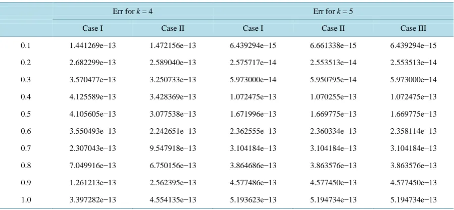
Table 4. Comparing results for different interpolation points.

Err for k = 4 Err for k = 5

Case I Case II Case I Case II Case III

0.1 1.441269e−13 1.472156e−13 6.439294e−15 6.661338e−15 6.439294e−15

0.2 2.682299e−13 2.589040e−13 2.575717e−14 2.553513e−14 2.553513e−14

0.3 3.570477e−13 3.250733e−13 5.973000e−14 5.950795e−14 5.973000e−14

0.4 4.125589e−13 3.428369e−13 1.072475e−13 1.070255e−13 1.072475e−13

0.5 4.105605e−13 3.077538e−13 1.671996e−13 1.669775e−13 1.669775e−13

0.6 3.550493e−13 2.242651e−13 2.362555e−13 2.360334e−13 2.358114e−13

0.7 2.307043e−13 9.547918e−13 3.104184e−13 3.104184e−13 3.104184e−13

0.8 7.049916e−13 6.750156e−13 3.864686e−13 3.863576e−13 3.863576e−13

0.9 1.261213e−13 2.562395e−13 4.577486e−13 4.577450e−13 4.577450e−13

1.0 3.397282e−13 4.554135e−13 5.193623e−13 5.194734e−13 5.194734e−13

6. Conclusion/Recommendation

In this paper we have proposed the varying of the step length from k = 4 [1] to k = 5. Block methods which have the properties of evaluation at all points within the interval of integration are adopted to give independent solu-tions at non overlapping intervals as predictors to the correctors. The new method k = 5 performed better than that of k = 4. Thus it has been confirmed that varying the step length improves the accuracy of the method. However, increasing the number of interpolation points does not significantly improve the result. We therefore, recommend the block predictor-block corrector method for use in the quest for solutions to second order initial value problems of ordinary differential equations.

References

[image:14.595.89.539.332.540.2]

Initial Value Problems. International Journal of Computer Mathematics, 86, 817-836. http://dx.doi.org/10.1080/00207160701708250

[3] Adesanya, A.O., Odekunle, M.R. and Adeyeye, A.O. (2012) Continuous Block Hybrid-Predictor-Corrector Method for the Solution of y′′= f x y y

(

, , ′

)

. International Journal of Mathematics and Soft computing, 2, 35-42.

[4] Adesanya, A.O., Odekunle, M.R. and Udo, M.O. (2013) Four Steps Continuous Method for the Solution of

(

, ,

)

.

y′′= f x y y′ American Journal of Computational Mathematics, 3, 169-174.

[5] Awoyemi, D.O. and Kayode, S.J. (2005) A Maximal Order Collocation Method for Direct Solution of Initial Value Problems of General Second Order Ordinary Differential Equation. Proceedings of the Conference Organised by the National Mathematical Centre, Abuja.

[6] Jator, S.N. (2007) A Sixth Order Linear Multistep Method for Direct Solution of y′=f x y y

(

, , ′

)

. International Jour- nal of Pure and Applied Mathematics, 40, 457-472.

[7] Awoyemi, D.O. (2001) A New Sixth Order Algorithm for General Second Order Ordinary Differential Equation. In-ternational Journal of Computer Mathematics, 77, 117-124.

[8] Awoyemi, D.O., Adebile, E.A., Adesanya, A.O. and Anake, T.A. (2011) Modifid Block Method for the Direct Solution of Second Order Ordinary Differential Equation. International Journal of Applied Mathematics and Computation, 3, 181-188.

[9] Lambert, J.D. (1973) Computational Methods in ODES. John Wiley and Sons, New York.

[10] Adesanya, A.O., Anake, T.A. and Udo, M.O. (2008) Improved Continuous Method for Direct Solution of General Second Order Ordinary Differential Equation. Journal of the Nigerian Association of Mathematical Physics, 13, 59-62.

[11] Udo, M.O., Olayi, G.A. and Ademiluyi, R.A. (2007) Linear Multistep Method for Solution of Second Order Initial Value Problems of Ordinary Differential Equations: A Truncation Error Approach. Global Journal of Mathematical Sciences, 6, 119-126.

[12] Zarina, B.I., Mohamed, S. and Iskanla, I.O. (2009) Direct Block Backward Differentiation Formulas for Solving Second Order Ordinary Differential Equation. Journal of Mathematics and Computation Sciences, 3, 120-122.

[13] James, A.A., Adesanya, A.O. and Sunday, J. (2013) Continuous Block Method for the Solution of Second Order Initial Value Problems of Ordinary Differential Equations. Journal of Mathematics and Computation Sciences, 83, 405-416.

[14] Awoyemi, D.O. and Idowu, M.O. (2005) A Class of Hybrid Collocation Method for Third Order Ordinary Differential Equation. International Journal of Computer Mathematics, 82, 1287-1293.

http://dx.doi.org/10.1080/00207160500112902

[15] Awoyemi, D.O., Udo, M.O. and Adesanya, A.O. (2006) Non-Symmetric Collocation Method for Direct Solution of General Second Order Initial Value Problems of Ordinary Differential Equations. Journal of Natural and Applied Sciences, 7, 31-37.

[16] Awoyemi, D.O. (2003) A p-Stable Linear Multistep Method for Solving Third Order Ordinary Differential Equation.

International Journal of Computer Mathematics, 80, 85-99. http://dx.doi.org/10.1080/0020716031000079572