Mathematical Analysis of a Large Scale Vector SIS Malaria Model in a Patchy Environment

http://dx.doi.org/10.4236/am.2014.513185

How to cite this paper: Wairimu,J., Gauthier, S. and Ogana, W. (2014) Mathematical Analysis of a Large Scale Vector SIS Malaria Model in a Patchy Environment. Applied Mathematics, 5, 1913-1926. http://dx.doi.org/10.4236/am.2014.513185

Mathematical Analysis of a Large Scale

Vector SIS Malaria Model in a Patchy

Environment

Josephine Wairimu1,2*, Sallet Gauthier2, Wandera Ogana1

1_{School of Mathematics, University of Nairobi, Nairobi, Kenya} 2_{INRIA, Metz and University of Lorraine, Lorraine, France}

Email: [email protected]

Received 20 April 2014; revised 26 May 2014; accepted 3 June 2014

Copyright © 2014 by authors and Scientific Research Publishing Inc.

This work is licensed under the Creative Commons Attribution International License (CC BY). http://creativecommons.org/licenses/by/4.0/

Abstract

We answer the stability question of the large scale SIS model describing transmission of highland malaria in Western Kenya in a patchy environment, formulated in [1]. There are two equilibrium states and their stability depends on the basic reproduction number, 0 [2]. If 0≤1, the

dis-ease-free steady solution is globally asymptotically stable and the disease always dies out. If

0 1

 > , there exists a unique endemic equilibrium which is globally stable and the disease persists. Application is done on data from Western Kenya. The age structure reduces the level of infection and the populations settle to the equilibrium faster than in the model without age structure.

Keywords

Highland Malaria, Differentiated Susceptibility and Infectivity, Monotone Dynamical Systems

1. Introduction

We recall the large scale system developed in [1] reduced into a compact form as

(

)

(

)

diag 1

X = −X X+ − +  X (1) where

(

, ,

)

X = x y z , is a vector representing; x is the proportion of infectious children, y is the proportion of infectious adults, and z is the proportion of infectious mosquitoes.

,  and the matrix  are the matrices.

( )

( )

( )

( )

( )

( )

( )

1 1 1 1 1

diag diag diag 0 0

0 diag diag diag 0

0 0 diag

C A N V N V N β β − − −       =         

( ) ( )

2

( ) ( )

2

0 0

0 0

diag diag diag diag 0

n

n

C C A A

I I N N β β       =       

(

)

(

)

( )

diag .1 0 0

diag 0

0 0 diag

C C h A A n h v I

γ ν µ

ν γ µ

µ  _{+ +}      = − +        0 0 0 0 0 0 C A v M M M     =           

The authors used the preceding matrices and the vector X =

(

x y z, ,

)

to rewrite Equation (10) in [1] in a compact form as

(

)

(

)

diag 1 .

X′ = −X X + − +  X (2) This system evolves on the unit cube of 3n.

Calculation of the Basic Reproduction Number

We use the classical framework defined in [3] [4].

The application 

( )

x =diag 1

(

−X

)

X represents the rate of appearance of new infections in the com- partments in the patches.

The function 

( )

X = − +

(

 

)

X is the rate of transfer of individuals in compartments.

If 

( )

x is set to zero, system becomes X = − +

(

 

)

X , which is a linear system, and we have already seen that

(

− + 

)

is a stable Metzler matrix.

Proposition 1.1

The basic reproduction number of system (1) is

(

)

(

1

)

0 ρ .

− = − − + 

   

Proof

This is straightforward since the Jacobian of  computed at the DFE X =0 is ,

F=

and the Jacobian of 

( )

X computed at the DFE is V= − +

(

 

)

.

The next generation matrix is then K= − − +

(

  

)

−1 □ We can develop the expression of 0 further:

( )

( )

( )

( )

( )

( )

( )

( ) ( )

( )

( ) ( )

1 1 1 1 2 2

0 0 diag diag diag

0 0 diag diag diag

diag diag diag diag diag diag 0

C

A

C C A A

v v

N V

F N V

N N

β

β

µ β µ β

− −       = _{=  }      

(

)

(

)

(

)

( )

diag 1 0 0

diag 0

0 0 diag

C C h A A n h v v M I M M γ ν µ

ν γ µ

µ − + + +      = − + =_ − + + _  _{− +}         

V (4)

Then we can compute the nonnegative matrix −V−1, which is a lower triangular matrix 11 1 21 22 33 0 0 0 0 0 V V V V − − − − −     − _{=  }     V with

(

)

(

)

(

)

(

)

(

(

)

)

(

)

(

)

( )

(

)

1 11 1 1 21 1 22 1 33 diag .1

diag diag .1

diag

diag

C C

h

A A C C

h h A A h v v V M

V M M

V M

V M

γ ν µ

ν γ µ γ ν µ

γ µ µ − − − − − − − − − = − − + + + = − + + − + + + = − − + + = − − +     

The next generation matrix is a block matrix

13 23

31 32

0 0

0 0 ,

0 K K K K K     =       with

( )

( )

( )

(

( )

)

( )

( )

( )

(

( )

)

( )

( ) ( )

(

(

)

)

( )

( ) ( )

(

(

)

)

(

(

)

)

( )

1 1 13 1 1 1 23 1 1 31 2 1 1 2 32

diag diag diag diag

diag diag diag diag

diag diag diag diag .1

diag diag diag diag diag .1

diag diag

C v

v

A v

v

C C C C

v h

A A A A C C

v h h

v

K N V M

K N V M

K N M

N M M

K

β µ

β µ

µ β γ ν µ

ν µ β γ µ γ ν µ

µ β − − − − − − − = − − + = − − + = − − + + + + − + + − + + + = −     

( ) ( )

(

(

)

)

1

2 diag diag

A A A A

h

N γ µ M

−

− + + 

The block structure of K implies (see [4]) that

(

)

2

0 =ρ K K31 13+K K32 23 

When 0<1, the DFE is locally asymptotically stable, and if 0 >1 the DFE is unstable, see [3] [4].

2. Main Result

In this section we establish a global stability result for the DFE when 0≤1 and a global stability result when 0>1

 . We have the following theorem Theorem 2.1

We consider the system (1) with the matrix MC+MA+Mv irreducible. Then

If 0≤1, then the system (1) is globally asymptotically stable at the origin If 0>1, then there exists a unique endemic equilibrium

*

X , which is globally asymptotically stable on

[ ]

3

0,1 n. ∈

K

We recall system (1),

(

)

diag 1

X = −X X+ − +_  _X

The Jacobian at the origin will be given by

( )

diag 1

(

)

diag

( )

J X = −X  − X + − +_  _

and

( )

0 .

J =+ − +_  _

To prove the first part of the proposition above we assume that 0≤1 Following [5], A= +B C is a re- gular splitting of A if B is Metzler stable and C≥0. Thus in our case _− + _ has to be a stable Metzler matrix which is invertible and ≥0, or equivalently, _− + _ has to be an M-matrix.

We know from Thieme [6], Driessche [4], and Varga [7] that

(

1

)

0 1 s 0.

−

 

≤ ⇔ − + − +_ _ ≤

   

From the preceding section we know that the Jacobian J is an irreducible Metzler matrix. So, by Perron- Frobenius, there exists a positive vector c0, such that

(

  − + 

)

Tc=s J

(

( )

0

)

c≤0. To prove the global stability of the DFE we consider the Lyapunov function

( )

,

L X = c X

where | , denotes the inner product. From the definition of c0, this function is actually positive definite in the nonnegative orthant.

We compute the derivative of L along the trajectories of (1) and find that it is equivalent to

( )

(

)

(

)

(

)

(

( )

)

(

( )

)

diag 1

T 0 0 0,

L X X X X

X s J X s J X

   

′ = − + − +_{ } ≤ + − +_{ }

 

= + − +_{ } = = ≤

c c

c c c

 



      

   (5)

We see that 0≤ X ≤1, it is clear that

(

1−X B

)

≤XB, hence the above inequality. Since s J

(

( )

0

)

≤0 the derivative is non positive. The DFE is stable.

We will prove the asymptotic stability when 0≤1.

First we consider the case when 0<1. Since we know that 0<1 implies s J

( )

<0, L′ is negative de- finite, since c0. This proves the asymptotic stability of the DFE.

When 0=1, we consider the largest invariant set contained in the set

( )

{

X L X′ 0 .

}

= =



For such an X we have

(

)

(

)

( )

0= cdiag 1−X X+ − +_  _X = c + − +_  _ X−diag X X , but since L x′

( )

=0, we have by the inequality (5),

(

+ − +_ _

)

X =0.

c   

Hence

( )

diag

( )

.

V′ X = − c X X

( )

( )

( )

( )

(

( ) ( )

2

( ) ( )

2

)

diag

diag diag

diag diag C diag C diag A diag A

x z

X X y z

z β N x β N y

      =    +    

We must have, for any index i, x zi i =0 and y zi i =0 Suppose xi=0 since

(

)

(

)

1 , 1, 1, 1 C n n j

C i C C C C

i i i i i h i i ij C j i ji

j j i j j i

i i

N V

x z x x m x x m

N N

β γ µ ν

= ≠ = ≠ ′ = − − + + +

∑

−

∑

we have 1 1, 0. C n j

C i C

i i i ij C j

j j i

i i

N V

x z m x

N N

β

= ≠

′ = +

∑

=

Then zi=0 and xj =0 for any patch j, with a “children” arc leaving j and entering i. Since zi =0 and xi=0 and since

(

)

(

)

2 2 ,

1, 1,

1 1

C A n n

j

C i A i v v

i i i i i i i v i i ij j i ji

j j i j j i

i i i

V

N N

z x z y z z m z z m

N N V

β β µ

= ≠ = ≠ ′ = − + − − +

∑

−

∑

we have 2 1, 0 A n j

A i v

i i i ij j

j j i

i i

V N

z y m z

N V

β

= ≠

′ = +

∑

=

Again yi=0 and zj =0 for any patch j with a “mosquito” arc leaving j and entering i. Now xi=yi=zi=0 implies

1,

A n

j

i ij A j

j j i i N

y m y

N = ≠

′ =

_∑

which implies that yj =0 for any patch with a “adult” arc leaving j and entering i.

Now, since any patch can be reached by a path composed of “children”, “adult” or “mosquito” arcs, this proves that xi= yi=zi =0 for any index.

This ends the proof for the global asymptotic stability of the DFE from LaSalle’s Invariance Principle [8]. To prove the second part of our theorem, when 0>1, we need the following theorem from [9]. Theorem 2.2

Let F be a 1

C vector field in _n

, whose flow φ preserves n₊ for t≥0 and is strongly monotone in n

+

 . Assume that the origin is an equilibrium and that all trajectories in n₊ are bounded. Suppose the matrix- valued map _DF: n n n

+ → +× +

   is strictly anti monotone, in the sense that,

( )

( )

if x< y, then DF x >DF y , then either all the trajectories in n \ 0

{ }

+

 tend to the origin, or else there is a unique equilibrium

(

)

n 0

p∈Int₊ p and all the trajectories in n₊ tend to p.

For our case we shall consider the positively invariant set

[ ]

0,13n, which is diffeomorphic to the nonnegative orthant 3₊n. Since the faces of the cube of type xi=1 are repulsive for the vector field associated to (1), all the trajectories are bounded in

[ ]

0,13n.

We recall system 1.

(

)

(

)

diag 1

X′ = −X X+ − +  X

If we take X1< X2∈X, then

( )

(

)(

)

( )

(

)(

)

1 1 1 1

2 2 2 2

diag 1

diag 1

F X X X X

F X X X X

Clearly

1 2,

X X

− +  < − +        since the quantities are positive.

Now we prove that

(

1

)(

1

)

(

2

)(

2

)

diag 1−X X < diag 1−X X

   

and hence show that the system is strongly monotone. That is

(

1

)

( )

1 1

( )

2

( )

2 2

diag X − diag X X < diag X − diag X X

      

or

( )

1 1

( )

2 2

diag X X diag X X .

−  < − 

Considering the structure of  and  and having X1<X2 in

[ ]

3

0,1 n and the fact that a sign change re- verses the inequality, then

( )

1 1

( )

2 2

diag X X > diag X X

   

hence

( )

1 1

( )

2 2

diag X X diag X X .

−_{ } < −_{ }

To prove that theorem, we recall the Jacobian J X

( )

of system (1)

( )

(

)

( ) diag diag 1 ,

J X = − X + −X + − +_  _

Again for any X1 <X2∈X , then diag 1

(

−X2

)

<diag 1

(

−X1

)

. Since the matrix  has on each row a

positive term, since  is a diagonal matrix with positive terms, we deduce

(

2

)

(

1

)

diag 1−X < diag 1−X

   

Considering the structure of  we have, if X1< X2, the relation X1<X2 holds and consequently

(

2

)

(

1

)

diag X diag X

−  < −  .

Finally we have J X

( )

2 <J X

( )

1 , therefore the anti monotone criteria is met. We will prove that no trajectory tends to the origin.

We have 0>1 which is equivalent to s J

(

( )

0

)

>1. Then there exists a positive vector c0 such that

( )

0T

(

)

T

(

( )

0

)

.

J c=   − +  c=s J c We consider the Chetaev function on a neighborhood of the origin

( )

.

V X = c X

An simple computation gives

( )

(

( )

)

_n diag

( )

.

V′ X = c_s J o I − X _X

Then in a sufficiently small neighborhood of the origin, in

[ ]

0,13n, V′

( )

X >0. This proves that for ε >0 sufficiently small, the hyperplane

{

X c X =ε

}

is a barrier for the vector field associated to (1). This proves that no trajectory tends to the origin. Then we conclude, by Hirsch theorem, the existence of an attractive en- demic equilibrium X* in the interior of the cube.

To prove stability, we shall compute J X

( )

* X*:

( )

* *

( )

* *

(

*

)

* *

diag diag 1 .

J X X = − X X + −X X + − +_  _X

Taking into account that X* is an equilibrium gives

(

*

)

*

(

)

*

diag 1−X X + − +  X =0,

   

( )

* *

( )

* *

diag 0

J X X = − X X 

since * 0.

X 

We have proved that there exists a vector * 0.

X  such that for the Metzler matrix

( )

*

J X we have

( )

* *

0

J X X  . This implies that

( )

*

J X is Hurwitz [10] [11].

This completes the proof of the global asymptotic stability of the endemic equilibrium.

3. An Example in Two Patches

In this section we give a result to the case of two patches. We shall use the structure defined in Subsection 1.1.

(

)

(

)

(

)

(

)

(

)

₍

₎

(

)

₍

₎

(

)

1 ,1 11 ,1 1 2 ,2

12 ,2 _{1 1 ,1}

2 1 ,1 11 ,1 1 2 ,2 12 ,2 2 1 ,1

21 ,1 21 ,1 1

2 ,2

22 ,2 22 ,2 2 , C C h C v C C h C

C C C

v _h A A h A v A A h A v

v C C A A

h h

v C C A A

h h

N I

I N

N I

I _{I m}

N N I I N N I I N V I I I N V I I I N β

β _{γ µ ν}

β β β β β β  −        −     − + + +    ₋      =  =  −       ₋   ₊       −   +       

(

)

(

)

(

)

12 ,2 21 ,1

2 2 ,2 21 ,1 12 ,2

1 1 ,1 12 ,2 21 ,1

2 2 ,2 21 ,2 12 ,1

,1 12 ,2 21 ,1

,2 21 ,1 12 ,2

. c C c C

h h

C C C c C c C

h h h

A A A A A A A

h h h

A A A A A A A

h h h

v v

v v v v

v v

v v v v

I m I

I m I m I

I m I m I

I m I m I

I m I m I

I m I m I

γ µ ν

γ µ γ µ µ µ  −    _{− + + + −}     _{− + + −}     _{− + + −}     _{− + −}     _{− + −}   

The basic reproduction number is given by ρ

(

−FV−1

)

From our example and at the DFE, this matrix is de- fined by FV−1

which has the values

(

)

( )

( )

(

( )

)

( )

( )

(

( )

)

( )

11 1 1 12 2 2 11 1 1 12 2 2

21 1 2 2 12 _{21 1 12} 21 1 2 2 12 _{21 1 12}

1 1 1 1

22 2 1 1 21 22 2 1

22 2 21 22 2 21

2 2 2

0 0 0 0 0

0 0 0 0 0

0 0 0 0 0

0 0 0 0 0

0 0 C C v C C v A A v A A v

C C C C _{C C} A A A A _{A A}

C C A A

C C C C A

C A A

C C A

N N N N N N N N

V m _{V m} V m _{V m}

N D N D N D N D

V m V

V m C V m

N D N D N D

β µ β µ β µ β µ

β γ ν µ _β β γ µ _β

β γ ν µ β γ

β β

+ + + + +

+ + +

(

)

( )

1 21

2

0 0

A A A

A m N D µ                                    _{+ +}        where

(

1 21

)(

2 12

)

12 21

C C C C C C C

D = γ +m γ +m −m m ,

(

1 21

)(

2 12

)

12 21

A A A A A A A

D = γ +m γ +m −m m . To get the basic reproduction num- ber we need to solve det λI−J which is a 6 6× matrix. Rewriting the matrix in the form

4 2 0 . 0 I B A I  

Θ =  

 

(

)

4 4 4 4 4 4 6

2 2

2 2

1 1

0

det .

1 0

I B

I B I B I I

A I A I

A I I AB

λ _λ

λ _λ λ λ λ

λ λ

λ

 ₋ 

 

− −

   

 

Θ − =_{ }= = _{ }

− _{ }

  ₋  _{ − + }

 

Using the properties of determinants we have

(

)

4 2

(

2

)

6 2 2

1

det λI λ det λI AB λ det AB λ I 0. λ

 

Θ − = _− + _= − =

 

We see after some calculation, that

2

0 0 1

2 0

4

2 a + a − a =



where

(

)

0 11 11 13 31 22 22 24 42

a = A B +A B +A B +A B

(

)(

)

(

)(

)

1 11 11 13 31 22 22 24 42 21 11 23 31 12 22 14 42 .

a =_ A B +A B A B +A B _{ } − A B +A B A B +A B _

The expression for 2 0

 , is complex due to the large number of parameters involved, but from the expression of the matrices A and B above, we can gain some insight. For example if there is no human migration between the two patches, then 12 21 12 21 0

C C A A

m =m =m =m = and

2 *

0 0 1

2 0

4

2 a + a − a =



where

(

)(

)

*

1 11 11 13 31 22 22 24 42 .

a = A B +A B A B +A B

This is the product of the maximum basic reproduction number for patch 1 and patch 2. If there is no infective vectors in patch 2, and no vector migration, then 12 12 0

C A

β =β = , and

(

)

(

11 21 2

)(

2 12

)

1

(

11 21

(

)(

2 2

)

)

1 1

2

0 _{2 2}

1 1 21 2 12 21 12 1 1 21 2 12 21 12

,

C C C C C A A A A

C C C C A A A A A A

m N N V

N m m m m N m m m m

β β γ µ β β γ µ

γ γ γ γ

+ + +

= +

 _{+ + −}   _{+ + −} 

   





which is the total children and adult contribution to 02.

It is clear that this new value of the basic reproduction number highly depends on the migration rates of the two age groups. If we increase the migration rates then 2

0

 increases.

Biologically, this implies that back and forth movement between the patches, would introduce malaria in- fection in an otherwise malaria free patch.

4. Simulation

In this section we obtain baseline values for two sites: the U-shaped valleys and V-shaped valleys. and use them to simulate equation 1, which is a compact form of equation 5 in [1]. For the human population in our model, we consider two patches, Umutete and Iguhu for the U-shaped valleys, and, Marani and Fort Tenan for the V-shap- ed valleys. From the study on the different ecosystems, the plateaus and the U-shaped valleys ecosystem have the characteristic, such that the results for the V-shaped valleys apply to the plateau ecosystem. This results from the fact that on the plateaus, the terraine is characterised by raised but flat topography with very little stag- nant water as the water darains down the rivers, to support breeding places for mosquitoes. The only notable differen- ces is where there are large water bodies like dams and reservoirs. In these cases high mosquito population is likely to survive and hence increase malaria transmission and infection. Some suitable references for our values are [12]-[16].

ecosystem). The mosquito population likewise was estimated to be 80,000 mosquitoes in the U-shaped valleys and 10,000 mosquitoes in the V-shaped valleys.

The summary of the parameter values used is given in Table 1.

4.1. The U-Shaped Valley Sites: Iguhu and Umutete, When 0 = 5.36

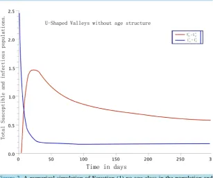
When the age structuring is considered, the dynamics of the host population in the U-shaped valleys is re- presented on Figure 1. When there is no age structuring, the dynamics for the U-shaped valleys are shown in

Figure 2. If we consider the U-shaped and the V-shaped valleys as one epidemiological region representing Western Kenya, then the dynamics are represented by Figure 3. The disease in the age structured model fades out faster. The steady states also settle to the endemic equilibrium faster.

If there is no spatialization the values for the U-shaped valleys for both ecosystems has host population vari- ation represented on Figure 3. The interaction between the patches raises infection rate, so that the disease per- sists in the total population, while it fades out fast when the patches are isolated.

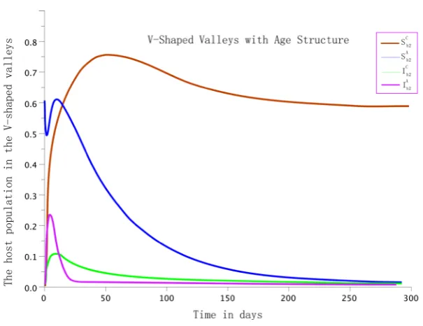
4.2. The V-Shaped Valley Sites: Fort Tenan and Marani, 0 = 1.67

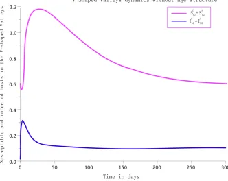
The dynamics of the model in the V-shaped valleys sites with age structure is given byFigure 4. When the age structuring is ignored the variation of the host population in the V-shaped valleys is represented by Figure 5.

5. Conclusions

[image:9.595.180.416.389.722.2]

Highland malaria in Western Kenya remains a source of mortality and morbidity. Concerned efforts have been put in place by the stakeholders to bring the disease under control with less than expected results. This study

Table 1. Parameter values and ranges for System 1 and Equation (5) in [1].

Parameter U-Shaped valleys V-shaped valleys

C

a 0.52 0.42

A

a 0.15 0.12

1

C

b 0.011 0.08

1

A

b 0.011 0.08

2

C

b 0.048 0.24

2

A

b 0.024 0.018

C h

µ 0.079 0.059

A h

µ 0.033 0.033

v

µ 0.033 0.033

ν 0.000283 0.000283

12

C

m 0.08 0.08

21

C

m 0.08 0.08

12

A

m 0.5 0.5

21

A

m 0.5 0.5

12

v

m 0.02 0.02

21

v

m 0.02 0.02

C

γ 0.0035 0.0035

A

γ 0.0035 0.0035

h

Λ 0.04 0.04

v

Λ 0.13 0.07

C

N 1500 1500

A

[image:10.595.158.469.83.312.2]

Figure 1. A numerical simulation for the variation of the two age classes population using Equation (1) and parameter values defined in Table 1 for the U-shaped valleys system with ₀=5.36.

Figure 2. A numerical simulation of Equation (1) no age class in the population and

0=5.36

 .

captures important factors key to endemicity of of malaria in Western Kenya, which could direct control mea- sure and targets effectively.

[image:10.595.161.469.348.605.2]

[image:11.595.159.471.83.342.2]

Figure 3. The variation of the total population in the region, no age class and the two ecosystems are treated as a single U-shaped valley ecosystem.

Figure 4. A numerical simulation of model 1 using parameter values defined in Table 1 for the V-shaped valleys ecosystem with age structure. In this case ₀=0.96 1< .

fection of highland malaria, there are fewer deaths due to acquired immunity compared to children. We note that the populations settle to the endemic equilibrium faster than in the age-structured than in the unstructured sys- tem as shown in Figure 5, and the stable equilibrium is achieved faster in the structured than the unstructured system. Adding age structure allows age specific control strategies to reduce disease prevalence.

[image:11.595.165.468.365.598.2]

[image:12.595.147.480.91.355.2]

Figure 5. A numerical simulation of model 1 using parameter values defined in Table 1 for the V-shaped valleys ecosystem without age structure. In this case 0=0.96 1< , A numeri-

cal simulation of model 1 using parameter values defined in Table 1 for the V-shaped valleys ecosystem. The is no age structures in the populations. In this case ₀=0.96 1< .

dynamics. Intervention then can be done with guidance from the model.

A more comprehensive characterization of results would have to include other types of patches that may not be terraine related but have different epidemiological characteristics from the U-shaped and the V-shaped val- leys. Such patches could take care of cities like Nairobi, where human migration has transferred malaria, and central Kenya where the cool highland ecosystem is disturbed by creation of dams for irrigation, rice cultivation, climate change and migration of population to the economically endowed part of the county. Adding age struc- ture allows age specific control strategies to reduce disease prevalence.

We assumed that vectors migrate especially to nearby patches, and the migration parameters for hosts are con- stant, similar and independent of the compartment. For the compartments that are far apart, the migration of mo- squitoes is negligible and is set to zero, since the mosquitoes are only able to fly about 2 kilometers away.

An explicit formula for 0 is obtained, which although complex due to the infinite number of patches, can be used to explore the effects of the parameters of the model. This formula will allow theoretical exploration of the options and efficiency of targeted public health intervention policies. The example in the two ecosystems simplifies the expression for 0, which we use to simulate our model with some realistic data from Western Kenya. This parameter is inversely related to migration of the hosts between the patches. This implies that to re- duce 02, we have to i) administer effective treatment through provision of proper health care facilities in both

patches, ii) promote drug adherence, iii) reduce malaria drugs abuse through self administration to shorten the infectious period and arrest human to mosquito infection, hence increase the rate of recovery represented by γ .

pact of climate related factors to the resurgent epidemics. Resistance of vectors to ITNs and IRS is also an im- portant factor which may cause the disease to remain a menace in the region, not to mention the possibility of drugs resistance in human and possible emergence if new malaria strains.

So far, we have formulated an analytical and numerical analysis which is a foundation of more research and also applicable to other vector borne disease like chikungunya [20].

Acknowledgements

We wish to acknowledge of the Inria Metz, UMMISCO(IRD), the French Embassy in Nairobi and the university of Nairobi, Kenya, for their financial, logistic and moral, support during the writing of this article. We are very grateful to Dr. Githeko, KEMRI Kisumu for the great insight and literature he gave us during this study.

References

[1] Josephine, W.K., Gauthier, S. and Ogana, W. (2013) Formulation of a Vector SIS Malaria Model in a Patchy Envi-ronment with Two Age Classes. Applied Mathematics, 222, 4444.

[2] Diekmann, O., Heesterbeek, J.A.P. and Metz, J.A.J. (1990) On the Definition and the Computation of the Basic Re- production Ratio R0 in Models for Infectious Diseases in Heterogeneous Populations. Journal of Mathematical Biology, 28, 365-382. http://dx.doi.org/10.1007/BF00178324

[3] Diekmann, O. and Heesterbeek, J.A.P. (2000) Mathematical Epidemiology of Infectious Diseases in Mathematical and Computational Biology. Wiley Series,Hoboken.

[4] Van Den Driessche, P. and Watmough, J. (2002) Reproduction Numbers and Subthreshold Endemic Equilibria for Compartmental Models of Disease Transmission. Mathematical Biosciences, 180, 29-48.

http://dx.doi.org/10.1016/S0025-5564(02)00108-6

[5] Varga, R.S. (1962) Matrix Iterative Analysis. Prentice-Hall,Upper Saddle River.

[6] Thieme, H.R. (2009) Spectral Bound and Reproduction Number for Infinite-Dimensional Population Structure and Time-Heterogeneity. SIAM Journal on Applied Mathematics, 70, 188-211. http://dx.doi.org/10.1137/080732870

[7] Varga, R.S. (1960) Factorisation and Normalised Iterative Methods Boundary Problems in Differential Equation. Uni-versity of Wisconsin Press,Madison.

[8] La Salle, J.P. (1976) The Stability of Dynamical Systems. Society for Industrial and Applied Mathematics. Regional Conference Series in Applied Mathematics.

[9] Hirsch, M.W. (1982) Systems of Differential Equations that Are Competitive or Cooperative: I. Limit Sets. SIAM Journal on Mathematical Analysis, 13, 167-179. http://dx.doi.org/10.1137/0513013

[10] Berman, A. and Plemmons, R.J. (1994) Nonnegative Matrices in the Mathematical Sciences, Volume 9 of Classics in Applied Mathematics. Society for Industrial and Applied Mathematics (SIAM), Philadelphia.

[11] Hirsch, H.W. and Smith, H.L. (2005) Monotone Dynamical Systems. In: Handbook of Differential Equations: Ordi-nary Differential Equations, Vol. II, Elsevier B. V., Amsterdam, 239-357.

[12] Chitnis, N., Hyman, J.M. and Cushing, J.M. (2008) Determining Important Parameters in the Spread of Malaria through the Sensitivity Analysis of a Mathematical Model. Bulletin of Mathematical Biology, 70, 1272-1296.

http://dx.doi.org/10.1007/s11538-008-9299-0

[13] Githeko, A.K., Branding-Bennet, D., Beier, M., Atieli, F., Owaga, M. and Collins, F.H. (1992) The Reservoir of Plas-modium Falciparum Malaria in a Holoendemic Area of Western Kenya. Transactions of the Royal Society of Tropical Medicine and Hygiene, 86, 335-358.

[14] Ndenga, B., Githeko, A., Omukunda, E., Munyekenye, G., Atieli, H., Wamai, P., Mbogo, C., Minakawa, N., Zhou, G. and Yan, G. (2006) Population Dynamics of Malaria Vectors in Western Kenya Highlands. Journal of Medical Ento-mology, 43, 200-206. http://dx.doi.org/10.1603/0022-2585(2006)043[0200:PDOMVI]2.0.CO;2

[15] UNICEF (2010) Kenya Statistics. Technical Report, United Nation,New York City.

[16] Wanjala, C.L., Waitumbi, J., Zhou, G. and Githeko, A.K. (2011) Identification of Malaria Transmission and Epidemic Hotspots in the Western Kenya Highlands: Its Application to Malaria Epidemic Prediction. Parasites and Vectors, 4,

81. http://dx.doi.org/10.1186/1756-3305-4-81

[17] Balls, M.J., Bodker, R., Thomas, C.J., Kisinza, W., Msangeni, H.A. and Lindsay, S.W. (2004) Effect of Topography on the Risk of Malaria Infection in the Usambara Mountains, Tanzania. Transactions of the Royal Society of Tropical Medicine and Hygiene, 98, 400-408.

Attrac-tiveness of Kenyan Men to the African Malaria Vector Anopheles Gambiae. Malaria Journal, 1, 17.

http://dx.doi.org/10.1186/1475-2875-1-17

[19] Smith, D.L., Guerra, C.A., Snow, R.W. and Simon, H.I. (2007) Standardizing Estimates of the Plasmodium falciparum

Parasite Rate. Malaria Journal, 6, 131. http://dx.doi.org/10.1186/1475-2875-6-131

currently publishing more than 200 open access, online, peer-reviewed journals covering a wide range of academic disciplines. SCIRP serves the worldwide academic communities and contributes to the progress and application of science with its publication.