Munich Personal RePEc Archive
Sectoral Shift, Wealth Distribution, and
Development
Yuki, Kazuhiro
Faculty of Economics, Kyoto University
30 May 2007
Online at
https://mpra.ub.uni-muenchen.de/3384/
Sectoral Shift, Wealth Distribution, and Development
Kazuhiro Yuki∗
forthcoming inMacroeconomic Dynamics
May 2007
Abstract
There are two phenomena widely observed when an economy departs from an underdeveloped
state and starts rapid economic growth. One is the shift of production, employment, and
consumption from the traditional sector to the modern sector, and the other is a large increase
in educational levels of its population. The question is why some economies have succeeded
in such structural change, but others do not. In order to examine the question, an OLG
model that explicitly takes into account the sectoral shift and human capital accumulation as
sources of development is constructed. It is shown that, for a successful structural change, an
economy must start with a wealth distribution that gives rise to an adequate size of ’middle
class’. Once the economy initiates the ’take-off’, the sectoral shift and human capital growth
continue until it reaches the steady state with high income and equal distribution. However,
when the productivity of the traditional sector is low, irrespective of the initial distribution and
the productivity of the modern sector, it fails in the sectoral shift and ends up in one of steady
states with low income and high inequality. Thus, sufficient productivity of the traditional
sector is a prerequisite for development.
JEL Classification Number: O11, O15.
Keywords: Human capital; Sectoral shift; Structural change; Wealth distribution
∗Faculty of Economics, Kyoto University, Yoshida-hommachi, Sakyo-ku, Kyoto, 606-8501, Japan; Phone
1 Introduction
There are two phenomena widely observed when an economy departs from an underdeveloped state
and starts rapid economic growth. One is the shift of production, employment, and consumption
from the traditional sector, such as traditional agriculture in rural areas and the urban informal
sector, to the modern sector, such as modern manufacturing and commercial agriculture. The other
is a large increase in educational levels of its population.1 Because the modern sector requires a
larger pool of skilled labor, it is easy to see that these phenomena are related. The question is why
some economies have succeeded in such ‘structural change’, but others do not. In order to tackle
the question, particularly regarding contemporary developing economies, this paper constructs an
OLG model that explicitly takes into account the sectoral change and human capital accumulation
as sources of development.
It is shown that, for a successful structural change, an economy must start with a wealth
distribution that gives rise to an adequate size of ’middle class’. Once the economy initiates the
’take-off’, the sectoral shift and human capital growth continue until it reaches the steady state
with high income and equal distribution. However, when the productivity of the traditional sector
is low, irrespective of the initial distribution and the productivity of the modern sector, it fails in
the sectoral shift and ends up in one of steady states with low income and high inequality. Thus,
sufficient productivity of the traditional sector is a prerequisite for development.
The model economy has two sectors, traditional and modern, each producing a different kind of
final good. The traditional sector hires unskilled labor and the modern sector employs skilled labor
and physical capital to produce the goods.2 The market of the good produced in the traditional
sector is closed domestically,3 while the market of the good produced in the modern sector, which
is also used as a capital good, and the factor market of physical capital are open internationally.4
An agent in the economy lives for two periods. In childhood, she receives a transfer from the
parent and allocates it between two investment opportunities, assets and education, in order to
maximize future income. The investment in education is required to become a skilled worker and
is individually profitable, although it is costly. The cost of education is the cost of hiring skilled
workers as teachers. Since loan markets are nonexistent, tuition must be self-financed.
Conse-1Empirical facts on the sectoral shift are summarized in Syrquin (1988) and those on the education growth are
surveyed in Schultz (1988).
2This assumption is made for simplicity. As long as the modern sector is more intensive in skilled labor, main
results remain unchanged.
3The traditional sector corresponds to traditional agriculture and the urban informal sector in a real economy,
which can be considered as nontradable sectors. See Section 2.3 for more detailed explanations.
4Perfect mobility of physical capital is assumed, mainly because it is more realistic than the other extreme of the
quently, poor parents cannot make investments in educating their children despite its profitability,
hence the investment decisions are affected by family income. In adulthood, the agent has a single
child, earns income from work and assets, and spends on the consumption of the two goods and
the intergenerational transfer.
The initial situation is that a large portion of the population is in the traditional sector and
remains unskilled. Because there is little room left for growth in the traditional sector, in order to
raise the standard of living significantly, the economy must accomplish the relocation of resources
from the traditional sector to the modern sector. More individuals must be educated, but many
of them are credit constrained and cannot make optimal investments. Under what conditions can
such economy succeed?
A part of the answer is that, as mentioned earlier, the economy must start with an initial
wealth distribution that gives rise to an adequate size of ’middle class’ (those who have enough
wealth to take education). The requirement for the ’take-off’ is that a portion of unskilled workers
accumulates wealth sufficient for their children to take education and get skilled jobs in the modern
sector. The source of labor income of unskilled workers is sales of the good produced in the
traditional sector. Its relative price in turn depends positively on the number of skilled workers
and aggregate assets: a higher number of skilled workers implies higher demand and lower supply
of the good, and greater wealth leads to the higher demand. Thus, for the sectoral shift to start,
the size of ’middle class’ and aggregate assets must be above certain levels.
If the initial wealth distribution is such that a relatively large portion of the population has
access to education and becomes skilled workers, the price of the traditional good and thus the
unskilled wage are high. If the price level is above the critical level, a richer portion of unskilled
workers can send their children to school and the sectoral shift starts immediately. Even when the
initial price level is not high enough for the shift due to modest aggregate assets, the relatively
large pool of skilled workers makes rapid wealth accumulation possible, hence the price level rises
to the critical level at some point and the economy ’take offs’. Once the sectoral change starts, it
continues autonomously. An increase in the number of skilled workers raises the demand for the
good, reduces its supply, and stimulates asset accumulation. All contribute to further increases in
the price of the good and the unskilled wage. This allows children of less affluent unskilled workers
to access education and thus increases the number of skilled workers further, lifting the price and
the unskilled wage even more. As long as the skilled wage (net of the cost of education) is higher
than the unskilled wage, this process continues. In the long run, the economy reaches the state
attained.5
In contrast, if the economy starts with a relatively small size of ’middle class’, the number of
skilled workers is limited, hence the price of the traditional good is low. Children of unskilled
workers are not able to access education financially and the number of skilled workers does not
increase. If initial wealth is low, the relative price increases over time through wealth accumulation
but never reaches the critical level for the sectoral shift. Because skilled labor remains scarce,
even in the long run, inequality between skilled and unskilled workers does not disappear and the
investment choices are affected by family income.
However, a ’good’ initial wealth distribution isnot sufficient for the success when there is the
sectoral shift of consumption, i.e. preferences are such that the income (and price) elasticity of
demand for the traditional good is less than one, while those for the modern good and the transfer
are more than one. If the productivity of the traditional sector is low, the economy ends up in a
steady state with persistent inequality irrespective of the initial distribution and the productivity
of the modern sector. Thus, sufficient productivity of the traditional sector is a prerequisite for
the successful development. Because the price elasticity of the traditional good is less than one,
when the productivity of the sector is lower, its price becomes higher more than proportionately
and the unskilled wage rises. The resultant lower return from education implies that the economy
can sustain fewer skilled workers and lower aggregate assets. If the productivity is below a certain
level, the sustainable skilled labor and aggregate assets become smaller than the levels required for
the ’take-off’ and thus the sectoral shift does not start.
The argument so far has assumed time-invariant productivities for the both sectors. The above
results are not largely affected by the introduction of productivity growth, as long as the cost of
education increases with the skilled wage. An economy starting with an unproductive traditional
sector is still unlikely to succeed in the structural change, irrespective of initial wealth distribution
and modern sector productivity. A new possibility is that an economy initially experiencing sectoral
shift may end up in a steady state with moderate income and high inequality, if wealth is relatively
concentrated in the rich.
The paper has several policy implications. The most important one would be that, when the
productivity of the traditional sector is low, policies enhancing the productivity and those correcting
wealth inequality (or lowering the private cost of education) must be conductedtogether. However,
the former policies should be executed with great care, because they have negative effects on the
unskilled wage, transfers by unskilled workers, and thus the upward mobility of their descendants.
5Larson and Mundlak (1997) finds that the ratio of average labor productivity of agricultural workers to that
The priority between the two kinds of policies depends on the productivity level and the stage of
development.
Empirical findings largely support the model’s implications. The first point of the paper, the
importance of initial wealth distribution, especially the initial size of ’middle class’, in economic
development, through its effect on human capital accumulation, has been backed by many studies.
Using panel data of wider coverage and of higher quality than those of earlier studies, Deininger
and Squire (1998) and Deininger and Olinto (2000) discover that an economy’s growth rate is
affected negatively by initial land inequality (a proxy for initial asset inequality) and positively by
its mean years of schooling per working person (a proxy for human capital).6 Further, they find
that the average educational attainment is negatively affected by initial land inequality, the effect
of human capital is greater in a lower-income economy, and initial land and income inequality affect
negatively the income growth of the poor, but not of the rich. Using cross-sectional data from the
1960s to the 1990s, Easterly (2001) finds that a larger size of ’middle class’, measured as the share
of income held by the second through fourth quintiles of the distribution, is associated with more
education, especially at the secondary level, higher income, and higher growth.
The second point of the paper, sufficient productivity in the traditional sector as a precondition
for a successful sectoral shift, has not been formally tested, although there are several findings
indirectly supporting the claim. Bairoch (1975) points out the large gap (about 45 percent) in
agricultural productivity on average between European countries at the onset of their industrial
revolutions and Africa and Asia in the 1960s. Further, Hayami and Ruttan (1985) finds a close
positive association between overall output growth and agricultural productivity growth for
Sub-Saharan African nations.
This paper is mainly related to two strands of literature. One is the literature that investigates
mechanisms and consequences of structural change. Matsuyama (1992) investigates the role of
agricultural productivity in economic development using a two-sector endogenous growth model and
shows how the openness of markets affects the relationship between productivity and growth. Using
a neoclassical growth model with multiple consumption goods and non-homothetic preferences,
Echevarria (1997) numerically shows that uneven productivity growth among sectors can lead to
different aggregate growth rates at different stages of development. Kongsamut et al. (2001) and
Ngai and Pissarides (2004) study multi-sector growth models related to the one investigated by
Echevarria and derive conditions for structural change and balanced growth. Laitner (2000) explains
how an economy’s measured average propensity to save rises in the course of industrialization by
focusing on the increasing importance of reproducible capital relative to land. Wang and Xie (2004)
6Unless aggregate wealth accumulation is very low, a more equal wealth distribution implies that a larger
examine factors affecting the activation of a modern industry based on a static two-sector model
with non-homothetic preferences and uncompensated spillovers in the IRS modern sector. These
papers as well as the present paper focus on sectoral shifts in the modern growth era. By contrast,
Hansen and Prescott (2002) are concerned with the transition from stagnation to modern economic
growth during past several hundred years in contemporary developed economies. Based on a
two-sector OLG model, they argue that the adoption of less land-intensive production technology
induced by productivity growth is the main driving force.
The other is the large literature that investigates the interplay between income distribution
and growth theoretically, which includes Banerjee and Newman (1993), Galor and Zeira (1993),
Ljungqvist (1993), Persson and Tabellini (1994), Benabou (1996a, 1996b), Benhabib and Rustichini
(1996), Aghion and Bolton (1997), Lloyd-Ellis and Bernhardt (2000), and Galor and Moav (2004).
Most closely related is the paper by Galor and Zeira, which shows how credit constraint and
lumpy investment in human capital can create the interaction between initial distribution and
long-run output and inequality. They consider an economy composed of two sectors that are similar in
production technologies to the present paper but both produce the same tradable good. (Thus,
the sectoral shift of consumption is not considered.) In a version of the model with land as a
factor of production of the traditional sector,7 the unskilled wage and thus the upward mobility
of the poor depend on wealth distribution and the skilled wage, as in this paper. (They depend
on aggregate assets too in the present model.) However, the mechanism is different. In the Galor
and Zeira model, what gives rise to the dependency is a decreasing marginal return to labor in the
traditional sector and the credit constraint that individuals can borrow to finance education but at
a higher rate than the lending rate, which makes the number of borrowers and thus the number of
skilled workers affected by the return to education. In the present model, the dependency comes
from the endogenous relative price of the traditional good that reflects both demand and supply
factors. Further, with the sectoral shift of consumption, resources available to skilled workers also
depend on the relative price. In terms of policy implications, the most contrasting would be effects
of policies improving access to education through transfers to the poor. In their model, irrespective
of the productivity level of the traditional sector, such policies are sufficient for an economy to
escape from the state of low output and high inequality. By contrast, in the present model with
the sectoral shift of consumption, when the productivity is low, such policies must be implemented
together with the productivity-enhancing policies.
Galor and Moav construct a one-sector OLG model related to that of Galor and Zeira, in order
to explain the transition of the main engine of growth from physical capital accumulation (in early
7Footnotes 11, 19, and 26 discuss a modified model where land is included as in the Galor and Zeira model.
stages of the Industrial Revolution) to human capital accumulation (in the modern growth era).
Further, they show that the effect of inequality on growth turns from positive to negative with the
replacement of the prime source of growth.
The paper is organized as follows. Section 2 presents the model without the sectoral shift of
consumption. Section 3 derives and analyzes the model’s dynamics and Section 4 presents and
interprets the results from the basic model. In Section 5, the sectoral shift of consumption is
introduced into the model and its effects on the results are examined. Further, policy implications
of the model are discussed. Section 6 concludes the paper.
2 Model
2.1 Individual decisions
Time is discrete and starts from 0. There is no uncertainty. The economy is composed of a
continuum of individuals who live for two periods.
2.1.1 Investment decisions
In childhood, an individual receives a transfer from her parent and allocates it for two investment
options, assets and education, in order to maximize future income.8 Education, which would
correspond roughly to secondary education in actual developing economies, is required to become
a skilled worker and enjoy higher earnings in adulthood. The investment is a discrete choice, i.e.
takes education or not, and incurs a fixed cost. Consider an individual who was born into lineage
i in period t−1, whose generation is called generation t. Her education costs et, and its gross
return is wH,t− wL,t in the next period, where wH,t and wL,t are skilled and unskilled wages in
period t, respectively. Assume that the education cost is the cost of hiring current skilled workers
as teachers and it is proportional to wH,t−1, i.e. et = sewH,t−1, where se is a constant.9 The
investment must be self-financed because loan markets for such investment are not available: the
child’s future income is not a valid collateral in the financially underdeveloped economy. The other
option, the investment in assets, is a continuous choice, and brings a gross rate of return of 1 +rt.
It is easily shown that, in an equilibrium, the return from the educational investment becomes at
least as high as the return from the investment in assets, i.e. wH,t−wL,t ≥(1 +rt)et.
8Alternatively, one can suppose that the investment decisions are carried out by the parent in order to maximize the
child’s future income. Note that the transfer in the model corresponds to total intergenerational transfers including bequests, education, and other inter-vivos transfers in real life. The decision that the child (or the parent) has to make is the allocation of the whole transfers between education and assets.
9Kendrick (1976) finds that teacher and student time constitute about 90% of all costs of education. Further,
Suppose that the individual has receivedbi
tunits of income as a transfer from the parent. If the
return from the investment in education is strictly higher than that from the investment in assets,
optimal investment choices of assetsai
t and educationeit are given by the following equations:10
If bi
t< et, ait=bit, eit= 0, (1)
and if bi
t≥et, ait=bti−et, eit=et. (2)
Since innate abilities of individuals are identical, transfers solely determine the investment and
resulting occupational choices.
2.1.2 Consumption and transfer decisions
An adult individual, who is either a skilled or unskilled worker depending on the human capital
investment in the previous period, obtains income from assets and labor supply and spends the
income on consumption and transfer to her child. Each adult is assumed to have a single child.
There are two different consumption goods, good L and good H. Characteristics of the goods are
described later in this section. Assume that an adult individual of lineageiin generationthas the
following utility function:
Uti = (c i
L,t) γl(ci
H,t) γh(bi
t+1)1−γl−γh, (3)
whereci
L,t andciH,tare her consumption of good L and good H, respectively andbit+1is the transfer
to the child (generation t+ 1). Denote the relative price of good L to good H in period t by Pt.
Then, the budget constraint is (wi
t is her earnings)
PtciL,t+c i
H,t+b i
t+1 =wit+ (1 +rt)ait. (4)
Maximization of (3) subject to (4) gives the following consumption and transfer rules:
PtciL,t =γl[wti+ (1 +rt)ait], (5)
ciH,t =γh[w i
t+ (1 +rt)ait], (6)
and bit+1 = (1−γl−γh)[w
i
t+ (1 +rt)ait]. (7)
10Actually, the relative return from education is determined as the result of people’s investment decisions, since
2.1.3 Generational structure
At the beginning of period t+ 1, current adults pass away, current children become adults, and
new children are born into the economy. Since each adult has one child, the population is constant
over time. The population of each generation is normalized to be one.
2.2 Production structure
There are two production sectors, sector L (the traditional sector) and sector H (the modern sector).
Sector L employs unskilled workers to produce good L, and sector H employs skilled workers and
physical capital to produce good H. Good H is used for investment in physical capital as well.
The production functions of the two sectors are given as follows:
Sector L: YL,t=AL,tLt, (8)
Sector H: YH,t=AH,t(HH,t)α(Kt)1−α, 0< α <1. (9)
In the above expressions, YL,t and YH,t are outputs of good L and good H, respectively, AL,t and
AH,tare productivity levels of the respective sectors, Ltis the number of unskilled workers, HH,t is
the number of skilled workers in sector H (the rest of skilled workers are employed in the education
sector), andKtdenotes physical capital.11 To focus on main mechanics of the model, in most parts
of the paper, the productivitiesAL,tandAH,t are assumed to be constant over time, i.e. AL,t=AL
and AH,t=AH. As described later, main results remain intact with the introduction of exogenous
productivity growth.
The assumptions that unskilled workers are employed only in sector L, and skilled workers and
physical capital are employed only in sector H are made for simplicity. Provided that the former
sector is more intensive in unskilled labor and the latter sector is more intensive in skilled labor,
the outcome from the model remains largely unchanged.
2.3 Market structure and determination of prices
Suppose that the markets for good L and for labor are closed domestically, while good H and
physical capital are freely mobile internationally. The assumptions on the final goods would be
better understood by associating them with goods in an actual economy.
The first interpretation is that good L is agricultural goods produced with traditional technology,
and good H is manufacturing and agricultural goods produced with modern technology. Traditional
11As mentioned in the introduction and explained in the next subsection, sector L corresponds to the urban informal
sector as well as traditional agriculture in a real economy, hence land is not included in the production function. If land is a factor of production, the production function may be formulated as: YL,t =AL,t(Lt)β(Z)1−β, 0< β <1,
agriculture is engaged on a small scale by families located in rural areas and produces agricultural
goods largely for basic needs. Because its productivity is low and transportation costs and traders’
margins are high due to poor infrastructure and distribution system,12 it supplies the product
mostly for domestic markets. By contrast, modern manufacturing and commercial agriculture
compete more directly with foreign suppliers.
The second interpretation is that good L is non-tradable services and manufacturing goods
produced with technologies intensive in unskilled labor, such as petty trading, personal services,
and repairing services, and good H is manufacturing goods produced with technologies intensive in
skilled labor and physical capital. That is, sector L and sector H may be considered as the informal
and formal sectors of an urban economy, respectively. There is an evidence showing that the size
of the urban informal sector is substantial in most developing countries, in many cases accounting
for over half of the urban workforce (Ranis and Stewart, 1999).13
Perfect mobility of physical capital is assumed, because it is more realistic than the other
extreme of the closed market as a description of the situation of contemporary developing economies,
and it enables the paper to focus on human capital accumulation rather than physical capital
accumulation as the prime source of development.
From the assumptions, the interest rate is fixed at the world interest rate rt = r, which is
assumed to be time-invariant, and the skilled wage wH is given by the following equation.14
wH =α(AH)
1
α(1−α
r
)1
α−1. (10)
The wage rate is exogenous and constant over time. The wage of unskilled workers equals
wL,t=PtAL, (11)
hence it depends on the relative price of good L to good H, Pt.
12See, for example, Minten and Kyle (1999) for an evidence from former Zaire.
13Of course, in a real economy, there exist skill-intensive sectors that supply nontradable services and goods.
However, in lower developing countries, most of skill-intensive nontradables are public services, health services, and education, where service prices and wages are determined more by institutional factors than by market conditions, while nontradable sectors influenced more directly by market factors, such as financial services and consulting services, are limited in size. By comparison, as explained in the main text, traditional agriculture and the urban informal sector are important parts of unskilled-intensive sectors in developing countries. Hence, the assumption on the tradability of the two final goods would be justified. Note that, as mentioned in the previous subsection, the assumption that sector H employs only skilled labor and physical capital and sector L employs only unskilled workers can be relaxed without affecting main results largely.
14From the first-order conditions of the profit-maximizing problem of the firm in sector H,
rt= (1−α)AH
“HH,t
Kt ”α
,
and wH,t=αAH
“ Kt
HH,t ”1−α
.
Solving the first equation for HH,t
The relative price is determined by the market-clearing condition of good L. The demand for
good L is the total consumption of the good by the adult population, which is the sum of individual
consumption (5) over the population. So the market-clearing condition becomes
PtALLt=γl
[
wL,tLt+wHHt+ (1 +r)
∑ i ai t ] . (12)
In the above equation,Htis the total number of skilled workers, which is the sum ofHH,t andHE,t
(the number of skilled workers in the education sector), and ∑iai
t is aggregate assets. Note that,
due to free international capital mobility, it could be the case that a large portion of the assets
are invested abroad, if there do not exist enough investment opportunities within the economy. By
substituting (11) and Ht+Lt= 1 into the above equation and solving forPt,the relative price of
good L is given as follows:
Pt=
γl 1−γl
wHHt+ (1 +r)
∑
ia i t
AL(1−Ht)
. (13)
The relative pricePtincreases with the number of skilled workers Htand aggregate assets. Larger
Htand
∑
ia i
t imply greater total income and higher demand of good L, and largerHt(smaller Lt)
implies lower supply of the good, hence higher Pt. Since wL,t =PtAL, the unskilled wage is also
increasing in Ht and
∑
ia i t.
For analyses in later sections, it is convenient to express the relative price as a function of Ht
and aggregate intergenerational transfers, Bt, by substituting
∑
ia i
t = Bt−eHt into the above
equation (13):15
Pt=
γl 1−γl
[wH−(1 +r)e]Ht+ (1 +r)Bt
AL(1−Ht)
. (14)
The relative price and the unskilled wage are increasing in bothHtand Bt. To express the
depen-dency of Pt and wL,t on Ht andBt, they are denoted asP(Ht, Bt) and wL(Ht, Bt),respectively.
The education sector employs skilled workers as teachers to provide educational services to
students. Since tuition equalseand the number of students isHt+1in periodt, the market-clearing
condition is
wHHE,t =eHt+1, (15)
or HE,t =seHt+1. (16)
The above equation shows that the constantse represents the number of teachers needed to teach
one student. It is assumed thatse <1 is low enough that the above condition is satisfied without
15The relationP
ia i
t=Bt−eHt is satisfied because current skilled workers have spenteon education out of their
rationing: otherwise, not all children who have enough wealth to pay tuition could receive education
because of a shortage of teachers.
3 Dynamics
In the model economy, individuals live only for two periods and participate in each market for one
period alone: each market consists of individuals of a single generation each period. Hence, the
model can be considered as a sequence of static economies.
What connects these static economies across periods are intergenerational transfers. Because
of the credit constraint, transfers directly affect individuals’ investment and occupational choices,
and consequently consumption and transfer decisions. Further, the distribution of transfers over
the population determines the proportion of individuals who can afford to take education, and
thus it affects the relative return from education and investment decisions. Hence, in general, the
time evolution of the distribution of transfers must be examined in order to understand how the
economy’s structure, such as production and employment shares of each sector, total output, and
wage and asset distributions, change over time.
This section first derives the dynamic equation linking the current period’s transfer to the
next period’s transfer within a lineage (individual dynamics). The dynamics depend on the time
evolution of two aggregate variables that in turn are determined by the dynamics of the distribution
of transfers. However, it turns out that, sufficient information for obtaining the model’s implications
is the directions of motion of the aggregate variables, which can be derived without knowledge on
the distributional dynamics. Thus the dynamics of the two aggregate variables are examined next.
Although the two dynamics interact, for exposition, initially the dynamics of each variable are
analyzed fixing the other, then the both dynamics are analyzed together by introducing a phase
diagram.
3.1 Individual dynamics
Consider an individual born into lineageiin periodt−1, who belongs togeneration t. She allocates
transfer bi
t between investments in assets ait and in education eit so as to maximize future income.
If the transfer is less than the cost of education, i.e. bi
t < e, the transfer is spent only on assets
and she becomes an unskilled worker, as described earlier. By contrast, if bi
t ≥ eis satisfied, the
investment decision is more complicated. Because investment decisions of others affect wL(Ht, Bt)
and the relative return from education, she has to take into account their actions. The key variable
affecting the decision is the fraction of individuals with bi
t ≥ e, Ft. In short, when only a small
when many individuals have access to education, some of them become unskilled workers and the
wages (net of the cost of education) are equalized.
3.1.1 Unequal opportunity case
When the proportion of individuals who can afford to take education is small, the return from
education is higher than the return from assets, even if all of them take education, i.e. wH−(1+r)e >
wL(Ft, Bt). In this case, the individual allocates the transfer in the following manner:
If bi
t< e, a i t=b
i t, e
i
t= 0, (17)
and if bi
t≥e, a i t=b
i t−e, e
i
t=e. (18)
Thus, all young individuals who are financially eligible for education become skilled workers, i.e.
Ht = Ft. Since transfers from parents constrain access to the profitable investment opportunity,
this case is called the unequal opportunity case.
In the next period, the individual, given asset ai
t and acquired ability (skilled or unskilled),
determines the amount of transfer to the child bi
t+1 according to (7). By substituting the above
investment rules into (7), the dynamic equation linking the received transferbi
tto the transfer given
to the next generationbi
t+1 is derived.
If she is a skilled worker, i.e. bi
t≥e, the equation takes the following form:
bi
t+1 = bs(bit)≡(1−γl−γh){wH+ (1 +r)(b
i
t−e)}. (19)
The assumption (1−γl−γh)(1 +r) < 1 is made so that the fixed point of the equation (bs)
∗ ≡
1−γl−γh
1−(1−γl−γh)(1+r)[wH−(1 +r)e] is stable.
For an unskilled worker, i.e. bi
t< e, the equation becomes
bit+1=bu(bti;Ft, Bt)≡(1−γl−γh){wL(Ft, Bt) + (1 +r)bit}, (20)
where wL(Ft, Bt) =
γl 1−γl
[wH−(1 +r)e]Ft+ (1 +r)Bt
(1−Ft)
. (21)
The dynamic equation for an unskilled worker does depend on the aggregate variablesHt=Ftand
Bt, because they affect the relative price of good L and thus the unskilled wage. The fixed point
forgiven Ft and Bt is denoted byb∗u(Ft, Bt)≡ 1−(1−1−γγl−γh
l−γh)(1+r)wL(Ft, Bt).
16
The dynamics of a current skilled worker,bi
t+1 =bs(bit) and of a current unskilled worker,bit+1=
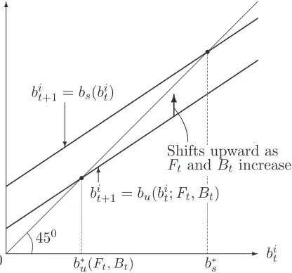
bu(bit;Ft, Bt), for given Ftand Btare depicted in Figure 1.17 As long aswH−(1 +r)e > wL(Ft, Bt)
16This maynot be the long-run transfer level of her lineage, because her descendants may become skilled workers
and FtandBtcould change over time. One might think that this fixed point does not have any economic importance,
but it turns out that the level ofb∗
u(Ft, Bt) is crucial for aggregate dynamics (detailed later).
17To be more accurate, bi
✲ ✻ ¡¡ ¡¡ ¡¡ ¡¡ ¡¡ ¡¡ ¡¡ ¡¡ ¡¡
0 bit
bi t+1 ✑✑ ✑✑ ✑✑ ✑✑ ✑✑ ✑✑ ✑✑ ✑✑ ✑✑ ✑✑ ✑✑ ✑✑ ✑✑ ✑✑ ✑✑ ✑✑ ✑✑ ✑✑ r r b∗
u(Ft, Bt) b ∗ s
bi
t+1 =bs(bit)
❄
✻
bi
t+1=bu(bit;Ft, Bt)
450
✻
Shifts upward as
[image:15.595.212.420.38.232.2]Ft and Bt increase
Figure 1: Individual dynamics of intergenerational transfers
is satisfied, bi
t+1 =bu(bit;Ft, Bt) is located belowbit+1 =bs(bit),but it shifts upward with increases
inFt and Bt.
3.1.2 Equal opportunity case
Next, consider the case in which many individuals can afford education so that the return from
education fails to be higher than the return from assets, if all of them invest in education, i.e.
wH−(1 +r)e≤wL(Ft, Bt). In this situation, the number of skilled workersHtis determined at the
point where the two returns are equated, i.e. wH−(1 +r)e=wL(Ht, Bt). Nownot all of financially
eligible individuals take education and become skilled workers, i.e. Ht≤Ft. Since the return from
the investments does not depend on transfers from parents, this case is named theequal opportunity
case. Dynamics of transfers of the both types of workers are described by bi
t+1 =bs(bit), (19). In
Figure 1, this is the situation where P(Ht, Bt) is high enough that bit+1 = bu(bit;Ht, Bt) coincides
withbi
t+1 =bs(bit).
3.1.3 Dividing line
The economy belongs to either of the two cases depending on Ft and Bt. The combination of Ft
and Btsatisfying wH−(1 +r)e=wL(Ft, Bt) is the dividing line, which is obtained by substituting
Pt= [wH−(1 +r)e]/AL,
∑
iait=Bt−eHt, and Ht=Ft into (13) and solving forFt:
Ft=He(Bt)≡(1−γl)−
γl(1 +r)Bt
wH−(1 +r)e
. (22)
since the location oferelative tob∗
u(Ft, Bt) depends onFt andBt,eis not shown in the figure. Precise dynamics of
The unequal opportunity case corresponds to Ft < He(Bt), while the equal opportunity case
amounts toFt≥He(Bt) =Ht.
3.2 Aggregate dynamics
What has become clear now is that the individual dynamics and the evolution of wages and the
relative price depend on the dynamics of two aggregate variables, aggregate transfers Bt and the
fraction of individuals satisfyingbi
t≥e,Ft. Given the initial distribution of transfers,B0andF0are
determined directly, while levels of the aggregate variables in subsequent periods are determined
by the dynamics of the distribution of transfers. However, as mentioned earlier, information on
thedirection of motion of the aggregate variables, which can be derived without knowledge on the
distributioal dynamics, is enough to obtain main implications of the model. Thus, this
subsec-tion analyzes the dynamics of Bt and Ft qualitatively. For exposition, each of them is examined
separately fixing the other variable first, then their interaction is taken into account at the end.
3.2.1 Dynamics of aggregate transfers
First, the dynamics of aggregate intergenerational transfersBtare examined forgiven Ft. Consider
the unequal opportunity case, i.e. Ft< He(Bt). As seen in the previous subsection,wH−(1+r)e >
wL(Ht, Bt) andHt=Fthold in this case. The dynamic equation of aggregate transfers is
Bt+1 =B(Ft, Bt)≡
1−γl−γh 1−γl
{[wH−(1 +r)e]Ft+ (1 +r)Bt}, (23)
which is derived by aggregating individual dynamics of skilled (19) and of unskilled workers (20)
over the population and substitutingHt=Ft. The assumption 1−1−γl−γγh
l (1 +r)<1 is made so that there exists a fixed point that is globally stable for given Ft, where the fixed pointB∗(Ft) equals
B∗
(Ft)≡ 1
1−1−1γl−−γlγh(1+r)
1−γl−γh 1−γl
[wH−(1 +r)e]Ft. (24)
Alternatively, in the equal opportunity case (Ft ≥ He(Bt)), wH−(1 +r)e = wL(Ht, Bt), i.e.
Ht=He(Bt),holds. In this case, the dynamic equation is obtained by substituting Ht=He(Bt)
intoBt+1 =B(Ht, Bt):
Bt+1 =B(He(Bt), Bt)≡(1−γl−γh){[wH−(1 +r)e] + (1 +r)Bt}. (25)
Note that the equation does not depend on Ft. The fixed point of the equationB∗∗ is
B∗∗
= 1−γl−γh
✲ ✻ ¡¡ ¡¡ ¡¡ ¡¡ ¡¡ ¡¡ ¡¡ ¡¡ ¡¡ 450
0 bit
bi t+1 s ❝ ✸ ✰ ✸ ✰ s s b∗
u(Ft, Bt) b
∗ s
e e
bi
t+1=bs(bit)
❄
✻
bi
[image:17.595.209.408.37.231.2]t+1 =bu(bit;Ft, Bt)
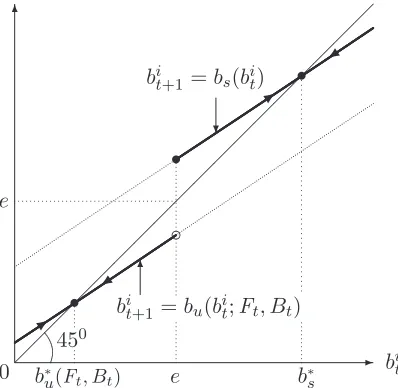
Figure 2: Unequal opportunity case whenb∗
u(Ft, Bt)≤e
which is equal to (bs)∗ and globally stable. And the number of skilled workers at B∗∗, H∗∗ ≡
He(B∗∗), equals
H∗∗
≡He(B∗∗
) = (1−γl)− γl(1 +r)B
∗∗
[wH−(1 +r)e]
,
= 1− γl
1−(1−γl−γh)(1 +r)
. (27)
3.2.2 Dynamics of Ft
Next, the dynamics of Ft, the proportion of people who can afford education, are examined for
given Bt. Unlike aggregate transfers, the dynamic equation relating Ft to Ft+1 depends on the
distribution of transfers over the population, so it cannot be derived without complete information
on the distribution. However, the direction of change ofFt can be known only with current values
of the two aggregate variables, Bt and Ft.
Assume that(1−γl−γh)wH ≥e, i.e. B
∗∗ =b∗
s ≥e,is satisfied. Note that this assumption places
a restriction not on the productivity of sector H but on the degree of altruism. Since e= sewH,
it can be rewritten as 1−γl−γh ≥ se, which implies that people are altruistic enough towards
their children. From the assumption, Ft is non-decreasing over time, becausebit+1 ≥eis satisfied
whenever bi
t≥eis true (see Figure 2).
First, consider the unequal opportunity case, in which transfers of unskilled workers change
over time according to bi
t+1 =bu(bit;Ft, Bt). Whether Ft remains constant or increases over time
is determined by the relative size of b∗
u(Ft, Bt) to e. When b∗u(:)≤e, none of offspring of unskilled
workers receive transfers greater than e(bi
t< e impliesbit+1 < e), so Ft is constant (see Figure 2).
In contrast, whenb∗
u(:)> eis satisfied, Ft+1 ≥Ft holds, because, depending on the distribution of
✲ ✻
¡¡ ¡¡
¡¡ ¡¡
¡¡ ¡¡
¡¡ ¡¡
¡¡
450
0 bit
bi t+1
s
❝
✸
✰
✸
s
q
b∗
u(Ft, Bt) b∗s
e e
bi
t+1=bs(bit)
❄
✻
bi
[image:18.595.209.409.36.232.2]t+1=bu(bit;Ft, Bt)
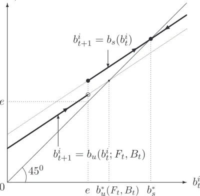
Figure 3: Unequal opportunity case whenb∗
u(Ft, Bt)> e
3). AndFt definitely increases in the longer term, whenb∗u(:)> e continues to hold for sufficiently
many periods. From (21), the dividing line b∗
u(Ft, Bt) =eis given by
Bt=
1−(1−γl−γh)(1 +r) (1−γl−γh)(1 +r)
1−γl
γl
e(1−Ft)−
[wH−(1 +r)e]Ft
1 +r . (28)
Alternatively, in the equal opportunity case, transfers of the both types of workers follow bi t+1 =
bs(bit), andFt+1 ≥Ftis satisfied.
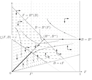
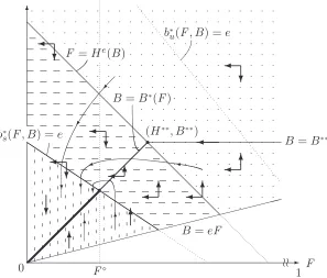
3.2.3 Joint dynamics of Ft and Bt
Finally, the dynamics ofFtandBtare analyzed together by introducing the phase diagram (Figure
4), in which the horizontal axis represents F and the vertical axis represents B.18,19 Feasible
combinations ofF andB are equal to the area bound byF = 0,F = 1,andB =eF.The economy
must satisfyB ≥eF, becauseF is defined as the fraction of individuals who have received transfers
bi greater than the cost of education e.
The diagram is divided into two regions, one corresponding to the unequal opportunity case
and the other region for the equal opportunity case (dotted area), by F = He(B), (22). The
region below the locus is the unequal opportunity case, where all the individuals who can afford
education take education and become skilled workers, i.e. H =F.The region above it is the equal
opportunity case, in which the number of skilled workers is determined so that the return from
18A more formal analysis of the dynamics of the aggregate variables is available from the author upon request.
19Even when sector L is interpreted as traditional agriculture and thus land is included in the production function
✲ ✻
0 F
B
B =B∗(F)
F =He(B)
✘✘✘✘✘✘
✘✘✘✘✘✘
✘✘✘✘✘✘
✘✘✘✘✘✘
B =eF b∗
u(F, B) =e
r
F†
tB =B∗∗ (H∗∗, B∗∗)
r
1
❄ ❄
✲
❄ ✲
❄
✲ ❄✲
✻
✻ ✻✲ ✲
✻ ✲
✻ ✲ ❄
✲
❘
q ❘
✿
❄ ❯
◆
✻ ✸
✿
[image:19.595.146.459.36.306.2]✻
Figure 4: Phase diagram
education is equated with the return from assets, i.e. H =He(B)≤F.
In the unequal opportunity case, the direction of motion ofB is determined by the position of
current (Ft, Bt) relative to B =B∗(F), (24). When the current economy is located on the line,Bt
is constant; when located above (below), it decreases (increases) over time. The direction of change
of B in each region is expressed with vertical arrows. As for the direction of change of F = H,
it is determined by the location of (Ft, Bt) relative to b∗u(F, B) = e. In the region below or on
the line (the area with vertical dashed lines), b∗
u(:) ≤ e is satisfied, accordingly Ft+1 =Ft holds;
in the region above the line (the area with horizontal dashed lines), b∗
u(:) > e, hence Ft+1 ≥Ft is
satisfied (andFtincreases in the longer term, if the economy stays in the region for sufficiently many
periods). Alternatively, in the equal opportunity case, the direction of motion of B is determined
by the relative location to B=B∗∗, (26), and F
t+1 ≥Ft always holds.
With this diagram, qualitative properties of transitional dynamics and the long-run outcome
of the aggregate variables (F, B) are transparent. Except when B > B∗(F), b∗
u(F, B) > e, and
F < H∗∗ are simultaneously satisfied, they are completely known only with the position of (F
t, Bt)
4 Analyses
4.1 Initial distribution and long-run economic structure
By using this diagram, the relationship between the initial distribution of wealth and the long-run
structure of the economy along with its transition can be easily investigated.
First, consider an economy that attains equal opportunity from the beginning, whose initial
position is in the dotted area of the diagram. Since returns from the two investment opportunities
are equated, the both types of workers earn the same level of earnings (net of the cost of education),
and education becomes affordable to children of poor unskilled workers over time (F increases).
As long as the economy starts withF0 >F† (F† is defined as the value ofF at the intersection of
b∗
u(F, B) =eandB =B∗(F)), it converges to (F, B) = (1, B∗∗) for certain, where not only the net
earnings but also net income and wealth are equalized andbi=b∗
sholds. That is,perfect equality is
attained. The long-run outcome of the economy withF0 ≤F†, by contrast, depends on the exact
initial distribution. If wealth is highly concentrated in the rich, F would increase only slightly and
the economy may regress to the unequal opportunity case (crosses the lineF =He(B
t)). Otherwise,
it would converge to (1, B∗∗).
Next, examine an economy that starts from the area with horizontal dashed lines. It does not
satisfy equal opportunity initially, but children of unskilled workers gain access to education over
time (F increases). Thus, the number of skilled workers increases and wage inequality between
skilled and unskilled workers diminishes. Associated with this change, production and employment
shares of sector H rise, while those of sector L fall. When F0 > F†, the economy attains equal
opportunity at some point and perfect equality is realized in the long run. On the other hand,
when F0 ≤F†, the long-run outcome depends on the exact initial distribution. If the distribution
is concentrated in the few rich, the number of skilled workers increases only slightly over time, and
it is possible that the economy crossesb∗
u(:) =e.
The remaining scenario is that an economy starts from the area with vertical dashed lines, where
not only investment opportunities are unequal but also children of unskilled workers cannot access
education, i.e. b∗
u(:)≤e. Since the number of skilled workers is constant, the sectoral composition of
production and employment remains unchanged. In particular, ifF0 ≤F†, the economy converges
to (F0, B∗(F0)), and unequal opportunity and inequality persist in the long run. If the economy starts with F0 >F†, its long-run prospect is much brighter. While asset accumulation is low, poor
people cannot afford education and hence the number of skilled workers remains constant. But,
after a certain amount of asset accumulation, the economy transits to b∗
u(:) > e and the sectoral
The analysis has shown that there is a clear-cut relationship between the initial distribution of
wealth and the attainment of the structural change and equal opportunity in the long run. That
is, if the initial distribution is such that the fraction of individuals who have enough resources
to take education is low, the economy remains stagnant. Thus, the initial size of ’middle class’
matters for development through sectoral change. Note that equal distribution does not always
lead to development: if initial aggregate wealth is very low, too equal wealth distribution implies
F0 ≤F† and results in stagnation. Further, if the economy starts below the critical level of asset
accumulation,B0=F†e, it remains stagnant irrespective of the initial distribution.
When productivity growth is introduced into the model, all the variables except F grow over
time even in the long run, but the qualitatively same phase diagram can be drawn, after the
non-stationary variables are adjusted for the productivity growth of sector H. Hence, all the qualitative
results in this subsection remain unchanged.20 Without the productivity growth, the sectoral shift
is necessarily associated with a rise of the relative price of good L, but now the relative price may
decrease over time if the productivity growth of sector L is large enough.
4.2 Comparisons among long-run equilibria
There are two kinds of steady state equilibria, (Fss, Bss) = (1, B
∗∗) and (F, B∗(F)), where F ≤F†.
In the former equilibrium, the number of skilled workers is H∗∗, the skilled wage (net of the cost
of education) is equal to the unskilled wage, and all individuals hold the same level of wealth,
1
1−γl−γh(bs)
∗.21 On the other hand, in the latter type of equilibria, the number of skilled workers is
F (≤F†< H∗∗), the (net) skilled wage is higher than the unskilled wage, and the wealth of skilled
workers, 1−γ1 l−γh(bs)
∗, is greater than that of unskilled workers, 1 1−γl−γhb
∗
u(F, B∗(F)). The relative
price of good L, P(H, B∗(H)), is increasing in H,so arewL(H, B∗(H)) andb∗
u(H, B∗(H)).
These steady state equilibria can be ranked in terms of the wage and wealth of unskilled workers,
which may be also interpreted as measures of inequality between skilled and unskilled workers,22
and of the total wealth of the economy.23 The best equilibrium is (1, B∗∗), then among equilibria
(F, B∗(F)),F ≤F†, one with larger F is better. The ranking, however, does not take into account
20 The detailed analysis is available from the author upon request. One thing to note is that both H∗∗ and F†
increase with the growth rate of sector H productivity. That is, with the faster productivity growth, the number of skilled workers and thus the size of sector H become greater in the equal opportunity steady state, but it becomes moredifficult for an economy with a small size of ’middle class’ to initiate the sectoral shift. Thus, the productivity growth of the modern sector enhancesthe disparity of the long-run outcome among economies with different initial conditions.
21Wealth is defined asw
H−(1 +r)e+ (1 +r)(bs)∗.
22Remember that the wage and wealth of skilled workers are same in all the steady state equilibria. Interestingly,
Deininger and Squire (1998) finds that initial land and income inequality affect negatively income growth of the poor, butnot of the rich.
23Total wealth at equilibrium (1, B∗∗) equals 1 1−γl−γh(bs)
∗, while at equilibria (F, B∗(F)),F <F†, it is equal to
1 1−γl−γh(bs)
∗ F
the fact that the relative price of good L is different across the equilibria. For accurate welfare
comparisons, the utility of each type of workers needs to be computed. Still, the ordering among
the steady state equilibria remains unchanged, if the average utility, which can be interpreted as
the expected utility of an individual before birth, is used for the comparison.24
4.3 Mechanism behind the results
The mechanism of the model yielding the above results can be explained intuitively by the following
illustration (see Figure 4). Consider an economy in which skilled workers are scarce (H0 =F0 <
H∗∗) and its asset accumulation is modest (B
0 < B∗(H0)) initially. How can this economy raise its income level? One route is through further asset accumulation. Many individuals leave more
than they received from parents to children. The growth of wealth raises the demand for good
L, its price, and the unskilled wage. The increased unskilled wage then stimulates savings by
unskilled workers, further promoting asset accumulation. This process continues until aggregate
assets reach the steady state level. However, with the number of skilled workers constant, the
income growth is moderate since the ultimate source of asset accumulation is labor income. Further,
inequality between skilled and unskilled workers remains large because the investment opportunities
are constrained by family income.
Thus, in order to attain large income growth, an increase in the number of skilled workers
and the sectoral shift of production and employment from sector L to sector H is crucial. The
sectoral shift starts iff a fraction of children of unskilled workers receive enough resources to take
education, which is possible when the unskilled wage wL,t = PtAL and thus the relative price of
good L are above critical levels. The relative price depends positively on the number of skilled
workers and aggregate assets: the demand for good L increases with the both variables, while its
supply decreases with the number of skilled workers. Hence the two variables must be above certain
24At equilibrium (1, B∗∗), the both types of workers have the same utility level:
U(1, B∗∗) = γγll γγhh (1−γl−γh)1−γl−γh
1−(1−γl−γh)(1+r) (AL)
γl[w
H−(1 +r)e]
1−γl. (29)
At equilibria (F, B∗(F)),F ≤F†, the utility of skilled workers is given by
Us(F, B∗(F)) =U(1, B∗∗)·`
1−H∗∗
H∗∗ F
1−F
´−γl. (30)
Us(F, B∗(F)) > U(1, B∗∗) is satisfied sinceF < H∗∗. Intuitively, their utility level is higher than at equilibrium
(1, B∗∗) because good L is cheaper. In contrast, unskilled workers have lower utilities than at (1
, B∗∗) :
Uu(F, B∗(F)) =U(1, B∗∗)·`1
−H∗∗
H∗∗ F
1−F
´1−γl
. (31)
Note thatUs(F, B∗(F)) is decreasing andUu(F, B∗(F)) is increasing inF,so inequality in welfare decreases withF.
Finally, the average utility is given by
E[U(H, B∗
(H))] =U(1, B∗∗
)·` H H∗∗
´1−γl` 1−H
1−H∗∗
´γl, (32)
which is increasing inH and attains the highest value atH=H∗∗, since
H ≤H∗∗
levels for the ’take-off’, i.e. b∗
u(F, B)> e.
When the economy begins with an asset distribution satisfying F0 > F†, the relative price
of good L and the unskilled wage are not very low. If the combination of F0 and B0 satisfies
b∗
u(F0, B0)> e, a wealthier portion of unskilled workers can send their children to school and the
sectoral shift starts immediately. Otherwise, children of unskilled workers cannot access education
initially. However, after continued asset accumulation, the relative price reaches the critical level at
some point and the economy ’take offs’. Once the sectoral shift starts, it continues autonomously.
An increase in the number of skilled workers and the resulting asset accumulation raise the demand
for good L, reduces its supply, and contributes to further rises in the relative price and the
un-skilled wage. Accordingly, children of less affluent unun-skilled workers gain access to education and
the number of skilled workers grows further. This virtuous cycle continues, as long as the skilled
wage (net of the cost of education) is higher than the unskilled wage and thus financially eligible
individuals always take education and become skilled workers. The wage differential decreases over
time, however, and the virtuous cycle ends when the net wages are equated.25 After equal
oppor-tunity is attained, the unskilled wage stays constant, but the size of ’middle class’ and aggregate
transfers continue to increase until they reach the steady state levels, (Fss, Bss) = (1, B∗∗).
In contrast, when the economy starts with a wealth distribution satisfyingF0≤F†, the initial
number of skilled workers is small and the unskilled wage is low. Children of unskilled workers
are not financially eligible for education and cannot become skilled workers. Still, the relative
wage increases over time through asset accumulation, but it never reaches the critical level for
the sectoral shift. With the number of skilled workers constant, inequality between skilled and
unskilled workers does not disappear, and the economy ends up with equilibria with lower output
and unequal distribution, (Fss, Bss) = (F, B∗(F)),F ≤F
†.
When initial asset accumulation is relatively large for the number of skilled workers (B0 >
B∗(H
0)), the relative price of good L and the unskilled wage are higher and thus the sectoral shift
starts more easily. However, unlessF0 >F†, the convergence to the best steady state isnotassured.
The reason is that the ultimate source of asset accumulation is labor income. Since initial asset
accumulation exceeds the level that labor income can support in the long run, there is a tendency
for wealth to decrease over time. If initial wealth is concentrated in the few rich and the number
of skilled workers increases only moderately, wealth does decrease over time and the economy ends
up in an unequal steady state.
25Psacharopoulos (1989, 1994) find that returns to education are higher in low-income nations especially at primary
5 Introducing the sectoral shift of consumption
The analysis so far has employed the Cobb-Douglas utility function, and hence has abstracted from
the sectoral shift of consumption from the traditional sector (sector L) to the modern sector (sector
H). It is a stylized fact that consumers spend more of their incomes on skill-intensive goods and
transfers as their income levels go up (see, for example, Syrquin, 1988, for the evidence). In this
section, the utility function is modified so that this feature can be observed in the model. After the
modification,the productivity of sector Las well as initial wealth distribution become determinants
of the long-run structure of the economy. In particular, it is shown that if the productivity of sector
L is sufficiently low, it ends up in a steady state with low output and high inequality regardless of
the initial distribution and the productivity of the modern sector.
5.1 Model
The modified utility function takes the following form:
Ui
t = (ciL,t−ceL)γl(ciH,t)γh(bit+1)1−γl−γh. (33)
The constant ceL may be interpreted as the minimum consumption level of good L needed for
subsistence, when good L is interpreted as basic agricultural goods. A consumer maximizes the
new utility subject to the budget constraint,
PtciL,t+c i
H,t+b i
t+1=wti+ (1 +r)a i
t, (34)
where wi
t is earnings andait is the investment in assets made in the previous period (childhood).
By solving the maximization problem, the following consumption and transfer rules are
ob-tained:
PtciL,t=γl[w i
t+ (1 +r)a i
t] + (1−γl)PtceL, (35)
ci
H,t=γh[w i
t+ (1 +r)a i
t−PtceL], (36)
and bi
t+1= (1−γl−γh)[w
i
t+ (1 +r)a i
t−PtceL]. (37)
The consumer first spends the wealth wi
t+ (1 +r)ait to purchase the minimum level of good L,
e
cL, then allocates the rest of the wealth to the goods and transfer in fixed proportions. As income
grows, the share of the wealth spent on good L falls and the shares spent on good H and the transfer
rise, unless Pt grows faster than the wealth. The price elasticity of good L is less than one, while
those of good H and the transfer are more than one.
structure is the same as before, the wages of skilled and unskilled workers are given by the same
equations, wH =α(AH)
1
α(1−α
r
)1
α−1 andw
L,t=PtAL.
The market clearing condition of good L is different from the one in the previous model because
of the term associated withceL:
PtALLt=γl
[
wL,tLt+wHHt+ (1 +r)
∑
i
ait
]
+ (1−γl)PtceL. (38)
Remember that Lt is the number of unskilled workers, Ht is the number of skilled workers, and
∑
ia i
t is aggregate assets. SubstitutingwL,t=PtAL, Lt= 1−Ht,and
∑
ia i
t=Bt−eHt into the
above equation, and solving it forPt, the relative price of good L is given by
Pt=P(Ht, Bt)≡
γl 1−γl
[wH−(1 +r)e]Ht+ (1 +r)Bt
AL(1−Ht)−ceL
. (39)
It is assumed that the productivity of sector L is high enough (AL > ceL) that the economy can
support at least the minimum level of consumptionceL, if the whole population is in sector L. With
the presence of ceL, higher productivity AL lowers Pt more than proportionately, because people
spend smaller portions of their incomes on good L.
Derivations of dynamic equations of individual and aggregate transfers are explained in
Ap-pendix. Here, major properties of the equations and of variables needed to analyze the joint
dynam-ics of Ft andBtare summarized. In the unequal opportunity case, i.e. wH−(1 +r)e > wL(Ft, Bt),
the dynamic equation of a skilled worker, bi
t+1 = bs(bit;Ft, Bt), and its fixed point, b∗s(Ft, Bt), now
depend negatively on Ft and aggregate transfers Bt through Pt. Increases in Ft and Bt raise the
price of good L, forcing her to increase spending on the minimum level of consumption, ceL, and
reduce a transfer. By contrast, the dynamic equation of an unskilled worker and its fixed point,
b∗
u(Ft, Bt), depend positively onFt andBtthroughPt, because the effect of Pton her wage exceeds
the effect on the expenditure onceL. In the equal opportunity case, i.e. wH−(1 +r)e≤wL(Ft, Bt),
the dynamic equation and its fixed point, b∗, are independent of F
t and Bt, and the dividing line
between the two cases, Ft = He(Bt), decreases with Bt, as in the previous model. The dynamic
equation of Bt in the unequal opportunity case is same as before and its fixed point, B∗(Ft),
in-creases with Ft. In the equal opportunity case, the fixed point of the dynamics,B∗∗, equalsb∗and
the number of skilled workers at B∗∗ is denoted H∗∗. As seen below, unlike the model with
e
cL= 0,
✲ ✻
0 F
B
B =B∗(F)
F =He(B)
✘✘✘✘✘✘
✘✘✘✘✘✘
✘✘✘✘✘✘
✘✘✘✘✘✘
B =eF b∗
u(F, B) =e
b∗
s(F, B) =e
r
F⋄
B =B∗∗ (H∗∗, B∗∗)
[image:26.595.162.459.39.292.2]r ≀≀ 1 ❄ ❄ ✛ ❄ ✛ ❄ ✛ ✻ ✛ ✻ ✻ ✻ ✛ ✛ ✻ ✛ ✻ ✛ ❄ ✛ ❄ ✠ ✢ ✻ ❄ ② ✮ ❄ ✻
Figure 5: Economy with the sectoral shift of consumption: low productivity in sector L
5.2 Joint dynamics of Ft and Bt
As before, the joint dynamics of Ft and Bt, and relationship between initial wealth distribution
and the long-run performance of an economy are investigated using a phase diagram.26
High productivity in sector L: When the productivity of sector L is high enough thatAL[(1−
γl−γh)wH−e]>(1−γl−γh)[wH−(1 +r)e]ceL, or AL(1−γl−γh−se)>(1−γl−γh)[1−(1 +r)se]ceL, is
satisfied, the phase diagram looks like the one in Section 3 (Figure 4).27 The qualitative nature of
the dynamics remains unchanged in this case. That is, when the economy starts with a relatively
equal wealth distribution and sufficient aggregate wealth, it converges to the equal opportunity
steady state, i.e. (F, B) = (1, B∗∗); when the economy begins with an unequal wealth distribution
or too small aggregate wealth, it converges to an unequal opportunity steady state, i.e. one of
(F, B) = (F, B∗(F)),F ≤F†.
Low productivity in sector L: By contrast, whenAL(1−γl−γh−se)<(1−γl−γh)[1−(1+r)se]ceL
is satisfied, that is, when the productivity of sector L is low, the phase diagram looks like Figure 5.
26Unlike the model without the sectoral shift of consumption, when land is included in the production function of
sector L (see footnotes 11 and 19), the loci in the diagram exceptB=B∗∗andB=e
F become nonlinear. However, the phase diagram and thus the dynamics are qualitatively same as the original model. As seen just below, when the productivity of sector L is high, the dynamics are as analyzed in the previous section, while, when the productivity is low, the dynamics are as depicted in Figure 5 below. Effects of land on results are similar to sector L productivity.
27There are two minor differences from the model with
f
cL= 0. First,F=H
e(
B) shifts inwards by factor (1−cfL
AL).
Second, the slope ofb∗