Medical Image Segmentation using an Extended Active Shape Model

(1)

Medical Image Segmentation using an Extended Active

Shape Model

Eustace Ebhotemhen

Department of Computer Science

African University of Science and Technology, Abuja, Nigeria

ABSTRACT

In this paper, an approach for improving active shape segmentation of medical images using machine learning techniques which can achieve high segmentation accuracy is described. A statistical shape model is created from a training dataset which is used to search for an object of interest in an image. Active shape model has shown over time to be a reliable image segmentation methodology, but its segmentation accuracy is hindered especially by poor initialization which can‟t be guaranteed to always be perfect. In our methodology, we extract features for each landmark using haarfilters[9]. We train a classifier with these features and use the classifier to classify points around the final points of an Active shape model search. The aim of this approach is to better place points that might have been wrongly placed from the ASM search. We have used the simple, yet effective K-Nearest Neighbour machine learning algorithm, and have demonstrated the ability of this method to improve segmentation accuracy by segmenting 2d images of the lateral ventricles of the brain.

General Terms

Pattern Recognition, Computer Vision, Medical Image Segmentation.

Keywords

Active Shape Model, K-Nearest Neighbour, lateral Ventricles.

1. INTRODUCTION

Since the introduction of Active Shape Model (ASM)[13] and Active Appearance Model (AAM)[14] by Cootes, they have become very popular methodologies for medical image segmentation and in computer vision research in general. ASM learns a statistical distribution of shapes across a training dataset and builds a deformable shape model. This model is placed in an image to be segmented, close enough to the region to be delineated. The model then undergoes an iterative “deformation” process fitting the model to the region of interest while constraining the shape of the model to that learnt from the training set.

The aim of medical image segmentation is to label each pixel in that image to indicate its anatomical structure and delineate such structures of interest for the purposes of visualization, diagnosis or medical research. Segmentation is often acrucial first step in patient diagnosis especially when qualitative and quantitative information about appearance, size, or shape of patient anatomy is desired. Results of medical image segmentation are useful for image guided surgery, detection of anatomical changes over time, detection of pathological diseases, volumetric measurement, visualization and research. With the increasing importance of the segmentation process in

diagnosis, accuracy of the process is revered, as this will impact diagnostic accuracy, treatment planning and subsequently treatment.

The segmentation process, unfortunately, is as difficult as it is important, and the reasons are not far-fetched. Computers are not half as good as humans when it comes to ill-defined problems such as object recognition, and when these images contain noise, it makes the process even more difficult for a computer. More often than not, images will be noisy, altering the intensity values of some pixels. This could make anatomical structures difficult to separate from its surroundings, and strong edges may not be present around its borders. Sometimes, the intensity level of a single tissue class varies gradually over the image –a phenomenon known as intensity inhomogeneity or non-uniformity – and this doesn‟t make the segmentation task any easier. Other times, an individual pixel may contain mixture of tissue classes such that intensity of a pixel in the image may not be consistent with one class. The gray levels of different tissues, if too close, could make the delineation process a very difficult one. These problems and the variability in the tissue distribution among individuals in the human population means that some degree of uncertainty must be attached to all segmentation results.

Segmentation can be done manually, semi-automatically or can be a fully automated process. Manual segmentation is a time consuming task and with the volume of medical image data needed to be processed, it is highly unlikely to be the ideal method considering the fact that results of such a process would depend on operator variability and thus would be difficult to reproduce. The level of confidence ascribed to manual processes suffers accordingly. Automatic methods overcome these drawbacks and are preferred especially with the computing resources available today and the amount of data needed to be processed. However, accurate automatic segmentation is by no means an easy feat and remains an active area of research in computer vision.

In this paper, a reliable automatic segmentation scheme based on the popular Active shape model is presented. First, a training set of haar features as described by Viola and Jones in [11] is used to train a classifier for every landmark point. A shape model is built and used to search for an object of interest in a new image as in the original ASM. But imperfect initialization coupled with great variation in shapes across ventricles of different individuals hinders the accuracy of the ASM. A small grid of pixels around the final points of the ASM search is checked using machine learning for better points for previously misclassified points. Although any machine learning algorithm could have been used to train the classifier, The simple K-Nearest Neighbour algorithm is used in this work.

(2)

2. RELATED WORK

Machine learning algorithms have been used to improve the performance of image segmentation algorithms [1], [7], [8], [11], [15]. Li etal describes a machine learning approach for improving active shape model segmentation, which can achieve high detection rates [11]. In their work, steerable filters were used to extract local edge features for each landmark point across the training set. An AdaBoost based machine learning algorithm was then used to select a small number of critical features from a larger set and yields extremely efficient classifiers. The aim is to move the landmark points to better locations during optimization along a profile perpendicular to the object contour.

Cristinacceetal [1] also described a machine learning approach for fitting a set of local feature models to an image. A boosted regression predictor which learns the relationship between the local neighbourhood appearance and the displacement from the true feature location was used. A point distribution model is created as in ASM. This model is then used to search for objects of interest in new image instances. In their work, they used boosted feature detectors similar to Viola and Jones Face detector and used GentleBoost in their training. The aim of the GentleBoost algorithm is tolearn a discrimination function between a set of positive and negative examples. Where positive examples are image patches centered on the correct feature locations and negative examples are nearby examples displaced from the true locations.

Plath etal[7], proposed a machine learning method for multi-class image segmentation in which local and global evidences are coupled. They first formulate a Conditional Random Field that couples local segmentation labels in a scale hierarchy. Then, a global image classification information to decide prior to the segmentation process which segment labels are considered possible in a given new image.

Turagaetal[12], provided a machine learning algorithm for image segmentation which consists of a parameterized classifier that predicts the weights of a nearest neighbor affinitygraph over image pixels, followed by a graph partitioner that thresholds the affinity graph and finds its connected components. The classifier is used to generate the weights of an affinity graph.The nodes of the graph are image pixels, and the edges are between nearest neighbor pairs of pixels.The weights of the edges are calledaffinities. Ahigh affinity means that the two pixels tend to belong to the same segment. The classifier computes the affinity of each edge based on an image patch surrounding the edge.

3. ACTIVE SHAPE MODEL AND KNN

A shape can be defined as the quality of a configuration of points which is invariant under some transformation (Cootes). In this section, we describe how to build models of shape and how those models can be used to search for an object in an image. Our aim is to build models, which are flexible enough to allow us analyse new shapes so as to be able to delineate structures of interest from a new image, and also to synthesize shapes similar to those in the training set. To build a statistical shape model, a set of landmarked points is given which are then aligned to remove differences due to translation, rotation and scaling before estimating the shape distribution.

3.1 Land marking Points

The first step in building a statistical shape model is to mark up or annotate each of a series of images with a set of corresponding points. This can be done manually by a human expert or automatically. This part of the process is very time consuming and automatic methods are currently being developed to aid this process. The choice of landmark points is imperative to realizing good models (models that generalize well) and these are points that can be consistently located from one image to another.

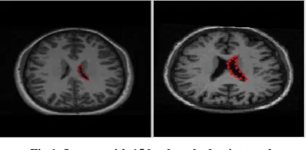
[image:2.595.317.538.290.398.2]

Good choices are clear corners of object boundaries, „T‟ junctions between boundaries or easily located biological landmarks[13]. However, it is not always the case that all images have enough clear corners, or easily located biological landmarks to describe the shape in its entirety. To get points that describe the shape entirely, the cornersand „T‟ junctions would have to be augmented with other points along boundaries which are arranged to be equally spaced between well-defined points.

Fig 1: Images with 15 landmarked points each.

3.2 Aligning the Training Set

The aim of this step is to align each shape so that the sum of distances of each shape to the mean is minimized. Given two similar shapes 𝐱𝑖and 𝐱𝑗, to align the latter with the former, we choose a rotation, 𝜃𝑗, a scaling, 𝑠𝑗, and a translation, (𝑡𝑥𝑗, 𝑡𝑦𝑗)

which maps 𝐱𝑖 onto M(𝑠𝑗, 𝜃𝑗)[𝐱𝑗] + 𝑡𝑗 so as to minimize the

weighted sum

𝐸𝑗= 𝐱𝑖− 𝐌 𝑠𝑗, 𝜃𝑗 𝐱𝑗 − 𝑡𝑗 𝑇𝑾(𝐱𝑖− 𝐌 𝑠𝑗, 𝜃𝑗 𝐱𝑗 − 𝑡𝑗 ) (1)

Where W is a diagonal matrix of weights for each point and

𝑴 𝑠, 𝜃 𝑥_𝑦𝑗𝑘_𝑗𝑘 = 𝑠 𝑐𝑜𝑠𝜃 𝑥_{𝑠 𝑠𝑖𝑛𝜃 𝑥}𝑗𝑘− (𝑠 𝑠𝑖𝑛𝜃)𝑦𝑗𝑘

𝑗𝑘 + (𝑠 𝑐𝑜𝑠𝜃)𝑦𝑗𝑘 , (2)

The alignment process removes differences due to translation, rotation and scaling.The alignment algorithm is as follows:

 Translate each shape instance so that its centre of mass is at the origin

 Align every shape in the training set with the first shape (or any other shape) in the training set by rotating, scaling and translating

REPEAT UNTIL CONVERGENCE

 Calculate the mean from the aligned shapes

 Normalize the orientation, scale and origin of the mean  Re-align every shape with the current mean

(3)

[image:3.595.53.222.118.258.2]

chosen that minimizes

(𝐷 = 𝑥

_𝑖

− 𝑥

2

)

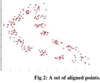
. The scale constraint means that all the corners lie on a circle about the origin.

Fig 2: A set of aligned points.

3.3 Modeling Shape Variation

At this point, we now have a set of points which are aligned into a common co-ordinate frame. Our aim is to build a model from which we can generate shapes similar to those in the training set. First, we have to reduce the dimensionality of the data from n-dimension to something smaller using Principal Component Analysis. The data form a cloud of points in the n-dimensional space. PCA computes the main axes of this cloud, allowing one to approximate any of the original points using a model with fewer than n parameters. Modeling shape variation is as follows:

Compute the mean of the data,

𝑥 = _𝑚1 𝑚𝑖=1𝑥𝑖 (3)

Compute the covariance of the data,

𝑺 = _𝑚−11 𝑚𝑖=1 𝑥𝑖− 𝑥 𝑥𝑖− 𝑥 𝑇 (4)

Compute the eigenvectors, 𝑝𝑖 and the corresponding t

eigenvalues 𝜆𝑖 of 𝑺 (sorted).

Any point in our allowable shape domain can be reached by taking the mean and adding a linear combination of the eigenvectors. Any shape in the training set can be approximated using the mean shape and a weighted sum of these deviations t modes:

𝐱 = 𝐱 + 𝐏𝐛,(5)

Where P = (𝐩1𝐩2… . 𝐩𝑡)is the matrix of the first t

eigenvectors and b = (b1b2… b𝑡)𝑇 is a t dimensional vector of

weights given by

b = 𝐏𝑻_{(x − x ) (6)}

The vector b defines a set of parameters of a deformable model and by varying its values within suitable limits, we can generate new examples of plausible shapes. The limits for the values of the vector b are derived by examining the distributions of the parameter values required to generate the training set. Suitable limits for b𝑘 are of the order

−3 𝜆𝑘≤ 𝑏𝑘 ≤ 3 𝜆𝑘 (7)

Alternatively, {𝑏1… … . 𝑏𝑡} can be chosen such that the

Mahalanobis distance 𝐷𝑚 from the mean is less than a

suitable value, 𝐷𝑚𝑎𝑥:

𝐷𝑚2 = 𝑏𝑘

2

𝜆𝑘

𝑡

𝑘=1 ≤ 𝐷𝑚𝑎𝑥2 (8)

The number of modes t can be chosen in one of several ways. The simplest way is probably to choose t that accounts for agiven proportion (e.g. 98%) of the variance exhibited in the training data.

3.4 Using Shape Models in Image Search

Having generated a Point Distribution model, we would like to use this model in image search. We must then find the set of parameters which best match the model to the image. Given a rough starting approximation, a model instance can be fit to an image. For each point in the rough starting approximation, it searches for better points around that point, usually along the normal. The initial approximation takes the form of estimates for the position at which the model should be placed, its orientation, scale and shape parameters required to fit the model to the image. After the initialization, we now wish to find the bestpose and shape parameters to match a model instance to a new set of image points Y.

An iterative approach for achieving this is as follows:

Initialize the shape parameters, b, to zero

REPEAT UNTIL CONVERGED

Generate the model instance 𝐱 = 𝐱 + 𝐏𝐛

Find the pose parameters (𝑋𝑡, 𝑌𝑡, 𝑠, 𝜃) which best maps x to

the new points Y.

Invert the pose parameters and use to project Y into the model co-ordinate frame:

𝑦 = 𝑇𝑋𝑡,𝑌𝑡,𝑠,𝜃

−1 _{(𝑌) (9)}

Project y into the tangent plane to 𝐱 by scaling 1/(y.𝐱 ).

Update model parameters to match y

𝐛 = 𝐏𝑇_{(𝑦 − 𝐱 )(10)}

Apply constraints on b.

3.5 K-NEAREST NEIGHBOUR

In this section, the K-nearest neighbor algorithm is described briefly for the purpose of an unfamiliar reader. KNN is a non-parametric (does not make assumptions about the distribution of the data) learning algorithm. It does not use training data points for generalization, rather on receipt of a new data instance, it computes the instance‟s K nearest neighbours from the dataset and makes a decision based on those.

To perform a KNN classification, we represent our dataset X

as an MxN matrix with M training examples with each example consisting of N features and a vector Y of length M representing output values for each training example.

Given a query input q, KNN can classify q with the following steps.

For each instance in the dataset

Compute the distance (say Euclidean) between q and datapoint𝐗𝒊 in dataset

Select K closest neighbours

Calculate majority.

(4)

4. KNN-ACTIVE SHAPE MODEL

[image:4.595.321.538.199.271.2]

In this section,the proposed KNN-ASM is presented. The proposed model describes a new way of moving landmark points to better positions after ASM image search. Haar filters are used to extract local imageedge features and K-Nearest Neighbour algorithm is used to learn better positions for each landmark. The best position is the position whose local edge structure is closest to a corresponding landmark. First, points are marked manually and those points are used to create a point distribution model as described in the preceding section. The model is then used to search for an object of interest in a new image as in the original ASM. The KNN-ASM then examines a small grid around each point for better points.

Fig 3: Positive and Negative examples.

[image:4.595.55.207.222.307.2]

Haar features can encode ad-hoc domain knowledge that is difficult to learn using a finite quantity of training data. Haar features are extracted from points as described in [9] by first creating an integral image and then extracting features from the integral image.

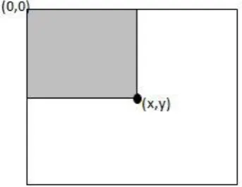
Fig 4: The value of integral image at point 𝒙, 𝒚 is the sum of all pixels from (0,0) to (x,y).

The integral image helps to compute haar features very rapidly.The integral image is computed in one pass over the image using the recurrence

𝑠 𝑥, 𝑦 = 𝑠 𝑥, 𝑦 − 1 + 𝑖 𝑥, 𝑦 (11) 𝑖𝑖 𝑥, 𝑦 = 𝑖𝑖 𝑥 − 1, 𝑦 + 𝑠 𝑥, 𝑦 (12) Where 𝑠 𝑥, 𝑦 is the cumulative row sum,𝑠 𝑥, −1 = 0,

and 𝑖𝑖 −1, 𝑦 = 0.

[image:4.595.60.232.385.518.2]

After computing the integral image, haar filters are used to extract features from the integral image.

Fig 5: Haar-based rectangular features.

Positive examples are features extracted from manually marked points (points marked with blue in fig 3) and negative examples are nearby points (points marked with red in fig 3). Having a set of features𝑿 = {𝐱1, … … , 𝐱𝑚}𝑇with known labels𝒀 = {𝑦1, … … , 𝑦𝑚}𝑇 for every land mark point in the training images, any point in a new image can now be classified against its corresponding feature set as a good or bad point.

(5)

[image:5.595.81.546.93.351.2]

Fig 6: KNN-ASM Framework

5. EXPERIMENTS AND RESULTS

[image:5.595.314.538.377.647.2]

In this section, experiments carried out on axial 2d slices of T2 MRI brain images are presented. 86 images were marked up with 15 points each. These points were used to create a Point Distribution Model. Images to be tested are read and the model is initialized on the images using the template matching scheme. ASM search is performed to fit the model to the ventricle in the image. Below are some of the results of the ASM and KNN-ASM alongside their dice overlap values:

Fig 7:ASM result1(.87)Fig 8:KNN-ASM result1(.88)

Fig 9:ASM result2(.82) Fig 10:KNN-ASM result2(.84)

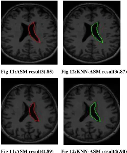
[image:5.595.51.260.481.729.2] [image:5.595.54.261.485.605.2]

[image:5.595.55.259.619.728.2]

A total of 23 images with available ground truth were tested and the segmentation accuracy of each was checked against their corresponding correctly segmented images using the dice overlap metric. The KNN-ASM achieved an improved segmentation accuracy on the average of 81.22% over the ASM‟s 80.37%.

(6)

6. CONCLUSION AND FUTURE WORK

In this paper, an algorithm which combines the popular Active Shape Model with a machine learning algorithm to improvethe segmentation accuracy of medical images has been proposed. In the proposed algorithm, final points that resulted from the ASM search are used as starting points for the KNN-ASM, with a small neighbourhood of each point being examined for better positions for the points. We validated the effectiveness of the proposed algorithm using a good number of images of the brain as we segmented the lateral ventricles of the brain. Results show that machine learning techniques can significantly improve the performance of Active Shape Model in medical image segmentation in the way described in this paper.

For future work, I propose the exploration of other machine learning algorithms like random forest and also the extension of this idea to segmenting other medical images apart from brain images.

7. ACKNOWLEDGMENTS

My thanks to Dr. Kola Babalola who provided me with the images that were used in this work.

8. REFERENCES

[1]. D. Cristinacce and T.F. Cootes, "Boosted Regression Active Shape Models", Proc. British Machine Vision Conference, Vol. 2, 2007, pp.880-889.

[2]. Etyngier P, Ségonne F, Keriven R, “Active-contour-based image segmentation using machine learning techniques”. Med Image Comput Assist Interv. 2007;10(Pt 1):891-9.

[3]. Jain V, Seung HS, Turaga SC, “Machines that learn to segment images: a crucial technology for connectomics”.CurrOpinNeurobiol. 2010 Oct;20(5):653-66.

[4]. L. Padma Suresh, K.L. Shunmuganathan and S.H. Krishna Veni, “Dermoscopic Image Segmentation using Machine Learning Algorithm”, American Journal of Applied Sciences 8 (11): 1159-1168, 2011.

[5]. Neeraj Sharma and Laht M. Aggarwal, “Automatic medical image segmentation techniques”. Journal of medical physics. Jmedphys 2010, Jan-Mar, 35(1) 3-14.

[6]. Nils Plath, Marc Toussaint, Shinichi Nakajima, “Multi-class image segmentation using conditional random fields and global classification”. Proceedings of the 26th Annual International Conference on Machine Learning, 2009,pp.817-824.

[7]. P. Etyngier , F. Segonne and R. Keriven N. Ayache , S. Ourselin and A. Maeder "Active-Contour-Based Image Segmentation Using Machine Learning Techniques", Proc. Medical Image Computing and Computer-Assisted Intervention, pp.891 -899 2007.

[8]. P. Viola and M. Jones. “Robust real-time object detection”. International Journal of Computer Vision, 57(2):137_154, 2004.

[9]. Salem Almari, N.V. Kalyankar and Khamitkar S.D, “Image segmentation by using Thresholding techniques”. Journal of Computing, vol 2, issue 5, May 2010, ISSN 2151-9617.

[10].Shuyu Li, Litao Zhu, Tianzi Jiang, “Active Shape Model Segmentation Using Local Edge Structures and AdaBoost”. Medical Imaging and Augmented Reality Lecture Notes in Computer Science Volume 3150, 2004, pp 121-128.

[11].Srinivas C. Turaga, Kevin L. Briggman, Moritz Helmstaedter, Winfried Denk, H. Sebastian Seung, “Maximin affinity learning of image segmentation”, In Advances in Neural Information Processing Systems 22 (2009), pp. 1865-1873.

[12].T.F. Cootes, D. Cooper, C.J. Taylor and J. Graham, "Active Shape Models - Their Training and Application." Computer Vision and Image Understanding. Vol. 61, No. 1, Jan. 1995, pp. 38-59.

[13].T.F.Cootes, G.J. Edwards and C.J.Taylor. "Active Appearance Models", IEEE PAMI, Vol.23, No.6, pp.681-685, 2001.