An Evolutionary Approach for Solving the N Jobs M Machines Permutation Flow Shop Scheduling Problem with Break Down Times

(1)

An Evolutionary Approach for Solving the N-Jobs

M-Machines Permutation Flow-Shop Scheduling Problem

with Break-Down Times

Armando

Rosas-González

Technological University of the Mixteca

Road to Acatlima Km. 2.5 Huajuapan de León, Oaxaca,

México, 69000

Dulce-María

Clemente-Guerrero

México, 69000

Jorge-Carmen

Flores-Juan

México, 69000

Santiago-Omar

Caballero-Morales

México, 69000

ABSTRACT

In this paper a Genetic Algorithm (GA) approach is presented to solve the N-Jobs M-Machines Permutation Flow-Shop Scheduling Problem (PFSP) with Break-down times. In comparison with other methods that start with a solution obtained with the Johnson’s Algorithm (or another greedy approach), the presented GA method starts with randomly generated solutions and within 100 iterations is able to obtain a solution better than other methods. Also, while in other works the sequence of jobs to be processed in the machines is obtained prior to the occurrence of break-down times, the GA finds the solution considering from the beginning the occurrence of the break-down times. Thus, the presented GA method considers the effect of the break-down times in the overall process. A selection of standard 20×20 PFSPs was used for validation of the GA, finding that in 86% of the selected PFSPs the GA was able to provide job sequences with better makespans when compared with another method. The makespan improvements were statistically significant at the 0.10 and 0.01 levels. Then, evaluation of the GA was performed on one PFSP case with break-down times. As in the validation cases with standard PFSPs, the GA outperformed the results obtained with another method.

General Terms

Industrial Engineering, Permutation Flow-Shop Scheduling Problem.

Keywords

Flow-Shop Scheduling, Break-Down Times, Genetic Algorithms.

1. INTRODUCTION

Flow-shop is one of the main scheduling problems in manufacturing [1]. Flow-shop scheduling is used to determine the optimal sequence of N-jobs to be processed on M-machines in the same order [2]. In the permutation flow-shop scheduling problem (PFSP) the same sequence of jobs must

be performed on all machines, one machine can only process one job at a time, and no machine is allowed to be re-visited [3]. The optimal sequence of jobs is the one that minimizes the makespan of the N-jobs through the M-machines, this is, the minimization of the completion time of the last job on the last machine [2, 4].

Three main factors are known to be related to scheduling problems: job transportation time (which includes moving and idle times), relative importance of a job over another, and break-down time of machines [5]. Break-down times represent the periods or time intervals where processing may be stopped due to interruption of energy or raw material supply, failures, or due to maintenance tasks [6]. Flow-shop scheduling with break-down times has been studied as presented in [5, 6] with diverse conditions and solving methods. For example, in [7] an optimal sequence was obtained for the 2-machines N-jobs flow-shop with random break-down times. In [6] a heuristic approach was proposed for solving the 3-machines N-jobs flow-shop considering transportation times and weights of jobs in addition to break-down times. In [8] the makespan for a flexible flow-shop was optimized by using a decomposition based algorithm (DBA). Another work involving a 3-machines N-jobs flow-shop was presented in [9] where a heuristic algorithm was proposed for solving the scheduling problem with break-down times and weights of jobs. Finally, in [10] a branch-and-bound algorithm was presented to solve the 3-machines N-jobs flow-shop scheduling problem with break-down and transportation times. Note that many of the works available consider the case with a limited number of machines (e.g., M=2, 3).

(2)

International Journal of Computer Applications (0975 – 8887) Volume 83 – No1, December 2013

sizes up to N=M=20. The improvements obtained in makespan were statistically significant.

The present work is structured as follows: in Section 2 an overview of the PFSP with break-down times is presented. Then in Section 3 the details of the GA approach for solving the PFSP with breakdown times and N-jobs M-machines is presented. In Section 4 the results of the GA approach on case studies are discussed. Finally, in Section 5 the conclusions and future work are presented.

2. PFSP WITH BREAK-DOWN TIMES

The PFSP with break-down times with N-jobs and M-machines is defined as follows:

o All N-jobs are processed through M processing centers P1,

P2, ..., PM in the same order (e.g., each job is processed

first in center P1, then P2, ..., until PM).

o i represents the job in an arbitrary sequence, where i = 1,...,N.

o All N-jobs are available to be processed at time zero.

o Pi1, Pi2, Pi3, ..., PiM, represents the processing time of job i

in the processing center P1, P2, P3, ..., PM respectively.

o The break-down interval is defined as (a, b), and the interval length is (b - a).

o If break-down conditions take place and interruption of power supply occurs, the processing times of the centers may be affected accordingly to the type of center. These can be classified under three categories:

 U: Processes that cannot be interrupted. In this case, breakdown time is applied and the process itself is postponed. This is common for processes as moulding, casting, forging, and welding [5]. The processing time in this case is modified and (b - s1) is

added to the original processing time.

 V: Processes that require power supply and, if break-down occurs between the process (which starts at time s1and ends at time s2), can be resumed when power

supply returns. Processes that can be classified in this category are packing, machining, threading, and drilling [5]. In this case, original processing times are modified as follows:

 if break-down starts between s1 and s2, (b - a) is

added to the original processing time;

 if break-down starts and ends between s1 and s2, (b

- a) is added to the original processing time;  if break-down ends between s1 and s2, (b - s1) is

added to the original processing time;

 if break-down starts before s1 and ends after s2, (b

- s1) is added to the original processing time.

 W: Processes that do not require power supply can continue during the break-down time. Thus, no modification in the original processing time is required.

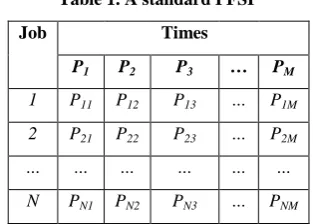
[image:2.595.349.506.78.190.2]

The information of a PFSP is commonly presented as shown in Table 1. Other works also consider weights for the jobs in order to represent their importance in the process sequence [6, 9] however the present work is focused on the solving method for N-jobs and M-machines.

Table 1. A standard PFSP

Job Times

P1 P2 P3 … PM

1 P11 P12 P13 … P1M

2 P21 P22 P23 … P2M

… … … … … …

N PN1 PN2 PN3 … PNM

3. THE GA METHOD

The PFSP has been solved with different methods. For example, in [11] a greedy heuristic was used while in [8] and [10] DBA and B&B (branch and bound) algorithms were used respectively. The use of a GA (Genetic Algorithm) was explored in [12] with significant results. For the PFSP with break-down times greedy heuristics have been applied [5], however the use of GAs has been limited.

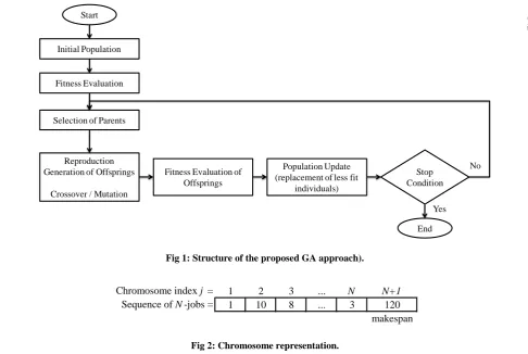
GAs are heuristics based on the natural process of evolution [13, 14]. These have been used to solve other combinatorial problems as the Travelling Salesman Problem (TSP) and Job-shop scheduling [15]. In this paper a GA is presented for the PFSP with break-down times with N-jobs and M-machines. In Figure 1 the general structure of the GA is shown and the details of each module are explained in the next sections.

3.1 Initial Population and Fitness

Evaluation

The initial population is the set of initial solutions for the PFSP. These can be randomly generated or be given by a fast heuristic algorithm [13]. These solutions are represented as “chromosomes” to enable diversification by means of the reproduction operators (crossover, mutation). In Figure 2 the chromosome representation of a solution for the PFSP is presented. The chromosome is a vector with N + 1 cells, where in the first N cells the sequence with N-jobs is stored and in the cell N +1 the makespan obtained through M-machines with that sequence is stored.

For this work a random initial population of X=1000 individuals was considered. Initially small initial populations (e.g., with size < 50 individuals) were considered as discussed in [16, 17]. However it was found that for the PFSP the reproduction operators were not able to efficiently diversify the solutions within small populations.

In a GA is important to measure the ability to solve a problem with an optimality criterion, or fitness, of each solution in the initial population. In this case, the optimality criterion consists in finding the solution with the minimum makespan, thus, the fitness is measured based on this concept. The makespan is the completion time of the last job on the last machine [2, 4].

3.2 Selection of Parents

(3)

In the PFSP, fitness is measured based on the makespan, and the “Roulette Wheel” selection method is one of the most used methods for selection of the fittest individuals without excluding less fitted individuals [18]. In the “Roulette Wheel” method, all chromosomes (individuals) are located into a roulette wheel in function of their fitness values. A segment of the roulette wheel is assigned to each individual based on its overall fitness with respect to the other individuals. Thus, the size of the segment is proportional to the individual’s fitness (e.g., largest segment = highest fitness). Then, when the roulette wheel is rotated the individuals with better fitness are more likely to be selected for reproduction, although there is also the possibility to select individuals with less fitness. This may be beneficial for the diversification process [19]. The steps of the roulette wheel selection for i = 1, …, n individuals are presented as follows [20]:

(1)Compute the fitness value ( ) for each i-chromosome in the population.

(2)Compute the sum of fitness ( ) for all chromosomes in the population:

(3)Compute the average fitness ( ) in the population:

(4)Compute the expected fitness ( ) for each chromosome in the population:

(5)Compute the sum of all expected fitness ( ) for the chromosomes in the population:

(6)Generate a random number ( ) within the range (0, ). (7)Select the chromosome for which the cumulative fitness

>=

(8)Go to step 6 and repeat n times.

3.3 Reproduction and Population Update

In order to diversify the initial solutions (generate new solutions) reproduction operators are used that work at the chromosome level of the individuals in a population (e.g., see

Figure 2). To generate “offspring” solutions, pairs of “parent” solutions are required. The first operator to be used in this work is the crossover operator which consists in the exchange of genes between “parent” chromosomes [13]. When the individuals consist of sequences where order is important (as is the case of the PFSP) the Partially Mapped Crossover (PMX) is the most suitable. In general, two offspring solutions are obtained from each pair of parent solutions using the PMX operator. Details of this operator can be found in [21].

The second operator is the mutation operator, and this consists in changing, randomly or deterministically, the element(s) in a chromosome [13]. In this case, offspring solutions were obtained by the exchange of two randomly selected genes in a chromosome. In general, one offspring is obtained from a single parent solution.

The number of offspring solutions obtained by using the crossover and mutation operators usually depends of a probability. In this case, the following probabilities were considered for crossover and mutation: PPMX and PMUT. By

considering X as the number of individuals in the population, the number of offspring solutions generated by crossover and mutation is defined as XPMX = X×PPMX and XMUT = X×PMUT,

where PPMX = 0.80 and PMUT = 0.30 were considered.

After all offspring solutions are generated (XPMX+XPMX) their

[image:3.595.53.540.28.354.2]

fitness is evaluated (e.g., the makespan is obtained for each offspring). When this is achieved, the initial population is updated, and the offspring solutions with better fitness replace the original parents with worse fitness. At the end, and updated population with X individuals is obtained, which consists of parents and offsprings. These individuals will be the new parents for new offsprings by repeating the same process of selection and reproduction, thus generating a new population. This updating process is iterated and repeated Fig 1: Structure of the proposed GA approach).

Fig 2: Chromosome representation.

Initial Population

Fitness Evaluation

Selection of Parents

Reproduction Generation of Offsprings

Crossover / Mutation

Fitness Evaluation of Offsprings

Population Update (replacement of less fit

individuals)

Stop Condition

End Yes

No

Chromosome index j = 1 2 3 ... N N+1

Sequence of N-jobs = 1 10 8 ... 3 120

(4)

until a stop condition is met. This is explained in the following section.

3.4 Stop Condition

As commented, the new population is considered the initial population for the next iteration (generation) of the GA. The process of selection, reproduction, and update, is repeated until a stop condition is met, however there is no overall condition to stop the GA. While a common practice is to stop the GA when there are no change in the population’s average fitness (convergence is achieved), other practices involve considering a fixed number of iterations. In this case a total of T = 200 iterations (generations) was considered.

4. EXPERIMENTS

The GA approach was tested with two types of case studies. The first consisted of the standard PFSP (no break-down times). This was considered important to evaluate and validate the performance of the GA for large problems (in this case, with N=M=20). Then, the second type consisted of the PFSP with break-down times. The results are presented in the following sections.

4.1 Standard PFSP

For the validation of the GA the PFSP problems defined in [22] were considered. Particularly, the PFSPs with size 20×20 (N=M=20) were considered as the instances in [22] provided two important values for comparison: Lower Bound (LB) and Best Known Solution (BEST). In this case, a population of 1000 was used for the GA given the size of the PFSP. In Table 2 the makespan results obtained with the GA and the method used in [22] (BEST) for 28 randomly selected 20×20 PFSPs are presented.

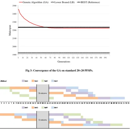
As presented in Table 2, in 24 out of the 28 PFSPs a solution that led to a better makespan was found with the GA in comparison with the results reported in [22] for the same PFSPs. This is an improvement in 86% of the PFSPs and the convergence of the GA is also presented. In Figure 3 the convergence plot of the GA across all PFSPs is presented. The overall makespan across al PFSPs starts at iteration 0 with 2450 approximately, however, as the diversification (reproduction) is performed the individuals in the population become more fit and thus, overall makespan tends to decrease. At iteration 60 the overall fitness equals the fitness obtained with the method presented in [22] and after that iteration the individuals found with the GA are of better fitness. A pairs-match test was performed to evaluate the statistical significance of these results, obtaining a p-value of 1.44226E-05. Thus, the improvements are statistically significant at the 0.10 and 0.01 levels and there is confidence about the use of the GA for other PFSPs (including the case with break-down times).

Table 2. GA performance on standard 20×20 PFSPs

Problem LB BEST GA

1 1957 2213 2190

2 1854 2155 2121

3 2016 2307 2295

4 1825 2142 2152

11 1984 2299 2289

12 1922 2188 2193

15 1905 2272 2270

17 2044 2281 2273

23 2031 2259 2231

24 2017 2264 2259

29 1845 2119 2126

31 1846 2291 2274

32 1914 2289 2235

33 1859 2205 2192

42 1952 2337 2332

45 1906 2278 2273

50 1918 2308 2302

53 1898 2193 2203

56 1881 2211 2206

63 1853 2150 2146

66 1932 2197 2179

67 1894 2354 2351

70 1990 2323 2302

72 1861 2188 2178

77 1756 2121 2116

85 2125 2220 2189

89 1809 2182 2165

94 1993 2221 2201

4.2 Standard PFSP

The GA approach was tested with the following PFSP with breakdown times: 4-jobs 5-machines with known makespan = 53 [5]. In this work the processing centers 1 and 5 are catalogued as of “V” type while the processing center 2 is catalogued as type “M” and 3 and 4 as type “U”. A heuristic method was used to obtain the sequence that led to a makespan of 53. This sequence was obtained prior to adjust the processing times with the break-down times. After 3 iterations of the GA with an initial randomly generated population of 10 individuals a sequence with a makespan of 52 was obtained (which is lower than the baseline of 53). In Figure 4 the Gantt diagrams for both sequences are presented.

5. CONCLUSIONS AND FUTURE

WORK

In this work a GA approach was presented for solving the PFSPs with and without break-down times. Given the limited availability of numerical examples with break-down times we were only able to test the GA with a 4×5 PFSP. However, numerical examples with standard 20×20 PFSPs were found and improvements in 86% of cases were achieved. These improvements were statistically significant and thus there is confidence about the overall performance of the presented GA.

[image:4.595.344.515.71.333.2]

(5)

6. REFERENCES

[1] Gupta, D., Sharma, S., and Sharma, S. 2011. Heuristic Approach for n-Jobs, 3-Machines Flow Shop Scheduling Problem, Processing Time Associated With Probabilities Involving Transportation Time, Break-Down Interval, Weightage of Jobs and Job Block Criteria. Mathematical Theory and Modeling. 1(1), 30–36.

[2] Singhal, E., Singh, S., and Dayma, A. 2012. An Improved Heuristic for Permutation Flow Shop Scheduling (NEH ALGORITHM). International Journal of Computational Engineering Research. 2(6), 30–36. [3] Emmons, H. and Vairaktarakis, G. 2013. Flow Shop

Scheduling: Theoretical Results, Algorithms, and Applications. International Series in Operations Research & Management Science, Springer, New York.

[4] Baskar, N., Balasundaram, N., and Siva, R. 2012. A New Approach to Generate Dispatching Rules for Two Machine Flow Shop Scheduling Using Data Mining. In

Proc. of the International Conference on Modeling, Optimization and Computing (ICMOC2012), 238–245. [5] Baskar, A. and Xavior, A. 2012. A Simple Model to

Optimize General Flow-Shop Scheduling Problems with Known Break Down Time and Weights of Jobs. In Proc. of the International Conference on Modeling, Optimization and Computing (ICMOC 2012), 191–196. [6] Chandramouli, A. B. 2005. Heuristic Approach for

n-Job, 3-Machine Flow Shop Scheduling Problem Involving Transportation Time, Break Down Time and Weights of Jobs. Mathematical and Computational Applications. 10(2), 301–305.

[7] Allahverdi, A. and Mittenthal, J. 1994. Two-machine ordered flowshop scheduling under random break-downs. Mathl. Comput. Modelling. 20(2), 9–17. [8] Wang, K. and Choi, S. H. 2009. A decomposition based

[image:5.595.106.535.80.495.2]

algorithm for flexible flowshop scheduling with machine breakdown. In The IEEE International Conference on Fig 3: Convergence of the GA on standard 20×20 PFSPs.

Fig 4: Performance of the GA on a 4×5 PFSP with break-down times. 1900

2000 2100 2200 2300 2400 2500

1 11 21 31 41 51 61 71 81 91 101 111 121 131 141 151 161 171 181 191

M

ak

es

p

an

Generations

(6)

Computational Intelligence for Measurement Systems and Applications (CIMSA 2009). 134-139.

[9] Khodadadi, A. 2012. Solving Weighted Flow-Shop Scheduling Problem Involving Break-Down Time of Jobs for Machines. Journal of International Academic Research. 12(1), 10–15.

[10] Gupta, D. 2012. Branch and Bound Technique for three stage Flow Shop Scheduling Problem Including Breakdown Interval and Transportation Time. Journal of Information Engineering and Applications. 2(1), 24–29. [11] Finke, G. and Jiang, H. 1997. A variant of the

permutation flowshop model with variable processing times. Discrete Applied Mathematics. 76, 123–140. [12] Akhshabi, M., Haddadnia, J., and Akhshabi, M. 2012.

Solving flow-shop scheduling problem using a parallel genetic algorithm. Procedia Technology. 1, 351–355. [13] Goldberg, D. E. 1989. Genetic Algorithms: in Search,

Optimization and Machine Learning. Addison Wesley, Massachusetts.

[14] Cerrolaza, M. and Annicchiarico, W. 1996. Algoritmos de optimización estructural basados en simulación genética. U. C. V.-Consejo de Desarrollo Científico y Humanístico, Caracas.

[15] Chan, F. and Choy, K.L. 2011. A genetic algorithm-based scheduler for multiproduct parallel machine sheet metal job shop. Expert systems with Applications. 38, 8703–8715.

[16] Martín, E. and Valeiras, G. 2004. Sistemas Evolutivos y Selección de Indicadores. Universidad de Sevilla-Secretariado de Publicaciones, Sevilla.

[17] Alander, J.T. 1992. On optimal population size of genetic algorithms. In Proc. of the 6th Annual European Computer Conference.

[18] Escolano, F., Cazorla, M. A., Alfonso, M. I., Colomina, O., and Lozano, M. A. 2003. Inteligencia Artificial: Modelos, Técnicas y Áreas de Aplicación. Thomson Ediciones, Madrid.

[19] Kumar, R. 2012. Blending roulette wheel selection & rank selection in genetic algorithms. International Journal of Machine Learning and Computing. 2(4), 365-370.

[20] Firas, A. and Reyadh, N. 2012. Comparison of Selection Methods and Crossover Operations using Steady State Genetic Based Intrusion Detection System. Journal of Emerging Trends in Computing and Information Sciences. 3(7), 1053-1058.

[21] Deep, K. and Mebrahtu, H. 2012. Variant of partially mapped crossover for the Travelling Salesman problems. International Journal of Combinatorial Optimization Problems and Informatics. 3(1), 47–69.