Posterior Analysis of Sequential Normal Testing Procedure

Posterior Analysis of Sequential Normal Testing

Procedure

Birjesh kumar

J.P Institute of Engg &Technology,Meerut A-115 ganga sagar colony

Ganganagar,Meerut

Abha Chandra,

PhD Deptt.of Statistics Meerut college,Meerut

K.K.Sharma,

PhD Retd Prof&Head Deptt.of Statistics C.C.S University,Meerut

ABSTRACT

Several studies deals with the non- robust character of various types of acceptance plans. Many such studies also analyze the robust character of sequential testing procedures when the underlying failure time distribution has a monotone failure rate. A vast literature on the life testing plans in the Bayesian framework is also available where updating prior with experimental data has been the main concern. Highlighting the point that the basic normal lifetime distribution can also be updated in respect of prior variations in the involve parameters. The present study deals with the analysis of the robust character of sequential normal testing procedures when the mean of the basic normal distribution is considered as a random variable. The robust character of the consistency of the random variable n, in view of prior variations, is also analyzed

Keywords

Robustness, SNTP, OC, ASN and Coefficient of variation function(C.V).

1.

INTRODUCTION

An important contribution in the area of sequential test of statistical hypothesis is due to A. Wald (1947), who developed sequential probability ratio test (SPRT) for testing a simple hypothesis against a simple alternative. He obtained the expressions for operating characteristic (O.C.) and average sample numbers (ASN) function of the SPRT. The robustness of the SPRT, when the distribution under consideration has undergone a change, has been studied by various authors while dealing with various probability models, like Montagne and Singapurwala (1985), Sharma K.K. and Rana (1990), Sharma K.K. and Bhutani (1992) and others. The robustness of these procedures has been investigated in respect of producer's and consumer's risk and the ASN.

Further on using different life time models, the studies in [2A] include a vast literature on the life testing plans in Bayesian framework in which updating the prior with experimental data has been the main concern. However, in the Bayesian framework, it should be recognized that priors do have an impact on the basic distribution and therefore the basic distribution can be updated in view of prior variations. This updated basic distribution be used in the analysis. In the present paper we consider SPRT for testing the

0

:

H

 



_

v/s

H

1

:

 



1 _{when samples are} sequentially recorded from





2

,

N

 







being known. Further, when we consider  to be a random variable we use

the prior of  to update the basic distribution

,

N



 







and use this basic updated distribution to study the robust character of SPRT when  is considered to be a random variable. The concept has been highlighted in the present study.

Further, it was also noted that the basic distribution can be further updated in respect of the posterior distribution. This further updated distribution is also named as predictive basic distribution.

In view of above, the present paper considers the robust character of SPRT, when predictive distribution is used in the analysis. A comparison of OC , ASN curve and C.V curve in the corresponding situation has been used as the basis of analysis.

2.

NOTATIONS

N(, 2) : Normal distribution with mean  and variance 2

p.d.f. : Probability density function

SPRT : Sequential probability ratio test

SNTP : Sequential normal testing procedure L() : The OC function, the probability of

accepting H0 when  is the true parametric value

n : The sample size needed to terminate the sequential testing. Thus n is a random variable.

E(n) : ASN functions for fixed .

V



(n)

:

Variance of the random variable n for fixed 

CV(n)

_:

Co-efficient of variation of the random variable n for fixed 

 : Size of the type I error, also called producer's risk in quality control terminology.



MTSF

:

;

Size of the type II error, also called consumer's risk in quality control terminology.

Mean Time to system failure

3.

STATISTICAL BACKGROUND

For developing the procedure we assume that (i)The failure

time distribution of X is





2 1

N

 







2 1 1 2 2 1 1 1

1

,

;

,

0

2

x

f

x

e

x





 







       _{ } 





   



...(1) Here , µ is the MTSF and σ1 is assumed known.

(ii) The lot to lot quality,  is a random variable having its known conjugate prior distribution as normal with p.d.f.





2 2 1 2 2 2 2 2

1

;

,

0

2

g

e

 



  









        

 



   



...(2)

(iii) Further let x



x1,x2,...,xn



 be random

sample of size n from the population in (1) then the posterior distribution of  forgiven X~ will be

2 2 2 2

2 1 1 2

2 2 2 2

1 2 1 2

1 2 2 2 2 1 2 2 1 2

1

2

nx n n

n

e

x

        











 

 _   _     _{ } _       



 



 

 





2



N

x









 



_

_





_





……… (3)

where 2 2 2 2 2 1

nx

n











 







and 2

2 1 2

2 2 2 1

n

 













(iv) Finally, in view of (1) and (3) the predictive distribution of the future observations [8] that is the updated compound distribution of X can also be obtained

as

 



2







1

, ,

h x x



f x

 



x d



















2 2 2 1 1 2 2 2 1

1

2

x

e



 







 _      _   





;

 

   

3

,

h x x

N

 



f x

 















……….. (4) …(4)

Now here

E(X) =

2 2 2 1 2 2 2 1 nx n       _       

  _and

Var (X) =

2 2

1











_

_







Also the distribution of x in (4) is N



 







.The respective basic and predictive distributions in (1) and (4) enable us to analyse the robust character of SNTP with respect to α , β and Eµ (n) in the following situations

-

(1) The basic distribution in (1) is used in the analysis when µ is considered as a constant.

(2) The predictive basic distribution in (4) which is updated in respect of posterior distribution of µ is used in the analysis when µ is considered as a random variable. Obviously, this updated distribution also includes information on experimental data.

4. OC AND ASN FUNCTIONS FOR SNTP

WHEN



IS CONSIDERED AS A

CONSTANT

In this case, SNTP for testing the null hypothesis

0

:

H

 



_





_

v/s

H

1

:

 



1





 we assume that the sample observations are being sequentially recorded from the basic distribution in (1) i.e.





,

N

 



_



_

being known.

Here, following [13]. The approximations to the OC function of the present SNTP can be obtained by considering the

values of

g



g

 





0

which satisfy









1 1

1 0 1

, , 1 , , g f x E f x             

or













1 1 1

1 0 1

, ,

, 1

, ,

g

f x

f x dx f x   _{ }    _            



...(5)

On simplifying (5), one gets the following pair of parametric equations providing approximations to the OC function---









2

g   

            _   

  _and

 

g 1

g g A L A B



 _    _ 

  _……(6)

A plot of L

 

 against  provides us the OC curve. Here,

1 ,

A  B 

 



 

  _and











Further, the approximated formula for ASN of present SNTP will be

 

L

 

LogB



1

_{ }

L

 



LogA

   



 







  2 1 1 1 2 2

L LogB L LogA

E n

                     

…...(7)

Here

 

2









1

1

2 2

E z 

_









 

 





 

……..(8)

The notable features of the equation in (6) is that this is

independent of 2 1



_.

Thus, the OC curves for the present SNTP remains static with

variations in 2 1



_{. As a consequence the points}

 

, 1

 

  

  _and



1, 



_{on the OC curve also} remain static with variations in 12 _{as such. The present} SNTP is found to be robust in respect to '' and '' with

variation in 2 1



. On the other hand, the expression for

 

E

_

n

in (7) is a function of 2 1



_{. However, it seems}

logical that variation in 2 1



should obviously have an effect on the size of two errors, but the present SNTP is observed to be an exception in this regard. Still, the results in (6) and (7) provide us a basis for investigating the robustness of SNTP in respect of ,  and ASN when µ is considered as a random variable.

5. ROBUSTNESS OF THE PRESENT

SNTP

IN

RESPECT

OF

PRIOR

VARIATIONS WITH EXPERIMENTAL

DATA

Given a sequence of observation

x x

1

,

2

,...,

x

n from (1) Suppose one wishes to test the null hypothesis

0

:

H

 



_

=λ0v/s H1 :





1









  _=λ

1 ,In order

to study the robustness of the SPRT developed in section 4 in respect of OC and ASN function. We consider h1 as solution of the equation









1 3 3 0

,

,

1

,

,

h

f

x

E

f

x

 

 

 _ 





_



_











































1 3 3 3 0

,

,

, ,

1

,

,

h

f

x

f

x

dx

f

x

 

 

 

 _ 





















……….. (9)

it is notable that the expression in (9) is in respect of the predictive distribution in (3). The OC curve for testing

0

:

H

 



_





_

v/s

H

1

:

 



1





 is obtained approximately by the following pair of equations on solving (9), we get









2

'

h

 



 

   













_











_and

 

_'h'

1

_'

h h

A

L

A

B









…………. (10)

Thus a comparison of the OC curve in (5) and (10) help us in analyzing the robust character of SNTP in respect of  and  when updated prior has been used on using experimental data.

(3) Similarly, for analyzing the robustness of ASN function for SNTP we obtain

 

3

_



1



_

3 0

,

,

f

x

E

z

E Log

f

x



 



_{ }

 



_

























3 1 3 3 0 , , , f x

Log f x dx

f x

 

_{ }

 

      _ _    



 

1









2

2

E

_

z





 





      









_







_

……… (11)

Here, also the expectation is taken in respect of the predictive normal distribution on using (9) one easily gets,

 

 



 





2 2







0 1 1 0

1

og

1

2

2

L

LogB

L

L

A

E

_

n









  





 

















………(12)

For σ1 = β, Thus a comparison of the ASN in (7) and in (12) help us in analyzing the robust character of SNTP in respect of ASN when the prior can be updated in the form of posterior on using experimental data in Bayesian framework

6. ANALYZING THE ROBUSTNESS OF

THE CONSISTENCY OF N WHEN



IS

CONSIDERED

AS

A

RANDOM

VARIABLE.

Recognizing the fact that in all sequential testing procedures n is a random variable, as such, the ASN function,

i.e.,

E



 

n

alone cannot be taken as a measure of effectiveness of the testing procedure. In this regard,

 

V n

_

is a measure of the consistent behavior which can be analyzed by using a relative measure of dispersion, called the co-efficient of variation (C.V.) the C.V. in the present case will be

 

.

C V

_

n

 

 

100

V n E n     ……….. .(13)

For developing formula for C V. 

 

n _{we proceed to}

Following the assumptions as used in the derivation of

 

E n

_

by Wald (1947), we consider



Z

1



Z

2



...

Z

N

 



Z

1



Z

2



...

Z

n

 



Z

n1



...

Z

N



Where









2 2 2 2 0 , , , , f x Z Log f x                 

Also for α > n, the random variable Z _{is distributed}

independently of n.

Thus



1 2

...

N

 

1 2

...

n

 

n1

...

N



V Z

 

Z

Z



V Z

 

Z

Z



V Z

_



Z

…………... (14)

Now, consider the term

1 1

N N

i i

i n i n

Z

V

Z

V

n

   







































1 1 N N i i

i n i n

Z Z

V E E V

n n             _ _  _ _       



 







  



  

V

N

n E z

E

N

n V z

 

_



  

_

_





_

 

2

 

  



E z

V n

V z E N

n

 

_



_





 

2

 

 

 

E z

V n

V z

N

E n

 

_



_



 

_



_

………... (15)

On using (14) in (13), One gets

 

2

 

   

1

0

n

i i

V

Z

E z

V n

V z E n







 









_{ }

_











or

 

   

 

1 2 n i i

V z E n V Z

V n E z     _ _       



Since all the terms in V n

 

are function of , thus the above can be re-written as

 

 

 

 

1 2 n i i

V z E n V Z

V n E z          _ _       



……… (16)

6(a)

C V n

.

_

 

When



is Constant

In this case, the expression for

E



 

n

and

E



 

z

are as given in (7) and (8) respectively, further, it is easy to obtain

 

 

₂

 

2

V

_

z



E

_

z

 



E

_

z



_





2 2 1

 











………….... (17) and

 

 





2

1

1

n i i

V Z L



L



LogB LogA

          _{ }   





………... ………… (18)

On using (7), (8) (17) and (18) in (16), one gets V

 

n in the present case and therefore,

 

V

_{ }

 

n 100

CV n E n      ………... (19)

6 (b)

C V

. .

_

 

n

when



is random variable

In this case, the expression for E

 

n and

E



 

z

are as given in (12) and (11) respectively, further one easily gets

 

 

₂

 

2





2

V

_

z

E

_

z

E

_

z

 



  





 

_

 

_

………..………... (20) and

 

  



2

1

1

n

i i

V

z

L



L



LogB

LogA









 









_

_











………..(21)

On using (11), (12), (20) and (21) in (16) one easily

get V

 

n and consequently

 

_{ }

 

. V n 100

C V n

E n      ………... (22)

Now, the trend in C V. 

 

n and C V. 

 

n for varying  and  can be used to study the robust character of the consistency of the random variable n, when  is random variable.

7. DISCUSSION

study the robust characters of SNTP in respect of ,  and ASN function when prior has been updated with posterior as its distribution. For meeting this objective, we compare the generalized form of OC. curve in (6) with its particular form given in (10). Similarly, the generalized form of ASN in (7) is compared with its particular form in (12) so the last

 

.

C V

_

n

and

C V

.



 

n

as given in (19) and (22) respectively are compared to analysis the robust character of the consistency of the random variable n when µ is considered as a random variable with posterior as its distribution. For clarity, we consider an example

8. An example

We have considered the SPRT for testing the hypothesis

0

:

50

H

  

  

_{ }

v/s

H

1

:

 









1



47

when observations are sequential recorded from



2



1

50, 64

N





and that for  in (2) will be



2



2

50, 36

N





,

further suppose that the process sample information

1, 2,... n

X X X _{yields X 53 for n = 25, Then on}

using (3) and (4), we have

2 2

2 1

2 2

1 2

52.80

nx

n



















2 2

1









 _{ } 

 

66.39





_

In other words, the predictive normal distribution of X

becomes

N



52.80, 66.39



. Now on using the expression in (6), (7) and (19), a few respective point on

 

L



,E

 

n and C V. 

 

n for varying  have been summarized in Table-1. Now on considering the predictive basic distribution of X in (4), the expression in (10), (12) and

(22) the respective points on L

 



,E

 

n and

  .

C V n _{have also been listed in Table-1. For still better}

analysis of the non- robust character of SNTP in respect of ,

 and ASN, when posterior prior has been used, the points in

Table-1 are used to draw the curves for

L

 



/

L

 



,

 

E

_

n

/

E



 

n

and C V. 

 

n /C V. 

 

n for varying





E

 







in figure 1, 2 and 3 respectively.

9. Analysis

According to A. Wald [1947], the basis of selecting a desirable sequential test involves the following steps.

1. We first consider admissible sequential test of the same

strength



 



.

2. Then from among the admissible test, A test provide

minimumE

 

n , for all values of  is considered as most desirable

.

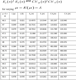
Table 1:

Showing values of

L

 



/

L

 



,

 

E_ n

/

E_

 

n

and

C V. .

 

n

/

C V. ._

 

n

for varying



 E

 







µ = λ = Ө

L (µ) L (λ) Eµ (n) E λ(n) C.Vµ(n) C.V λ(n)

[image:5.595.308.573.287.565.2]

Fig:1 OC Curve for SNTP

Fig: 2 ASN Curve for SNTP

0 0.2 0.4 0.6 0.8 1 1.2

46 46.5 47 47.5 48 48.5 49 49.5 50 50.5 51

L(

µ)

/L

(λ

)

µ = λ

O.C Curve

L (µ)

L (λ)

0 5 10 15 20 25 30

46 46.5 47 47.5 48 48.5 49 49.5 50 50.5 51

E

(µ)/

E(

λ)

µ = λ

ASN Curve

E(µ )

Fig:3 Coefficent of variation curve for SNTP

10. CONCLUSION

However, the criterion suffers from the following limitations.

(a) In general, no uniformly test exist depending on

 

E_ n

.

(b) ASN function, E

 

n alone in unable to reflect the consistent behaviour [closeness between n and E n ] of n as we updating „‟ in view of prior variation.

To overcome these limitations, a suitable measure

of relative dispersion called CV

 

n is used to analyze this consistency (closeness) between n and E

 

n . Based on this criterion, an admissible sequential test of strength (, ) with maximum consistency is called a desirable test.

In the light of above developments, we are able to conclude the following important results when posterior has been updated on using experimental data,

(i) SNTP are non-robust in respect of



,



, E

 

n and when



is considered as a random variable. In the present data

setup and from fig. (2), we observe that E

 

n tends to be uniformly higher than E

 

n for all varying values of µ = E (µ) = λ. However, the random variable n tend to be

uniformly less consistent asC V. .

 

n is uniformly higher than CV

 

n _{for values of µ = E (µ) = λ < 47. On the}

other hand, the random variable n tend to be uniformly more

consistent as C V. .

 

n is uniformly less thanCV n

for values of µ = E(µ)= λ > 50

(ii) A comparison of the two OC curves, L  and L( λ) , in fig.(1) reveals that  and  both tend to be equal for all values of µ = E(µ)= λ .

However the values of µ and λ around the values µ= λ =47 or 50, the SNTP are observed to be equally consistent or robust.

The conclusion is that SNTP are found to be non robust in respect of , , ASN and consistent behaviour of n, when  is considered as a random variable. Therefore, SNTP be used cautiously whenever there is a concern about the random variations in .

11. REFERENCES

[1] Wald, A. (1947), “ sequential analysis” , John Wily and sons, New York, USA.

[2] Montage, E.R. and Singpurwalla, N.D.(1985), “Robustness of sequential exponential life testing procedures”, JASA,80,715-719.

[3] Sharma K.K. and Rana, R.S.(1990), “Robustness of sequential Gamma life testing procedure”, Micro electron Reliab., Vol.30 (6),1145-1153.

[4] Sharma K.K. and Rana,R.S.(1991), “Robustness of sequential Gamma life testing procedure in respect of expected failure times”, Micro electron Reliab., Vol. 31(6), 1073-1076.

[5] Sharma K.K. Singh B. and Goel J.(2009),” Sensitivity Analysis of Sequential Normal Testing Procedure.”J.Stat. & Appl. Vol.4, No.1, 45-57.

[6] Bazovsky, I.(1961), “Reliability theory and practice”, Practice Hall, New Jersey.

100 120 140 160 180 200 220 240 260 280 300 320 340 360 380 400 420 440 460 480 500 520 540

46 46.5 47 47.5 48 48.5 49 49.5 50 50.5 51

C.

Vµ(

n)

/C.

V

λ

(n)

µ= λ

Coefficent of variation Curve

C.Vµ(n)

[7] Box, G.E.P. and Tiao(1973),”Bayesian inference in statistical analysis”.

[8] Davis D.J.(1952), “The analysis of some failure data”, J. Amer. Statist. Assoc.,47, 113-150.

[9] Fryer and Holt(1970), “On the robustness of the standard estimate of the exponential mean to contamination”, Biometric, 57, 641-648.

[10]Fryer and Holt(1976),”On the robustness of the power function of the one sample test for the negative exponential distribution”, Commun. Statistics, A5, 723-734.

[11]Harter, L. and Moore, A.H.(1976), “An evaluation of exponential and Weibull test plans”, IEEE transactions on Reliability, 25, 100-104.

[12]James E.Hall(1979), “Minimum Variance and VOQL Sampling Plan”, Techno metrics, Vol.21, No.4, 555-565.

[13]Johnson, N.L., and Kortz, S.(1969): Discrete Distributions, John Wiley and Sons, New York.

[14]Martz, H.F. and Waller, R.A.(1982), “Bayesian Reliability Analysis”, John Wiley and Sons, New York, USA.