Effect of parallelization, execution time and
inter-process communication on sorting techniques using
Message Passing Interface
Dev Gaurav
School of Computing Science and Engineering (SCSE)
VIT University Vellore, India
Sahil Arora
School of Computing Science and Engineering (SCSE)
VIT University Vellore, India
Prashant Gupta
School of Computing Science and Engineering (SCSE)
VIT University Vellore, India
ABSTRACT
The aim of this paper if to show that the great part of the execution time is consumed in computations. So as the number of processors increase, the amount of work done by each processor will be decrease regardless the effect of the number of physical cores used. Still the time taken to solve the computations dominates over the communication time as by increasing number of processors; tasks are more divided so overall time decreases. The total overhead generated from process initializations and inter-process communication negatively affects the execution time. Using MPI, parallelization on five sorting techniques which are selection sort, bubble sort, quick sort, insertion sort and shell sort have been implemented.
Keywords
MPI, Parallel Programming, Selection sort, Bubble sort, Quick sort, Insertion Sort, Shell Sort, Bucket sort, Sequential Programming.
1.
INTRODUCTION
The goal of the Message Passing Interface is to establish a portable, efficient, and flexible standard for message passing that will be widely used for writing message passing programs. MPI is not an IEEE or ISO standard, but has in fact, become the "industry standard" for writing message passing programs on HPC (High Performance Computing) platforms. The advantages of developing message passing software using MPI closely match the design goals of Standardization, Portability, Performance (Vendor implementations), Availability and Functionality. MPI has added credibility to parallel computing.
In this paper computation times for multitude of scenarios were analyzed to comprehend the advantages as well as the limitations of parallel program with respect to message passing interface. During the analysis phase, severe dependency of computation time on the number of processors was noticed. The message is divided and sent to multiple processors for computation. This process does include an overhead which is the time taken to send the message fragments to different processors. Even after including the overhead, the overall computation time was still reduced significantly. When the multiple processors receive the message fragments, several sorting techniques (quick sort, bubble sort, shell sort, selection sort) are implemented. On a general note, parallel programming reduces the computation time for sorting considerably, but there is a limit to the number of processors. If the number of processors exceed a
threshold in a specific scenario, the inter process computation time exceeds the computation time for the parallel sorting.
2.
RELATED WORKS
Narayan Desai et al. [1] discusses process management shortcomings in MPI implementations and their impact on MPI usability for system software and management tasks. MPISH, a parallel shell designed to address these issues was introduced. Fangfa Fu et al. [2] proposed a flexible and efficient programming model for NoC-Based MPSoC, MMPI (Multiprocessor Message Passing Interface). Jesper Larsson Träff et al. [3] introduced and semi-formalized the concept of self-consistent performance guidelines for MPI. They have formulated these guidelines by relating the performance of various aspects of the semantically strongly interrelated MPI standard to each other. Zhongxiao Zhao et al. [4] worked on increasing the bucket sort efficiency, that is, how to uniformly distribute records into each “bucket” [12]. Their paper proposed an innovative method through constructing a hash function based on its probability density function. Abbas et al. [5] presents general concepts of object oriented parallel processing and compares two of the most widely used OOPP techniques, PVM (Parallel Virtual Machine) and MPI (message passing interface). Xiao-Ping Liu et al. [6] research on template for parallel computing in visual parallel programming platform in two aspects: parallel pattern templates and parallel code template. By two level templates, the platform can generate a whole parallel program in MPI+C or MPI+FORTRAN by virtue of graphs and icons provided in VPPE.
3.
DESCRIPTION OF SORTING
TECHNIQUES
Bubble Sort: Complexity:Complexity is quadratic in nature. [7] Method:
• The array is scanned from the bottom up, and the two adjacent elements are interchanged if they are found to be out of order with respect to each other.
• In this way, the smallest element is bubbled up to the top of the array.
Complexity is quadratic in nature. [7] Method:
• The element with the lowest value is selected and exchanged with the element in the first position.
• Then, the smallest value among the remaining elements data [1], … , data[n-1] is found and put in the second position. Then it is continued for remaining elements until all are in proper sorted array.
Insertion Sort: Complexity:
Complexity varies from linear to quadratic. [7] Average case: between O(n2) and O(n) Method:
• Each element, data[i], is inserted into its proper position j such that 0<=j<=i and all elements greater than data[i] are moved by one position.
Quick Sort: Complexity:
Complexity is somewhat logarithmic in nature. [7] Average case: approximately O(n log n) [11] Method:
• The original array is divided into 2 sub arrays, the first of which contains elements less than or equal to a chosen key called the bound or pivot.
• The second sub array includes elements equal to or greater than the bound.
• It is recursive in nature because it is applied to both sub arrays of an array at each level of portioning.
Shell Sort: Complexity:
Complexity is nearly quadratic in nature. [7] Average case: approximately O(n3/2)
Method:
• The original array is divided into sub arrays according to the span value.
• Then insertion sort is performed in the sub arrays.(column wise)
• Step 1 and 2 are repeated until the span value comes down to 1.
[image:2.595.53.279.686.768.2]• Each element, array[i], is inserted into its proper position j such that 0<=j<=i and all elements greater than array[i] are moved by one position.
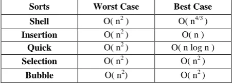
Table 1. Sequential Time complexity of sorting techniques
Sorts Worst Case Best Case
Shell O( n2 ) O( n4/3 )
Insertion O( n2 ) O( n )
Quick O( n2 ) O( n log n )
Selection O( n2 ) O( n2 )
Bubble O( n2) O( n2 )
4.
SOFTWARE REQUIREMENTS
•
Windows 7 Or Windows XP• Secured Shell Client Server(SSH CLIENT FOR WINDOWS):It is a cryptographic network protocol for secured[10] data connection, program executions and remote shell services. It uses public cryptography to authenticate the user.
5.
HARDWARE REQUIREMENTS
Table 2. Hardware Requirements
OS Name Microsoft Windows XP Professional Version 5.1.2600 Service pack 2 Build 2600 System
Manufacturer
LENOVO
System Type X86-based PC
Processor X86 Family 6 Model 23 Stepping 6 Genuine Intel ~2660
Processor X86 Family 6 Model 23 Stepping 6 Genuine Intel ~2660
BIOS Version/Date
LENOVO 51KT54AUS, 1/14/2009
SMBIOS Version
2.5
Locale United States Hardware
Abstraction Layer
Version =
‘5.1.2600.2180{xpsp_sp2_rtm040803-2158}’
Total Physical Memory
2,048.00 MB
Available Physical Memory
1.18 GB
Total Virtual Memory
2.00 GB
Available Virtual Memory
1.96 GB
Page File Space 3.33 GB
6.
BASIC FUNCTIONS OF MPI USED IN
PARALLELIZATION
1. MPI _Init: Initializes the MPI execution environment. This function must be called in every MPI program. It must be called before any other MPI functions and must be called only once in an MPI program. [9]
MPI_Init(&argc,&argv) MPI_INIT (ierr)
2. MPI_Comm_rank: Returns the rank of the calling MPI process within the specified communicator. Initially, each process will be assigned a unique integer rank between 0 and number of tasks - 1 within the communicator MPI_COMM_WORLD. This rank is also referred to as a task ID. If a process becomes associated with other communicators, it will have a unique rank within each of these as well. [9]
MPI_COMM_RANK (comm,rank,ierr)
3. MPI_Comm_size: The MPI_Comm_size function call returns the number of threads or processes being used for this program.[9]
int MPI_Comm_size (MPI_Comm comm,int *size) comm-communicator
size-number of processes in the group of comm(integer) 4. MPI_Finalize: Terminates the MPI execution environment. This function should be the last MPI routine called in every MPI program - no other MPI routines may be called after it.[9]
MPI_Finalize() MPI_FINALIZE (ierr)
5. MPI_Send or MPI_Bcast: Performs a blocking send.[8] int MPI_Send(void *buf , int count, MPI_Datatype datatype, int dest ,int tag, MPI_Comm comm)
buf- initial address of the send buffer(choice) count-number of elements of send buffer datatype- datatype of each send buffer element dest- rank of destination
tag- message tag comm-communicator
6. MPI_Recv or MPI_Reduce: Blocking receive for a message[9]
int MPI_Recv(void *buf , int count, MPI_Datatype datatype, int source ,int tag, MPI_Comm comm,MPI_Status *status) buf- initial address of the receive buffer(choice)
count-maximum number of elements in receive buffer(integer)
datatype- datatype of each receive buffer element status-status object
7. MPI_Scatter: Sends data from one processor to all other processors in a communicator.[9]
int MPI_Scatter(void *sendbuf , int sendcnt , MPI_Datatype sendtype , void *recvbuf , int recvcnt , MPI_Datatype recvtype , int root , MPI_Comm comm)
sendbuf -address of send buffer (choice, significant only at root)
sendcount -number of elements sent to each process (integer, significant only at root)
sendtype -data type of send buffer elements (significant only at root) (handle)
recvcount -number of elements in receive buffer (integer) recvtype -data type of receive buffer elements (handle) root -rank of sending process (integer)
comm -communicator (handle) recvbuf-address of receive buffer
8. MPI_Gather: Gathers together values from a group of processors in the main processor.[9]
int MPI_Gather(void *sendbuf, int sendcnt, MPI_Datatype sendtype, void *recvbuf, int recvcnt, MPI_Datatype recvtype, int root, MPI_Comm comm)
sendbuf -starting address of send buffer (choice) sendcount -number of elements in send buffer (integer) sendtype -data type of send buffer elements (handle)
recvcount -number of elements for any single receive (integer, significant only at root)
recvtype -data type of recv buffer elements (significant only at root) (handle)
root -rank of receiving process (integer) comm -communicator (handle)
recvbuf -address of receive buffer (choice, significant only at root)
9. MPI_Status: It returns the status of the object or task.[9] MPI_Status status
10. MPI_Wtime: It returns the number of clockticks between StartWtime and EndWtime.[9]
MPI_Wtime()
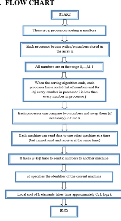
[image:3.595.323.527.376.749.2]7.
FLOW CHART
8.
RUNNING TIME FOR PARALLEL
SORTING
[image:4.595.315.540.83.356.2]p=number of processors n=size of the array t=time in nanoseconds
Table 3. Shell sort parallel running time
n\time p=2 p=3 p=5 p=10 p=20
5000 13 6.45 2.70 1.17 1.52
10000 54 24.8 9.43 3.09 3.25
50000 13 594 216 56.8 30.9
[image:4.595.50.280.165.447.2]100000 53 236 855 221 166
[image:4.595.316.539.399.664.2]Figure 2. Shell sort parallel running time for different number of processors
Table 4. Insertion sort parallel running time
n\time p=2 p=3 p=5 p=10 p=20
[image:4.595.55.280.490.740.2]5000 12.34 5.8062 4.4829 2.7620 1.6839 10000 48.82 22.169 8.4471 4.5878 3.6878 50000 1196 538.14 196.11 51.371 28.171 100000 4822. 2132.4 776.06 198.66 104.59
Figure 3. Insertion sort parallel running time for different number of processors
Table 5. Quick sort parallel running time
n\time p=3 p=5 p=10 p=20 p=30 p=50
5000 0.66 0.71 0.67 1.6 2.87 5.57 10000 1.22 1.06 1.37 1.7 3.53 7.22 50000 6.57 5.04 6.39 5 4.87 6.82 100000 13.0 10.1 8.40 12 9.91 11.2
Figure 4. Quick sort parallel running time for different number of processors
Table 6. Selection sort parallel running time
n\time p=2 p=3 p=5 p=10 p=20
5000 19.888 9.1359 6.1430 4.0287 1.8019 10000 78.531 35.408 13.533 6.3900 3.0760 50000 1963.1 865.06 315.60 81.191 50.507 100000 7849.5 3469.9 1254.0 317.99 241.91
Figure 5. Selection sort parallel running time for different number of processors
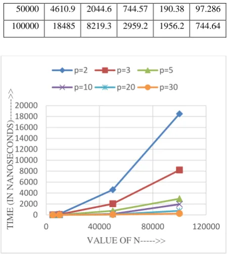
Table 7. Bubble sort parallel running time
n\time p=2 p=3 p=5 p=10 p=20
5000 46.365 20.921 7.7409 6.4089 3.4511 10000 184.59 82.797 30.215 8.2409 7.6010
0 2000 4000 6000 8000 10000 12000 14000 16000 18000
0 50000 100000 150000
T
IM
E
(IN NA
NO
S
ECOND
S
)-->>
VALUE OF N--->>
p=2 p=3 p=5 p=10
0 1000 2000 3000 4000 5000 6000
0 50000 100000 150000
T
IM
E
(IN NA
NO
S
ECOND
S
)
VALUE OF N--->>
p2 p3 p5 p10 p20
0 5 10 15 20
0 50000 100000 150000
T
IM
E
IN NA
NO
S
ECOND
S
---->>
VALUE OF N--->>
p=2 p=3
p=5 p=20
0 2000 4000 6000 8000 10000
0 50000 100000 150000
T
IM
E
IN NA
NO
S
ECOND
S
-->>
VALUE OF N--->>
[image:4.595.54.280.492.738.2] [image:4.595.319.539.712.768.2]50000 4610.9 2044.6 744.57 190.38 97.286 100000 18485 8219.3 2959.2 1956.2 744.64
[image:5.595.315.540.136.453.2]Figure 6. Bubble sort parallel running time for different number of processors
Table 8. Parallel sort with three processors
n\time shell insert quick selection bubble
5000 6.45 5.80 0.66 9.13 20.9219 10000 24.89 22.16 1.22 35.40 82.7970 50000 594.43 538.14 6.57 865.06 2044.64 100000 2369.29 2132.43 13.09 3469.94 8219.30
Figure 7. Parallel sort with three processors
9.
RUNNING TIME FOR SEQUENTIAL
SORTING
Table 9. Sequential Sort (time in nanoseconds)
n\(time X
106) shell insert quick selection bubble
1000 1 1 1 2 3
5000 22 23 1 38 68
10000 105 73 2 153 274
50000 2186 1765 9 3831 7727
100000 9080 7149 17 15309 31400
Figure 8. Sequential Sort (time in nanoseconds)
10.
CONCLUSION
Hence it is inferred that parallel sorting is much faster than sequential sorting. Although bubble sort algorithm is the slowest one compared with selection sort, shell sort, insertion sort and quick sort, its execution time decreased rapidly as the number of processes increased even the number of processes is greater than the number of physical cores. This is because it does not require heavy communication; the great part of the execution time is consumed in computations. So as the number of processes increases the amount of work done by each process will be decrease regardless the effect of the number of physical cores used. So as number of processors increase, time taken to solve the computations still dominates over the communication time as by increasing number of processors tasks are more divided so overall time decreases. Selection Sort also has the same behavior in contrast to this situation the execution time of quick sort was very sensitive to the number of running processes. The total overhead generated from processes initialization and inter-process communication negatively affects the execution time. Although quick sort is the fastest one among the five algorithms, it suffers from a high communication overhead cost and load imbalance compared with other sorting techniques.
The advantage of Shell sort over Insertion Sort is that items are moved closer to their final position with fewer exchanges
0 2000 4000 6000 8000 10000 12000 14000 16000 18000 20000
0 40000 80000 120000
T
IM
E
(IN NA
NO
S
ECOND
S
)--->>
VALUE OF N--->>
p=2 p=3 p=5
p=10 p=20 p=30
0 2000 4000 6000 8000 10000
0 50000 100000 150000
T
IM
E
(IN NA
NO
S
ECOND
S
)--->>
VALUE OF N--->>
SHELL SORT INSERTION SORT
QUICK SORT SELECTION SORT
BUBBLE SORT
0 10 20 30 40
0 50000 100000 150000
T
IM
E(I
N
S
ECOND
S
)--->>
VALUE OF N--->>
SHELL SORT INSERTION SORT
QUICK SORT SELECTION SORT
[image:5.595.53.275.364.692.2]of items. While Insertion Sort exchanges adjacent items, Shell sort exchanges "adjacent" items that are actually h items apart. The parallel and sequential timing on separate graphs were compared which showed that sequential time is 105 times greater than parallel time.
11.
REFERENCES
[1] Narayan Desai, Andrew Lusk, Rick Bradshaw, Ewing Lusk, “MPISH: A Parallel Shell for MPI Programs”, 19th IEEE International Parallel and Distributed Processing Symposium (IPDPS’05), pp. 1530-2075 [2] Fangfa Fu, Siyue Sun, Xin'an Hu, Junjie Song, Jinxiang
Wang and Minyan Yu, “MMPI: A Flexible and Efficient Multiprocessor Message Passing Interface for NoC-Based MPSoC”, IEEE, 2010, pp. 359-362
[3] Jesper Larsson Träff, William D. Gropp and Rajeev Thakur, “Self-Consistent MPI Performance Guidelines”, IEEE TRANSACTIONS ON PARALLEL AND DISTRIBUTED SYSTEMS, May 2010,vol 21, pp. 698-709
[4] Zhongxiao Zhao, Chen Min and Fuzhou, “An Innovative Bucket Sorting Algorithm Based on Probability Distribution”, World Congress on Computer Science and Information Engineering, 2009, pp. 846-850
[5] Adeel Abbas, Affan Ahmad, “Object Oriented Parallel Programming”, IEEE, 2002, pp. 89-93
[6] Xiao-ping LIU, En-zhu WANG, Li-ping ZHENG, Xing-wu WEI,” Study on Template for Parallel Computing in Visual Parallel Programming Platform”, 1 st International Symposium on Pervasive Computing and Applications, 2006, pp. 476-481
[7] Sequential and parallel sorting algorithms
http://www.iti.fh-flensburg.de/lang/algorithmen/sortieren/algoen.htm [8] LINUX MAGAZINE-MPI in Thirty Minutes
http://www.linux-mag.com/id/5759/
[9] Message Passing Interface (MPI) Author: Blaise Barney, Lawrence Livermore National Laboratory
[10]R. S. RamPriya, M. A. Maffina, “A Secured and Authenticated Message Passing Interface for Distributed Clusters”, SPSymposium, IIITD, 2013
[11]Wang Xiang, “Analysis of the Time Complexity of Quick Sort Algorithm”, IEEE, 2011, pp. 408-410 [12]Keliang Zhang,”A Novel Parallel Approach of Radix