Research Article
CODEN(USA) : JCPRC5
ISSN : 0975-7384
Sliding mode control of bus stability based on LMI
Liao Cong
1, Wu Xinye
2*and Huang Hongwu
11
Dep. of Mechanical and Electrical Engineering, Xiamen University, Xiamen, China
2Dep. of Civil Engineering, Xiamen University, Xiamen, China
_____________________________________________________________________________________________
ABSTRACT
In order to improve steering stability of the vehicle, a 3-DOF bus rollover dynamics model is established,and the
vehicle steering stability controller is designed, and a kind of easy sliding mode control strategy based on linear matrix inequality (LMI) is proposed. Using Matlab/Simulink, the simulation results show that the proposed sliding mode control strategy can effectively reduce roll angle velocity, roll angle, side-slip angle and stable yaw rare, and thus improve the vehicle steering stability.
Key words: Information fusion; granular computing; intelligent transportation
_____________________________________________________________________________________________
INTRODUCTION
The rollover stability has become the focus of the world automobile research in recent years.Differential braking can reduce the inhibition of lateral acceleration, yaw velocity and does not change the purpose of the driver, but the cost is low.Therefore,using differential braking to improve the vehicle roll stability is a better choice.The paper [1] has proposed a nonlinear asymptotic tracking control strategy to ensure the reference yaw angle control strategy to prevent rollover. The paper [2] has improved the stability of the car through direct yaw moment control, using optimal LQR control strategy. The paper [3] has established a nonlinear vehicle model developing a differential braking stability control and a fuzzy logic controller. The paper [4]has built a vehicle stability control by using model predictive control theory framework tolimit the maximum roll angle of the car. The linear matrix inequality (LMI) used in this paper is a powerful tool for the design of control field, to construct the effective computer algorithm for solving problems[5]. Before the linear matrix inequality (LMI) are widely used in control ,most problems are solved by method of Riccati equation or inequality method [6-8].In the processing of the solution of the Riccati equation or inequality, there are a large number of parameters and the positive definite symmetric matrices to be adjusted. The linear matrix inequality method can make up the shortcomings of Riccati equation method.
The sliding mode variable structure control algorithm has little dependence, good robustness and strong anti-interference ability in all control algorithms, and the variable structure control based on the LMI (linear matrix inequality) has some advantages on both the LMI and sliding mode variable structure control. In this paper the LMI design of sliding mode control will be applied to improve vehicle stability by using differential brake and sliding mode control strategy, and thus effectively improvesthe anti-rollover performance of bus and enhances the bus stability.
Vehicle dynamics model
Fig. 1 Vehicle dynamics model
(1) ignores the effect of air force. (2) does not consider the road input.
(3) does not consider the influence of pitch motion.
(4) ignore the non sprung mass because non sprung mass relative is relatively small to the sprung mass. (5) the vehicle suspension is equivalent to the anti roll spring and damping.
(6) roll angle, yaw angle and tire angle are calculated to micro small steering. (7) the tire characteristics in the linear relationship.
As shown in Figure 1, The automobile's steering wheel movement dynamics equations are: (1)Lateral movement
(
)
(
)
y r f
y f r f
V
k b k a
mV
k
k
mV
m h
k
V
γ
φ
V
γ
δ
• • ••
−
•+
+
+
=
+
+
(1)(2)Roll motion
(
)
(
)
y r f
x f r f
V
k b k a h
I
C
K
mg h
k
k h
k h
V
V
φ φ
φ
••+
φ
•+
φ
=
φ
−
+
+
−
γ
•+
δ
(2)(3)Yaw motion
2 2
f r r f
z y f
k a
k b
k b
k a
I
V
k a
V
V
γ
••+
+
γ
•=
−
+
δ
(3)Where:
m——Vehicle mass,
V
、
Vy——Vehicle instantaneous velocity, lateral velocity,γ
•——Vehicle Yaw rate,h —— the distance from the center of gravity to the roll center,
φ
—— the roll Angle displacement,δ—— The front wheel steering angle,
Ix、Iy、Iz—— The vehicle moment of inertia around the X, y, Z axis,
K
φ—— Suspension roll stiffness in the roll direction,C
φ—— damping of roll direction,a、b—— The distance from vehicle gravity to the front and rear axle, γ
B —— Vehicle track,
kf、kr—— The front, rear tire stiffness.
According to the equation (1), (2), (3), taking system state variables to:
[
]
TX
β γ φ φ
• •=
, andconsidering the additional yaw moment of the differential braking, then the system state equation can be written as:
1 1
( )
( )
( )
( )
X t
•=
AX t
+
BU t
+
BU t
(4)Where:
)
(
1t
U
——the known input matrix,[ ]
1
( )
( )
U t
=
δ
t
,( )
U t
——the control input matrix,[ ]
1
( )
( )
U t
=
u t
, is the control force of yaw moment.2 2 2
2 2
(
)(
)
(
)(
)
(
)
0
0
(
)
(
)
0
0
1
0
x f r x r f
x x x x
r f f r
z z
f r r f
x x x x
I
mh
k
k
I
mh
k b k a
hC
mgh
K h
V
mVI
mVI
I
I
k b k a
k a
k b
A
I
I V
h k
k
h k b k a
C
mgh
K
I V
I V
I
I
φ φ φ φ
+
+
+
−
−
−
−
−
−
−
+
=
+
−
−
−
−
, 2 1(
)
0
Tx f f f
x z x
I
mh k
k a
k h
B
I mV
I
I
+
=
,0
0
0
2
T zB
B
I
=
−
.Sliding mode control strategy of braking differential
Define a Factor in determining rollover - lateral load transfer ratio[9] for vehicle rollover stability of the state of the evaluation index, lateral load transfer ratio expressions for:
zR zL
zR zL
F
F
F +F
LTR
=
−
(5)Where:
FzR---the right wheel contact with the ground force; FzL--- the left wheel contact with the ground forces.
About under the stable state of straight, if the left mass and right mass is symmetrical, FzL = FzR, then LTR = 0; If left or right side of the wheel is raised off the ground, the FzL = 0 or FzR = 0, so LTR = 1 or - 1; Without the wheels from the ground up the |LTR | < 1, the automobile in side tumbling stability state; And | LTR | value is smaller, the better side tumbling stability of vehicle. According to the theory of a rollover, dynamic lateral load transfer ratio can be expressed as [10] :
2(
C
K
)
LTR
mgB
φ
φ
φφ
•
+
=
(6)Where:Differential braking control has changed the current dynamic characteristics of automobile, but also changed the steering characteristic of vehicle. Changes on vehicle dynamic characteristics are to reduce vehicle speed, changes on the steering characteristics of vehicle has produced over-steering or under-steering of the automobile, according to "friction ellipse theory", increased the longitudinal force, reduced lateral force, and reducing the lateral acceleration, thus lowering the risk of low rollover.
The sliding mode controller is shown in Figure 2, get the sliding mode control law through the state
equation. The definition of the sliding mode function is
s
=
B Px
T , P is4 4
×
positive definite matrix, get s=0 through the design of P[7]. To get P by using the linear matrix inequality, the equation of state (4) written as follows:( )
( )
[ ( )
( , )]
x t
Ax t
B u t
f x t
•=
+
+
(7)f(x,t) is the uncertain disturbance, and meet a certain intensity limit, |f(x,t)|≤δf,
Design of sliding mode controller:
( )
eq swu t
=
u
+
u
(8)Equivalent control
u
eq= −
(
B PB
T)
−1B PAx t
T( )
, (9)Switching control
u
sw= −
(
B PB
T)
−1[ B PB
Tδ ε
f+
0]sgn s
( )
,ε0>0.A control law is [16]:
( )
(
eq sw)
( )
u t
= −
Kx
+
Kx
+
u
+
u
= −
Kx
+
v t
, (10)(7) into:
( )
( )
(
( , ))
x t
Ax t
B v
f x t
•=
+
+
,A
= −
A BK
, The design of K allows for Hurwitz stable matrix, so asto ensure the stability of the closed-loop system.
The Lyapunov function: T
V
=
x Px
, (11)2
T2
T( )
2
T(
( , ))
V
x P x
x P Ax t
x PB v
f x t
• •
=
=
+
+
, (12)The previous
s
=
B Px
T=
0
, sos
T=
x PB
T=
0
,The above formula is:2
T T(
T)
V
x P Ax
x
P A
A P x
•=
=
+
, (13)In order to set up
V
0
•<
, so:0
T
P A
+
A P
<
, so:(
) (
)
T0
P A BK
−
+
A BK
−
P
<
, (14)X is written as
X
=
P
−1, On the left and right multiplication by type X transposition to above formula:(
)
T T T
AX
+
XA
<
BKX
+
KX
B
, KX is written as KX=Y, so:T T T
AX
+
XA
<
BY
+
Y B
, (15)In order to ensure that P is a symmetric positive definite matrix, so:
0
T
simplified. And obtained K by pole command place in MATLAB, and then obtained P through the LMI toolbox , completed the design of sliding mode controller.
Fig. 2 Principle diagram of sliding mode control
The simulation and results analysis
The simulation is under the Matlab/simulink, vehicle parameters are as follows: m=1320kg; g=9.81m/s2; h=0.36m; Ix=358.2kg.m
2
; Iz=1268 kg.m 2
; Cφ=3950N.m.s/rad; Kφ=35086N.m.s/rad; a=1.08m; b=1.26m; B=1.5m; kf=90320N.m.s/rad; kr=180600N.m.s/rad.
The car speed is 144km / h, the steering wheel stability angle is 40 degrees, the input signal is a step simulation signal, the role of the time is the end of 1s, simulated vehicle running at a speed in the corners of steady state, using sliding mode control law formula (6), on the LMI-based sliding Mode Control and uncontrolled contrast to simulation, taking δf = 0.1, ε0 = 0.2, instead of the sign function with saturation function, taking the thickness of the boundary layer
∆ =
0.05
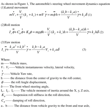
, after repeated testing, pole configuration is selected [-16 +2 * i, -16-2 * i, -600 +2 * i, -600-2 * i], the simulation results are shown in Figure 3 to 7.Fig. 3 Curves of roll anglevs time
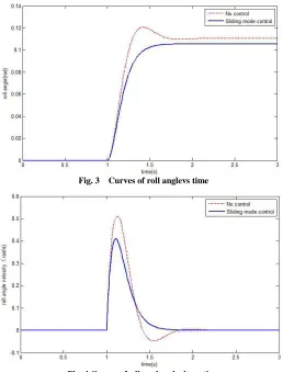
[image:5.595.210.381.114.199.2] [image:5.595.175.433.367.706.2]Fig. 5 Curves of Lateral load transfer ratiovs time
Fig. 6 Yaw velocityvs time
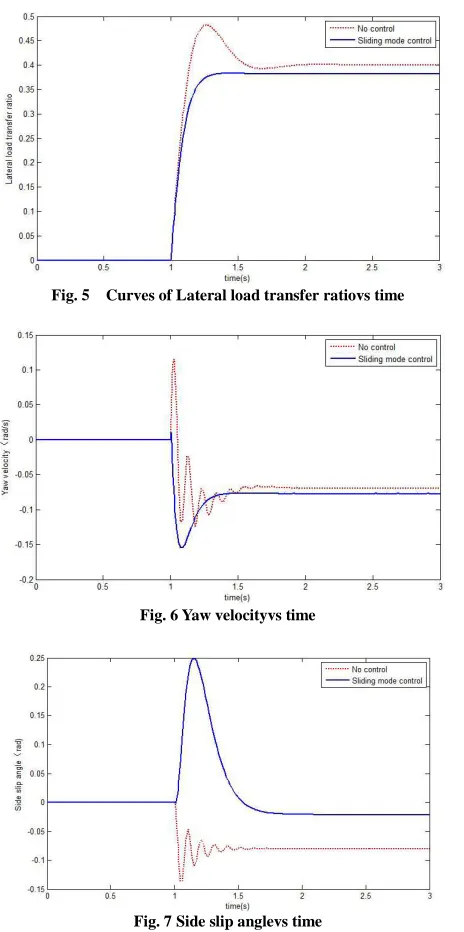
Fig. 7 Side slip anglevs time
The root mean square values are shown in table 1.Through contrast of the sliding mode control based on LMI and no control, can be seen from the table 1, roll angle root mean square value of sliding mode control is reduced by 7.43% than no control, roll angular velocity root mean square value of sliding mode control is reduced by 20.30% than no control, lateral load transfer ratio root mean square value of sliding mode control is reduced by 7.44% than no control, yaw rate root mean square value of sliding mode control is increased by 12.19% than no control, Sideslip angle root mean square value of sliding mode control is reduced by 10.13% than no control.
From Fig. 6,yaw velocity root mean square value has increased, but in the allowed range, other each response performance indexes have great improvement, that shows good control performance of the sliding mode controller .
Tab.1 Root mean square comparison of results
root mean square value no control sliding mode control
roll angle(rad) 0.0982 0.0909
roll angular velocity (rad/s) 0.1384 0.1103 lateral load transfer ratio 0.3694 0.3419
yaw rate (rad/s) 0.0689 0.0773
[image:6.595.194.418.675.749.2]CONCLUSION
Through analysis and study of anti-rollover control system of sliding mode control for vehicle differential braking, establish the vehicle model, and propose the sliding mode control design and simulation research of sliding mode control strategy, draw the following conclusions:
(1) A sliding mode controller of good control performance is designed based on LMI, improve vehicle stability, and improve vehicle rollover state. The reasonable application of differential braking control method can improve the vehicle braking stability.
(2)The simulation results show that: to design a controller using the LM method, and the use of MATLAB in the LMI toolbox, the method is simple, easy to implement, the sliding mode control can achieve good performance. (3)Compared to semi-active / active suspension with lower reaction times , The stability of differential braking control has the advantages fast and easy to realize.But compared to anti rollover on semi-active / active suspension, differential braking control of anti rollover torque limited within a certain range, the control effect is not as good as semi-active / active suspension.
(4)The differential braking control has many ways to apply, the wheel braking force distribution should be paid attention to when differential braking is applied. (Electromechanic Brake (EMB) has rapid response speed, conducive to energy conservation and environmental protection, is a kind of method to realize easily.
Acknowledgments
It is a project supported by the National Natural Science Foundation (51305372).
REFERENCES
[1]Schofield B, Hagglund T, Rantzer A. Vehicle dynamics control and controller allocation for rollover prevention[C]Computer Aided Control System Design, 2006 IEEE International Conference on Control Applications,
2006 IEEE International Symposium on Intelligent Control, 2006 IEEE. IEEE, pp. 149-154,2006.
[2]A.GOODARZI,M.ALIREZAIE.International Journal of Automotive Technology, Vol. 10, No. 5, pp.567−575,2009.
[3]Zhao C, Xiang W, Richardson P. Vehicle lateral control and yaw stability control through differential braking[C]Industrial Electronics, 2006 IEEE International Symposium on. IEEE, pp. 384-389,January, 2006. [4]Carlson C R, Gerdes J C. Optimal rollover prevention with steer by wire and differential braking[C]Proceedings
of IMECE. pp. 16-21,2003.
[5] Liu Jinkun. MATLAB simulation for sliding mode control [M]. Beijing: Tsinghua University press, 2012. [6]Petersen I R, Hollot C V. A Riccati equation approach to the stabilization of uncertain linear systems[J].
Automatica, v.22,n.1,pp. 397-411,1986.
[7]Mahmoud M S, Al-Muthairi N F. Quadratic stabilization of continuous time systems with state-delay and norm-bounded time-varying uncertainties[J]. Automatic Control, IEEE Transactions on,
v.39,n10,pp.2135-2139,1994.
[8]Xie L, Soh Y C, de Souza C E. Robust Kalman filtering for uncertain discrete-time systems[J]. Automatic
Control, IEEE Transactions on,v. 39,n.6,pp.1310-1314,1994,.
[9]Solmaz S, Corless M, Shorten R. A methodology for the design of robust rollover prevention controllers for automotive vehicles: Part 1-Differential Braking[C]Decision and Control, 2006 45th IEEE Conference on. IEEE, pp. 1739-1744,2006.
VasiliosTsourapas, DamrongritPiyabongkarn, Alexander C. Williams, et al.New Method of Identifying Real-Time
Predictive Lateral Load Transfer Ratio for Rollover Prevention Systems[C]. 2009 American Control Conference