Dynamic Programming to Identification Problems

ISSN Online: 2331-4249 ISSN Print: 2331-4222

Dynamic Programming to

Identification Problems

Nina N. Subbotina

, Evgeniy A. Krupennikov

1_{Krasovskii Institute of Mathematics and Mechanics, Ekaterinburg, Russia} 2_{Ural Federal University, Ekaterinburg, Russia}

Abstract

An identification problem is considered as inaccurate measurements of dynamics on a time interval are given. The model has the form of ordinary differential equations which are linear with respect to unknown parameters. A new approach is presented to solve the identification problem in the framework of the optimal control theory. A numerical algorithm based on the dynamic programming method is suggested to identify the unknown parameters. Results of simulations are exposed.

Keywords

Nonlinear System, Optimal Control, Identification, Discrepancy, Dynamic Programming

1. Introduction

Mathematical models described by ordinary differential equations are considered. The equations are linear with respect to unknown constant parameters. Inaccurate mea-surements of the basic trajectory of the model are given with known restrictions on admissible small errors.

The history of study of identification problems is rich and wide. See, for example, [1] [2]. Nevertheless, the problems stay to be actual.

In the paper a new approach is suggested to solve them. The identification problems are reduced to auxiliary optimal control problems where unknown parameters take the place of controls. The integral discrepancy cost functionals with a small regularization parameter are implemented. It is obtained that applications of dynamic programming to the optimal control problems provide approximations of the solution of the identifi-cation problem.

See [3] [4] to compare different close approaches to the considered problems.

How to cite this paper: Subbotina, N.N. and Krupennikov, E.A. (2016) Dynamic Program- ming to Identification Problems. World Jour- nal of Engineering and Technology, 4, 228-234.

http://dx.doi.org/10.4236/wjet.2016.43D028

2. Statement

We consider a mathematical model of the form

* 0

( )

( ) ( , ( )) , [ , ],

dx t

F t G t x t k t t T

dt = + ∈ (1)

where n

x∈R is the state vector, *

m

k ∈R , m≥n is the vector of unknown para-

meters satisfying the restrictions

*

| i| , = 1, , .

K≤ k ≤K i  m (2)

Let the symbol ||k|| denote the Euclidean norm of the vector k= ( ,k1 ,km).

It is assumed that a measurement ( ) : [ , ]0

n

yδ ⋅ t T →R of a realized (basic) solution

*( ), [0, ]

x t t∈ T of Equation (1) is known, and

*

|| ( )y t −x t( ) ||≤δ, ∀ ∈t [0, ].T (3)

We consider the problem assuming that the elements g t x i_ij( , ), = 1,, ,n j= 1,, ,m

of the n m× matrix G t x( , ) are twice continuously differentiable functions in Rn+1.

The coordinates y_iδ( ), = 1,⋅ i , ,n of the measurement yδ( )⋅ are twice continuously

differentiable functions in [0, ]T , too. The coordinates f t ii( ), = 1,,n of the vector-

function F t( ) are continuous functions on the interval [0, ]T .

We assume also that the following conditions are satisfied

.1

A There exists such constants Y > 0 and δ0> 0 that for all δ δ≤ 0 the

inequalities

2

0 2

( ) ( )

| ( ) | , i , i , = 1, , , [ , ]

i

dy t d y t

y t Y Y Y i n t t T dt dt

δ δ

δ _{≤ ≤ ≤ ∀  ∈ (4)}

are true.

.2

A There exist such constant r>2δ₀ (δ0 from A.1) and such compact set [0, ]T Rn

Ω ∈ × that for any 0 <δ δ≤ 0 the following conditions are held

{( , ) : ||t y y−y tδ( ) ||≤r, t∈[0, ]}T ∈ Ω;

( , ) > 0, || ||> 0, ( , )

s Q t x sΤ as s t x ∈ Ω.

Here Q t x( , ) =G t x G t x( , ) ( , ) = (q t xij( , )), = 1,i , ,n j= 1, ,m

Τ _{  .}

The identification problem is to create parameters kδ such, that

* *

[0, ]

|| ( ) ( ) || =C max|| ( ) ( ) || 0, 0, t T

xδ x x tδ x t asδ

∈

⋅ − ⋅ − → → ₍₅₎

where xδ( )⋅ is the solution of Equation (1), as k=kδ.

3. Solution

3.1. An Auxiliary Optimal Control Problem

Let us introduce the following auxiliarly optimal control problem for the system

0 ( )

= ( ) ( , ( )) , [ , ],

dx t

F t G t x t u t t T

dt + ∈ (6)

where m

= { m:| _i| , = 1, , }

u∈U u∈R u ≤K i  m (7)

for a large constant K> 0.

Admissible controls are all measurable functions u( )⋅ . For any initial state

0 0

( ,_{t x} )_∈[0, ]_{T ×R}n, the goal of the optimal control problem is to reach the state

( , ( ))T y T

and minimize the integtal discrepancy cost functional

0 0 0 2 2 2 , || ( ) ( ) || ( ( )) = [ || ( ) || ] . 2 2 T t x t

x t y t

I u ⋅

∫

Here y t( ) =y tδ( ) is the given measurment; α2 is a small regularization parameter,

0 0 ( )) = ( ; , , ( ))

x t x t t x u ⋅ is the trajectoty of the system (6), (7) generated under an

admissible control u( )⋅ out the initial point x0. The sign minus in the integrand

allows to get solutions which are stable to perturbations of the input data.

N o t e 1. A solution _uδ α, _{( )⋅} of the optimal control problem (6), (7), (8) allows us to construct the averaging value k( , )δ α

0 , 0 1 ( , ) = ( ) T t

k u t dt

T t

δ α δ α

−

∫

which can be considered as an approximstion of the solution of the identification problem (1), (2).

3.2. Necessary Optimality Conditions: The Hamiltonian

Recall necessary optimality conditions to problem (6), (7), (8) in terms of the hami- ltonian system [5] [6].

It is known that the Hamiltonian Hα( , , )t x s to problem (6), (7), (8) has the form

2 2

2 || ( ) ||

( , , ) =min[ ( , ) || || ] ( ),

2 2

u U

x y t

Hα t x s s G t x uΤ α u s F tΤ

∈

−

+ − +

where n

s∈R is an ajoint variable, the symbol Τ denotes the transpose operation.

It is not difficult to get

2 2

, , 2 || ( ) ||

( , , ) = [ ( , ) || || ] ( ).

2 2

x y t

Hα t x s s G t x uΤ α δ +α uα δ − − +s F tΤ

where , ,

= ( _i ( , , ), = 1, , ) :

uα δ uα δ t x s i  m

,

, ( , , ) ,

( , , ) = ( , , ), ( , , ) [ , ],

, ( , , ) .

i

i i i

i

K if r t x s K

u t x s r t x s if r t x s K K

K if r t x s K

α

α δ α α

α  − ≤ −  _{∈ −}   _≥ 

Here the vector-column rα( , , ) = (t x s r_iα( , , ), = 1,t x s i , )m has the form

2 1

( , , ) = ( , ) .

rα t x s G t x s

α Τ

− ₍₁₀₎

3.3. The Hamiltonian System

Necessary optimality conditions can be expressed in the hamiltonian form. An optimal trajectory 0

( )

(7), (8) have to satisfy the hamiltonian system of differential inclusions

0 ( , , ), ( , , ), = 1, , , [ , ],

i i

s_i x_i

dx ds

H t x s H t x s i n t t T

dt dt

α α

∈ ∂ ∈ −∂  ∈ (11)

and the boundary conditions

( , ) = ( ), ( , ) = , = 1, , .

i i i i

x T ξ y T s T ξ ξ i  n (12)

where symbols ( , , ), ( , , )

i i

s x

Hα t x s Hα t x s

∂ ∂ _{denote Clarke’s subdifferentials [7] and} 0_{( ) = ( , )}

x t x t ξ , _{u t}0_{( ) =u}α δ, _{( , ( , ), ( , ))t x t}ξ _{s t} ξ .

Parameters ξi belong to the intervals Si δ = [si min,si max] where values si min and i max

s are choosen from the conditions

( ) ( )

|dx Ti dy Ti | , _i 1,..., ._n

dt − dt ≤δ = (13)

We introduce the last important assumption.

.3

A There exists a constant 0< =S S(δ₀) such that restrictions on controls in

problem (6), (7), (8) satisfy the relations

( , , ) [ , ], 1, , ,

i

rα t x s ∈ −K K i=  m (14)

2 2

( , )t x , |sj| 2

α

α

∀ ∈ Ω ∀ ≤ ∈ = 

where r_iα( , , ),t x s i=1,,m are from (10).

N o t e 2. Using definition (10) one can check that constant K, satisfying assumtion

.3

A , K can be taken as

0 2 ( )

K= GQ Y+ +F δ ,

where



max{ ( ) : [0, ], 1,..., },

max{| ( , ) |: ( , ) , 1,..., , 1,..., } ,

max{| ( , ) |: ( , ) , 1,..., , 1,..., }. i

ij

ij

F F t t T i n

G g t x t x i n j m Q q t x t x i n j m

= ∈ =

= ∈ Ω = =

= ∈ Ω = =

Hereg t x iij( , ), =1,..., ,n j=1,...,m are components of matrix G t x( , ) and  _{( , ), 1,..., , 1,...,}

ij

q t x i= n j= m are components of matrix 1 ( , )

Q− t x .

If ( , )t x ∈ Ω and |sj| 2≤

α

α

simple form

2

2

1 || ( ) ||

( , , ) = [ ( , ) ( , ) ] ( )

2 2

x y t

Hα t x s s G t x G t x s s F t

α

Τ Τ − Τ

− − +

and the differential inclusions (11) transform into the ODEs.

0 ( , , ) ( , , )

= , = , = 1, , , [ , ],

i i

i i

dx H t x s ds H t x s

i n t t T

dt s dt x

α α

∂ ₋∂ _∈

∂ ∂  (15)

Let us introduce the discrepancies z t( ) = ( )x t −y t( ), and obtain from (15) the

following equations 2 2 1 ( ) = ( ) ( , ( )) ( ) ( ), ( , ( ) 1

( ) = ( ) ( )( ij ) ( ), = 1, , ,

i i

i

z t F t Q t x t s t y t q t x t

s t z t s t s t i n x α α Τ − − ∂ + ∂  

and the boundary conditions

( ) = 0, ( ) = , = 1, , ,

i i i

z T s T ξ i  n (17)

where ξ saisfy (13).

3.4. Main Result: Dynamic Programming

Using skims of proof for similar results in papers [8] [9] [10] we have provided the following assertion.

Theorem 1 Let assumptions A.1−A.3 be satisfied and the concordance of para-

meters α δ, : 2 0, 0

/ = 0

lim

δ→ α→δ α takes place, then solutions of problem (11), (12), (13)

, ,

( , ), ( , )

xδ α t ξ sδ α t ξ are extendable and unique on [0, ]T for any ξ_i saisfying (13)

and

,

* 0, 0

|| ( , ) ( ) || = 0.

lim x t x t C

δ α

δ→ α→ ξ − (18)

It follows from theorem 1, that the average values k( , )δ α (9) obtained with the

help of dynamic programmig satisfy the desired relation

*

( , ) , 0, 0.

kδ α →k asδ → α → (19)

4. Numerical Example

A series of numerical experiments, realizing suggested method, has been carried out. As an example a simple mechanical model has been taken into consideration.

This simplified model describes a vertical rocket launch after engines depletion. The dynamics are described as

( ) = ( ) , [0, 4],

x t −kx t −g t∈

  (20) where x( )⋅ is a vertical coordinate of the rocket, k is an unknown windage

coefficient and g =9.8 is a free fall acceleration.

A function yδ( )t is known and satisfies assumption A.1. This function was

obtained by random perturbing of the basic solution x t*( ) for k* =0.3.

The suggested method is applied to solve the identification problem for k* = 0.3.

We introduce new variables x t1( ) = ( ),x t x t2( ) =x t1( ) = ( )x t and transform Equation

(20) into

1( ) = 2( ) ( ),1 2( ) = 2( ) ( )1 , [0, 4],

x t x t u t x t −u t x t −g t∈ (21)

where u t2( )=k t( ) and u t1( ) is a fictitious control, which was introduced in order to

get m n× matrix G t x t( , ( )) in (1) satisfying dimentions restriction m≥n.

We put y t2( ) = y t1( ).

The corresponding hamiltonian system (16) for problem (21),(8) has the form

2 2 2 2

1 1 2 2 2 1

2 2 2 2

1 2 1 1 1 2 1 2 2 2

( ) = ( ) ( ) / , ( ) = ( ) ( ) / ,

( ) = ( ) ( ) / ( ( ) ( )), ( ) = ( ) ( ) / ( ( ) ( ))

x t s t x t x t s t x t g

s t s t x t x t y t s t s t x t x t y t

α α

α α

− − −

+ − + −

 

  (22)

with initial conditions

2 2

1( ) = 1( ), 2( ) = 2( ), 1( ) = 0, 2( ) = ( 2( ) ) / 1( ).

x T y T x T y T s T s T −α y T +g y T (23)

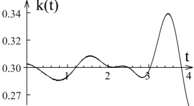
Figure 1. k(t) graph for δ = 5; k(α, δ) = 0.375.

Figure 2. k(t) graph for δ = 2; k(α, δ) = 0.325.

of functions u t2( )=k t( ) are exposed. The graphs illustrate convergence of the

suggested method. The calculated corresponding average values (9) are exposed as well.

Acknowledgements

This work was supported by the Russian Foundation for Basic Research (projects no. 14-01-00168 and 14-01-00486) and by the Ural Branch of the Russian Academy of Sciences (project No. 15-16-1-11).

References

[1] Billings, S.A. (1980) Identification of Nonlinear Systems—A Survey. IEE Proceedings D— Control Theory and Applications, 127, 272-285. http://dx.doi.org/10.1049/ip-d.1980.0047

[2] Nelles, O. (2001) Nonlinear System Identification: From Classical Approaches to Neural Networks and Fuzzy Models. Springer, New York.

http://dx.doi.org/10.1007/978-3-662-04323-3

[3] Kryazhimskiy, A.V. and Osipov, Yu.S. (1983) Modelling of a Control in a Dynamic System.

Engrg. Cybernetics, 21, 38-47.

[4] Osipov, Yu.S. and Kryazhimskiy, A.V. (1995) Inverse Problems for Ordinary Differential Equations: Dynamical Solutions. Gordon and Breach, London.

[5] Pontryagin, L.S., Boltyanskij, V.G., Gamkrelidze, R.V. and Mishchenko, E.F. (1962) The Mathematical Theory of Optimal Processes. Interscience Publishers, a Division of John Wi-ley and Sons, Inc., New York and London.

[6] Krasovskii, N.N. and Subbotin, A.I. (1977) Game Theoretical Control Problem. Springer- Verlag, New York.

York.

[8] Subbotina, N.N., Kolpakova, E.A., Tokmantsev, T.B. and Shagalova, L.G. (2013) The Me-thod of Characteristics to Hamilton-Jacobi-Bellman Equations (Metod Harakteristik Dlja Uravnenija Gamil’tona-Jakobi-Bellmana) (in Russian). Ekaterinburg: RIO UrO RAN. [9] Subbotina, N.N., Tokmantsev, N.B. and Krupennikov, E.A. (2015) On the Solution of

In-verse Problems of Dynamics of Linearly Controlled Systems by the Negative Discrepancy Method. Optimal Control, Collected Papers. In Commemoration of the 105th Anniversary of Academician Lev Semenovich Pontryagin, Tr. Mat. Inst. Steklova, 291 MAIK. Nauka/ Interperiodica, Moscow.

[10] Subbotina, N.N. and Tokmantsev, N.B. (2015) A Study of the Stability of Solutions to In-verse Problems of Dynamics of Control Systems under Perturbations of Initial Data. Pro-ceedings of the Steklov Institute of Mathematics December 2015, 291, 173-189.

http://dx.doi.org/10.1134/s0081543815090126

Submit or recommend next manuscript to SCIRP and we will provide best service for you:

Accepting pre-submission inquiries through Email, Facebook, LinkedIn, Twitter, etc. A wide selection of journals (inclusive of 9 subjects, more than 200 journals)

Providing 24-hour high-quality service User-friendly online submission system Fair and swift peer-review system

Efficient typesetting and proofreading procedure

Display of the result of downloads and visits, as well as the number of cited articles Maximum dissemination of your research work

Submit your manuscript at: http://papersubmission.scirp.org/