http://www.scirp.org/journal/am ISSN Online: 2152-7393 ISSN Print: 2152-7385
An Effective Numerical Calculation
Method for Multi-Time-Scale
Mathematical Models
in Systems Biology
Yohei Motomura1, Hiroyuki Hamada1,2, Masahiro Okamoto1,2
1Graduate School of Systems Life Sciences, Kyushu University, Fukuoka, Japan 2Synthetic Systems Biology Research Center, Kyushu University, Fukuoka, Japan
Abstract
The improvements of high-throughput experimental devices such as microarray and mass spectrometry have allowed an effective acquisition of biological comprehensive data which include genome, transcriptome, proteome, and metabolome (multi- layered omics data). In Systems Biology, we try to elucidate various dynamical cha-racteristics of biological functions with applying the omics data to detailed mathe-matical model based on the central dogma. However, such mathemathe-matical models possess multi-time-scale properties which are often accompanied by time-scale dif-ferences seen among biological layers. The difdif-ferences cause time stiff problem, and have a grave influence on numerical calculation stability. In the present conventional method, the time stiff problem remained because the calculation of all layers was im-plemented by adaptive time step sizes of the smallest time-scale layer to ensure sta-bility and maintain calculation accuracy. In this paper, we designed and developed an effective numerical calculation method to improve the time stiff problem. This method consisted of ahead, backward, and cumulative algorithms. Both ahead and cumulative algorithms enhanced calculation efficiency of numerical calculations via adjustments of step sizes of each layer, and reduced the number of numerical calcu-lations required for multi-time-scale models with the time stiff problem. Backward algorithm ensured calculation accuracy in the multi-time-scale models. In case stu-dies which were focused on three layers system with 60 times difference in time-scale order in between layers, a proposed method had almost the same calculation accura-cy compared with the conventional method in spite of a reduction of the total amount of the number of numerical calculations. Accordingly, the proposed method is useful in a numerical analysis of multi-time-scale models with time stiff problem. How to cite this paper: Motomura, Y.,
Hamada, H. and Okamoto, M. (2016) An Effective Numerical Calculation Method for Multi-Time-Scale Mathematical Models in Systems Biology. Applied Mathematics, 7, 2241-2268.
http://dx.doi.org/10.4236/am.2016.717178 Received: September 18, 2016
Accepted: November 20, 2016 Published: November 23, 2016
Copyright © 2016 by authors and Scientific Research Publishing Inc. This work is licensed under the Creative Commons Attribution International License (CC BY 4.0).
Keywords
Finite Difference Method, Stiff Equation, Multi-Time-Scale, Systems Biology, Mathematical Analysis
1. Introduction
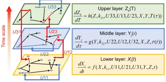
Recent improvements in high-throughput biotechnologies such as microarray [1] and mass spectrometry [2] have led to various omics data showing gene expression, protein synthesis, metabolome flux, and cell-cell interactions [3][4][5]. The ensuing accumu-lation of omics data has contributed significantly to mathematical models that indicate dynamic characteristics of biological systems, including interactions between genes, proteins, cells, and tissues [6][7] (Figure 1). Systems biology approaches such as ma-thematical modeling of multiple layers have revealed complex relationships among bi-ological phenomena of varying spatiotemporal scales, and have elucidated mechanisms with high order functions in biological systems [8] [9] [10] [11] [12]. In particular, multi-time-scale models have been applied to analyses of intracellular signal transduc-tion systems such as cell cycle control, cell fate determinatransduc-tion, and immune system mechanisms [13] [14] [15] [16]. Moreover, mathematical analyses of varying (layer) gene (seconds), metabolism (minutes), and cell (hours) transition rates in biological systems define differences between biological systems and offer important discoveries of disease mechanisms. However, efficient techniques for numerical calculations re-main elusive in practical applications of multi-time-scale mathematical models.
[image:2.595.234.514.512.651.2]Multi-time-scale models comprise multiple layers that differ in rates of state change. During conventional numerical calculations of multi-time-scale models, time step sizes that are suitable for the smallest time-scale layer have been adopted for all layers to en-sure stability and maintain calculation accuracy. Thus, dynamic behaviors of entire layers are numerically analyzed using excessively reduced time step sizes, leading to
Figure 1. Overview of the multi-time-scale model; This model has three layers and has reactions across layers. The parameters X Y Z, , indicate
concentra-tions; Uxy indicates the control variables from layer x to layer y; knn
significant increases in computational demands (time stiff problem) [17] [18] [19]. Numerous implicit methods such as the Radau method [19] and Gear method [20]
have been proposed as candidate solutions to the time stiff problem. These methods generate numerical solutions based on calculation sensitivities and stabilities of com-ponents in 1 layer. Furthermore, the numerical solutions of these methods are calcu-lated using non-linear simultaneous equations with n unknowns based on n compo-nents in the model. In calculating multi-time-scale model using the implicit method, larger time step sizes than those for the smallest time-scale layer can be applied to nu-merical calculations of all layers because the calculation stability of the implicit method is very high. However, because multi-time-scale models comprise large numbers of components, non-linear simultaneous equations that are calculated using implicit me-thods become very large. Specifically, although implicit meme-thods suppress increases in computational loads due to excessive reductions in adaptive step sizes, significant in-creases in volumes of numerical calculations for non-linear simultaneous equations cause failure to eliminate the time stiff problem. Parallel computing with reduced computational cost has been applied to numerical calculations of multi-time-scale models [21] [22] [23]. In contrast, contributions of parallel computing have been li-mited because analyses of dynamic behaviors of biological systems include numerous sequential calculations. These observations imply that the efficiency of numerical cal-culations in multi-time-scale models is highly dependent on reduced computational loads. Therefore, application of suitable step sizes to numerical calculations for each time scale layer will likely reduce computational loads significantly. Currently, few me-thods are available for determining suitable step sizes for numerical calculations of each layer in multi-time-scale models with interactions among layers, and solutions to this problem are essential for practical applications of multi-time-scale models to biological systems.
In this study, we developed a method for dynamically determining appropriate step sizes for the largest time-scale layer based on state changes of the smallest time-scale layer in numerical analysis of multi-time-scale models with interactions among layers. Subsequently, we proposed a numerical method for reducing computational loads of multi-time-scale models (proposed method) and verified the effectiveness of the pro-posed method using the follow steps:
1) Construction of multi-time-scale model (benchmark model) with interactions among layers that are universally observed in biological systems;
2) Numerical calculation of benchmark models using the conventional method (Control);
3) Numerical calculation of a benchmark model using the proposed method; 4) Comparison of computational loads for proposed and conventional methods; 5) Comparison of numerical solutions for proposed and conventional methods; 6) Discussion of the validity of the proposed method.
time-scale models with interactions among layers. By reducing computational loads, the proposed method enhances the feasibility of mathematical analyses and accommo-dates greater scales of mathematical models, representing a significant contribution to systems biology methods.
2. Material and Methods
2.1. Benchmark Models with Multi-Time-Scales
To design and develop a method that is suitable for multi-time-scale models, we con-structed 2 benchmark models (model A and model B) with the time stiff problem (Figure 2) and evaluated the calculation performance of the proposed method. The time stiff problem occurred due to differences in time-scales of each layer by interac-tions among layers. Thus, these benchmark models satisfied the following condiinterac-tions: 1) Models included interactions across layers; 2) Models had different time-scales of each layer. Models A and B comprised lower, middle, and upper layers with time scales of seconds, minutes, and hours, respectively. Model A contained inhibition effects such as suppressed expression of anabolic enzymes by metabolic products [24] and negative control of gene expression by the lac repressor protein [25], and these inhibition effects from upper to lower layers induced the time stiff problem with differences in time- scales of each layer caused by the largest time-scale layer (Figure 2(a)). Model B con-tained activation effects such as the transcriptional control by RNA polymerase [26]
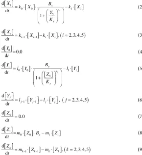
and the control of metabolic flux by enzymes [27], and these activation effects from lower to upper layers induced the time stiff problem with differences in time-scales of each layer caused by the smallest time-scale layer (Figure 2(b)). Furthermore, these ef-fects of activation and inhibition were expressed using the Hill equation [28], which empirically explains cooperative effects of oxygen binding to hemoglobin. Equations (1)-(9) show mass balance equations of model A as follows:
[ ]
0d
0.0 d
X
[image:4.595.199.548.470.663.2]t = (1)
[ ]
1[ ]
[ ]
0 0 1 1
5 d d 1 x x n x X B
k X k X
t Y K = ⋅ ⋅ − ⋅ + (2)
[ ]
[
]
[ ]
(
)
1 1 d, 2, 3, 4, 5 d
i
i i i i
X
k X k X i
t = − ⋅ − − ⋅ = (3)
[ ]
0d
0.0 d
Y
t = (4)
[ ]
[ ]
[ ]
5[ ]
1
0 0 1 1
d – d 1 y y n y B Y
l Y l Y
t K Z = ⋅ ⋅ ⋅ + (5)
(
)
1 1 d, 2, 3, 4, 5 d
j
j j j j
Y
l Y l Y j
t − −
= ⋅ − ⋅ =
(6)
[ ]
0d
0.0 d
Z
t = (7)
[ ]
1[ ]
[ ]
0 0 1 1
d
–
d z
Z
m Z B m Z
t = ⋅ ⋅ ⋅ (8)
[ ]
[
]
[ ]
(
)
1 1
d
, 2, 3, 4, 5 d
k
k k k k
Z
m Z m Z k
t = − ⋅ − − ⋅ = (9)
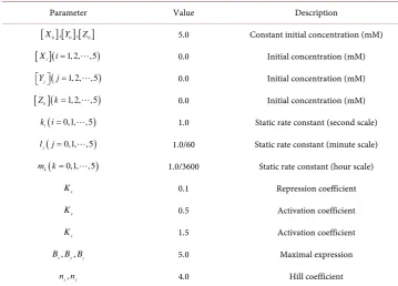
[image:5.595.258.549.72.389.2]Here, Equations (1)-(3), (4)-(6), and (7)-(9) show magnitudes of change in lower, middle, and upper layers of model A, respectively. Table 1 shows kinetic parameters of Equations (1)-(9), and Equations (10)-(18) show mass balance equations of model B as follows:
Table 1. Constants and parameters in model A.
Parameter Value Description
[ ] [ ] [ ]X0 ,Y0 , Z0 5.0 Constant initial concentration (mM) [ ]Xi (i=1, 2,, 5) 0.0 Initial concentration (mM)
( 1, 2, , 5)
j
Y j=
0.0 Initial concentration (mM)
[ ]Zk (k=1, 2,, 5) 0.0 Initial concentration (mM)
( 0,1, , 5)
i
k i= 1.0 Static rate constant (second scale)
( 0,1, , 5)
j
l j= 1.0/60 Static rate constant (minute scale)
( 0,1, , 5)
k
m k= 1.0/3600 Static rate constant (hour scale)
,
x y
K K 2.5 Repression coefficient
, ,
x y z
B B B 5.0 Maximal expression
,
x y
[ ]
0 d0.0 d
X
t = (10)
[ ]
[ ]
[ ]
[ ]
1
0 0 1 1
5 d – d 1 x x n x X B
k X k X
t X K = ⋅ ⋅ ⋅ + (11)
[ ]
[
]
[ ]
(
)
1 1 d, 2, 3, 4, 5 d
i
i i i i
X
k X k X i
t = − ⋅ − − ⋅ = (12)
[ ]
0 d0.0 d
Y
t = (13)
[ ]
[ ]
[ ]
[ ]
(
)
[ ]
1
0 0 1 1
5 5 d – d y y y n y n n y X K X B Y
l Y l Y
t
⋅
= ⋅ ⋅ ⋅
+ (14)
(
)
1 1
d
, 2, 3, 4, 5 d
j
j j j j
Y
l Y l Y j
t − −
= ⋅ − ⋅ =
(15)
[ ]
0d
0.0 d
Z
t = (16)
[ ]
[ ]
[ ]
[ ]
(
5)
[ ]
10 0 1 1
5 d – d z z z n z z n n Y K Y B Z
m Z m Z
t
⋅
= ⋅ ⋅ ⋅
+ (17)
[ ]
[
]
[ ]
(
)
1 1
d
2, 3, 4, 5 d
k
k k k k
Z
m Z m Z k
t = − ⋅ − − ⋅ = (18)
Here, Equations (10)-(12), (13)-(15), and (16)-(18) show magnitudes of change in lower, middle, and upper layers of model B. Table 2 shows kinetic parameters of Equa-tions (10)-(18). Normally, the time stiff problem occurs due to differences in time- scales of each component by dynamically changing reaction rates
(
k l mi, ,j k)
in modelA and B. In this paper, reaction rates were constant in entire time, to focus on the time difference between layers.
2.2. Numerical Solutions of the Benchmark Model Based on the Conventional Method
[image:6.595.249.548.70.410.2]We obtained numerical solutions of benchmark models (Model A, Model B) shown in
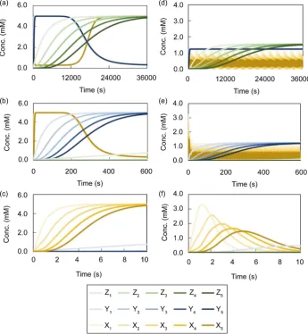
Figure 2 using the explicit 4 stage 4th-order Runge-Kutta method [29] as the conven-tional method. The simulation time was set at 36000 s because the dynamic behavior of the upper layer reached steady state at this time. The adaptive time step size dt of the
conventional method was set to 1.00E−03 s. Figures 3(a)-(c) and Figures 3(d)-(f)
show time-dependent changes of component concentrations in models A and B, re-spectively. Moreover, Figure 3(a) and Figure 3(d), Figure 3(b) and Figure 3(e), and
Table 2. Constants and parameters in model B.
Parameter Value Description
[ ] [ ] [ ]X0 ,Y0 , Z0 5.0 Constant initial concentration (mM) [ ]Xi (i=1, 2,, 5) 0.0 Initial concentration (mM)
( 1, 2, , 5)
j
Y j=
0.0 Initial concentration (mM)
[ ]Zk (k=1, 2,, 5) 0.0 Initial concentration (mM)
( 0,1, , 5)
i
k i= 1.0 Static rate constant (second scale)
( 0,1, , 5)
j
l j= 1.0/60 Static rate constant (minute scale)
( 0,1, , 5)
k
m k= 1.0/3600 Static rate constant (hour scale)
x
K 0.1 Repression coefficient
y
K 0.5 Activation coefficient
z
K 1.5 Activation coefficient
, ,
x y z
B B B 5.0 Maximal expression
,
x y
n n 4.0 Hill coefficient
upper layers were observed in time-scales of seconds, minutes, and hours, respectively. To verify calculation performance of the proposed method, we defined the results of these calculations as controls.
2.3. Design and Development of Proposed Method
In numerical calculations of the conventional method in multi-time-scale models, the adaptive time step size of the smallest time-scale layer (lower layer) was adopted in cal-culations for all layers. Hence, numbers of calculation steps of middle and upper layers were equal to that of the lower layer in the conventional method. Here we defined the process of calculating the concentration S t
(
+ ∆t)
of component S at the time t+ ∆tfrom the concentration S t
( )
of component S at time t as 1 unit of the calculation (1step), and ∆t was the adaptive time step size. Adaptive time step sizes of middle and
upper layers in the conventional method were generally much smaller than suitable for these layers. Use of optimal step sizes for middle and upper layers in numerical calcula-tions reduced the numbers of calculation steps for middle and upper layers. Therefore, we developed effective numerical calculation algorithms (proposed method) that opti-mally controlled adaptive time step sizes for each layer based on variations of differen-tial component values.
Figure 3. Time course of numerical solutions by the conventional method; The calculation step size dt of the conventional method was set to 1.00E−03 s. (a), (b), and (c) show results of the models A, (d), and (e), and (f) shows the result of model B. Simulation times of (a) and (d) were set to 36,000 s (10 h), those of (b) and (e) were set to 600 s (10 min), and those of (c) and (f) were set to 10 s.
of the arbitrary number of the Nx step, which was set to a predetermined calculation
interval. Secondly, the backward algorithm was used to define a predetermined calcula-tion interval in which the differential value was less than a certain value according to the determined calculation interval. Here, the adaptive time step size of the middle layer and the representative value for the lower layer were set to determine the calcula-tion interval and its average integral value of the numerical solucalcula-tion for the lower layer. Subsequently, the cumulative algorithm was used to calculate the dynamics of the 1st
method were fewer than those of the conventional method, reflecting differing step siz-es of proposed and conventional methods. In addition, adaptive time step sizsiz-es of mid-dle and upper layers of the proposed method were controlled by the backward algo-rithm to maintain calculation accuracy. Accordingly, the computational volume of the proposed method was less than that of the conventional method and the calculation accuracies of proposed and conventional methods were comparable. Numerical calcu-lations of the proposed method in the multi-time-scale models comprising the 3 layers of models A and B are described by Equations (19)-(21), which are mass balance equa-tions and targets of the proposed method as follows:
(
)
d
, , , d
k k Z
h X Y Z t
t = (19)
(
)
d
, , , d
j j
Y
g X Y Z t
t = (20)
(
)
d
, , , d
i i X
f X Y Z t
t = (21)
Equations (22) and (23) describe initial conditions as follows:
(
X Y Z t, , ,)
=(
X t(
=t0) (
,Y t=t0) (
,Z t=t0)
,t0)
(22)0 0 0
t =τ =T (23)
Here, the parameters X Y Z, , indicate concentration of components i j k, ,
identi-fied in each layer t, ,τ T of lower, middle and upper layer.
2.3.1. Ahead Algorithm
Initially, numbers of predetermined calculation steps
(
Nx,Ny,Nz)
were set to 60(Table 3). In the ahead algorithm, the arbitrary conventional method was adopted (Eu-ler method [29], Runge-Kutta method [29], Runge-Kutta-Fehlberg method [30] etc.) with the numerical calculation of the smallest time-scale layer (lower layer), and the iterative numerical integration in the interval of the number of Nx steps
[image:9.595.192.542.569.701.2](predeter-mined calculation interval) was implemented. The numerical calculation from the ini-tial state to the Nx step was explicitly calculated based on Equations (24) and (25) as
Table 3. Parameters of the proposed method.
Parameter Value Description
x
N 60.0 Initial number of predetermined calculation step in lower layer
y
N 60.0 Initial number of predetermined calculation step in middle layer
z
N 60.0 Initial number of predetermined calculation step in upper layer
x
A 5.0 Control variable of number of predetermined calculation step in lower layer
y
A 5.0 Control variable of number of predetermined calculation step in middle layer
z
follows:
(
)
(
)
(
(
)
(
) (
)
)
(
)
1 , 0 , 0 , d
0,1, 2, , 1
p p p p p
x
X t t X t t f X t t Y t t Z t t t t
p N
+
= = = + = = = ⋅
= − (24)
(
)
1 d 0,1, 2, , 1
p p p x
t + =t + t p= N − (25)
Here, dtp indicates the adaptive time step size per step in the lower layer, equations
for middle and upper layers were shown in Equation (36) and (46), respectively.
2.3.2. Backward Algorithm
The backward algorithm was used to explore the predetermined calculation interval in which the differential value was less than a certain value according to the determined calculation interval. Here, the number of calculation steps was set to the number of de-termined calculation steps Gx. Consequently, the backward algorithm could be used to
monitor magnitudes of change in the numerical solution of dependent variables in the predetermined calculation interval. Subsequently, the backward algorithm narrowed the determined calculation interval for large changes in numerical solutions of the de-pendent variable in the predetermined calculation interval and widened that when changes were small. To measure magnitudes of change of all components in the layer, we compared the final differential value Dx_ 2 of each component at the time tNx
with the average integral value f of the differential value in the predetermined
calcu-lation interval using Equation (26) as follows:
_ 2 x
E= f −D (26)
Here, E is evaluation value of each component in the predetermined calculation in-terval and this evaluation value shows the magnitude of change in the differential value of each component during the predetermined calculation interval. Using Simpson’s numerical integration method [29] to the coordinate points
(
C D,)
of time and thedifferential value, we determined the average integral value f of the differential value
in the predetermined calculation interval. Equations (27)-(29) show the coordinate points
(
C D,)
of time and the differential value as follows:(
Cx_ 0,Dx_ 0)
=(
t0,f X t(
(
=t0) (
,Y t=t0) (
,Z t=t0)
,t0)
)
(27)(
Cx_1,Dx_1)
=(
t f X t1,(
(
=t1) (
,Y t=t0) (
,Z t=t0)
,t1)
)
(28)(
Cx_ 2,Dx_ 2)
=(
tNx,f X t(
(
=tNx)
,Y t(
=t0) (
,Z t=t0)
,tNx)
)
(29) We obtained differential values Dx M_ at the midpoint of the predeterminedcalcu-lation interval Cx M_ =
(
Cx_ 2−Cx_ 0)
2 using the Lagrange interpolation [29] asshown in Equations (30) and (31) as follows:
(
)
2
_ _ _
0
x M u x M x u
u
D L C D
=
(
)
2( )_ _
_
0 _ _
v u
x M x v u x M
v x u x v
C C L C C C ≠ = − = −
∏
(31)The average integral value f was calculated using the coordinate points
(
C D,)
and the differential value Dx_ 2 (Equation (32)) as follows:
(
)
(
) (
)
_ 2
_ 0
_ 2 _ 0
_ 2 _ 0
_ 0 _ _ 2
_ 2 _ 0
_ 0 _ _ 2
, , , d
4 6 4 6 x x t C t C x x x x
x x M x
x x
x x M x
f X Y Z t t f
C C
C C
D D D
C C
D D D
= = = − − ⋅ + + = − + + =
∫
(32)Evaluation value E (Equation (26)) was calculated as the average integral value f
and the differential value Dx_ 2. We determined the dependent variable of the lower
layer when evaluation value E of all components in the lower layer were less than or equal to the threshold value (α) (E ≤ α). However, we updated the coordinate points
(
Cx_ 2,Dx_ 2)
to Equation (33) and calculated the Dx M_ , f and evaluation value Ewhen at least one of E were greater than the threshold value (α) (E > α) as follows:
(
)
(
(
(
)
(
) (
)
)
)
(
)
_ 2 _ 2 0 0
x
, , , , ,
1, 2, 3, , 2
x x x x x x
x x N S N S N S
x
C D t f X t t Y t t Z t t t
S N
− − −
= = = =
= − (33)
Thereafter, we sequentially increased the number of discarded calculation steps Sx
until E of all components in the lower layer were less than or equal to the threshold value (α) (E ≤ α) and determined the dependent variable of the lower layer. The num-ber of determined calculation steps Gx was set to Nx−Sx when the all evaluation
values E were less than or equal to the threshold value (α) (Equation (34)) as follows:
x x x
G =N −S (34)
If E was more than the threshold value (α) at Sx =Nx−2, we set it to Gx =2.
Equ-ation (35) shows the coordinate points
(
Cx_ 2,Dx_ 2)
after the number of determinedcalculation steps Gx was decided as follows:
(
Cx_ 2,Dx_ 2)
=(
tGx,f X t(
(
=tGx)
,Y t(
=t0) (
,Z t=t0)
,tGx)
)
(35)2.3.3. Cumulative Algorithm
After determining the calculation interval of the lower layer with the backward algo-rithm, the cumulative algorithm was used to implement the numerical calculation of the 1st step in the middle layer using Equations (36)-(39) as follows:
(
1)
(
0)
(
,(
0) (
, 0)
, 0)
d 0( )
(
) (
(
)
(
) (
)
)
(
)
(
) (
)
_ 2
_ 0
_ 2 _ 0
_ 2 _ 0
_ 0 _ _ 2
_ 2 _ 0
_ 0 _ _ 2
d 4 6 4 6 x x t C t C x x x x
x x M x
x x
x x M x
X t t X
C C
C C
X t C X t C X t C
C C
X t C X t C X t C
= = = − − ⋅ = + = + = = − = + = + = =
∫
(37) 10 _ 2 _ 0
0
d d
x
G
x x j
j
C C t
τ −
=
= − =
∑
(38)(
)
1 d , 0,1, 2, , 1
q q q q Ny
τ + =τ + τ = − (39)
Here, dτ0 was equal to the interval from time Cx_ 0 to time Cx_ 2 and X was
the time-averaged concentration of the numerical solution of the lower layer in the in-terval from time Cx_ 0 to time Cx_ 2. In addition, X t
(
=Cx M_)
was calculated usingLagrange interpolation [29]. We applied the conventional method shown in the ahead algorithm to the numerical calculation of the middle layer.
2.3.4. Integration of Whole Algorithms
Calculations of these algorithms gave numerical solutions of lower and middle layers at time τ1. Subsequently, the numerical solution of the concentration of the component
in the interval from the
(
Gx+1)
step to the(
Gx+Nx)
step in the lower layer (thepredetermined calculation interval) was calculated using the ahead algorithm with the values X t
(
=τ1)
and Y t(
=τ1)
as shown in Equation (40) as follows:(
)
(
)
(
(
)
(
) (
)
)
(
)
1 1
1 1 , 1 , 0 , 1 d
0,1, 2, , 1 p
p p p p
x X t t
X t t f X t t Y t Z t t t t
p N
τ
τ τ τ τ
+
= +
= = + + = + = = + ⋅
= −
(40)
Thereafter, the backward algorithm was used to define the number of determined calculation steps Gx and the number of discarded calculation steps Sx in this
pre-determined calculation interval, and the cumulative algorithm was used to calculate
(
2)
Y t=τ of the middle layer. We repeated the procedures in Equations (26)-(40), and
the numerical solution of the component concentration of the middle layer was calcu-lated until the Ny step (the predetermined calculation interval in the middle layer)
using the following Equations (41) and (42):
(
)
(
)
(
(
)
(
)
)
(
)
1
0
, , , d
0,1, 2, , 1 q
q q q q
y Y t
Y t g X Y t Z t
q N
τ
τ τ τ τ τ
( )
(
)
(
)
(
)
(
)
(
)
1 1 1 1 1 1 1 1 d 4 6 2 4 2 6 q q t t q qq q q q
q q
q q
q q
q q
X t t X
X t X t X t
X t X t X t
τ τ
τ τ
τ τ τ τ
τ τ τ τ τ τ τ τ + = = + + + + + + + ′ = − − − ⋅ = + = + = = − − = + = + = =
∫
(42)Here, X′ denotes the time-averaged concentration of the numerical solution of the
lower layer in the interval from time τq to τq+1. The number of determined
calcula-tion steps Gy was then decided and the number of discarded calculation steps Sy in
middle layer was generated using the backward algorithm. Equations (43)-(45) show the coordinate points of the differential value and the time of the middle layer that is necessary for the corresponding calculation of E (Equation (26)) as follows:
(
Cy_ 0,Dy_ 0)
=(
τ0,g X t(
(
=τ0) (
,Y t=τ0) (
,Z t=τ0)
,τ0)
)
(43)(
Cy_1,Dy_1)
=(
τ1,g X t(
(
=τ1) (
,Y t=τ1) (
,Z t=τ0)
,τ1)
)
(44)(
Cy_ 2,Dy_ 2)
=(
τGy,g X t(
(
=τGy) (
,Y t=τGy)
,Z t(
=τ τ0)
, Gy)
)
(45)The cumulative algorithm was used to implement the calculation of the 1st step of the upper layer with numerical solutions of lower and middle layers using Equations (46)-(50) as follows:
(
1)
(
0)
(
, ,(
0)
, 0)
d 0Z t=T =Z t=T +h X Y Z t′′ =T T ⋅ T (46)
( )
(
)
(
(
)
(
)
)
(
)
(
) (
)
_ 2 _ 0
_ 2 _ 0
_ 2 _ 0
_ 0 _ _ 2
_ 2 _ 0
_ 0 _ _ 2
d 4 ( 6 4 6 y y t C t C y y y y
y y M y
y y
y y M y
X t t X
C C
C C
X t C X t C X t C
C C
X t C X t C X t C
= = ′′ = − − ⋅ = + = + = = − = + = + = =
∫
(47)( )
(
) (
(
)
(
) (
)
)
(
)
(
) (
)
_ 2 _ 0_ 2 _ 0
_ 2 _ 0
_ 0 _ _ 2
_ 2 _ 0
_ 0 _ _ 2
d 4 6 4 6 y y t C t C y y y y
y y M y
y y
y y M y
Y t t Y
C C
C C
Y t C Y t C Y t C
C C
Y t C Y t C Y t C
1
0 _ 2 _ 0 0
d d
y
G
y y j
j
T C C τ
−
=
= − =
∑
(49)(
)
1 d 0,1, 2, , 1
r r r z
T+ =T + T r= N − (50)
Here, dT0 was equal to the interval from the time Cy_ 0 to the time Cy_ 2, and X′′ was the corresponding time-averaged concentration of the numerical solution of
the lower layer. Y was the time-averaged concentration of the numerical solution of
the middle layer in the same time interval and X t
(
=Cy M_)
and Y t(
=Cy M_)
werecalculated using Lagrange interpolation [29]. The numerical calculation of the upper layer shown in Equation (46) applied the same conventional method in the case of the ahead algorithm (Equation (24)). Subsequently, we repeated Equations (26)-(50) and found the numerical solution from t=T0 to t=TNz of the dependent variable in the
upper layer. Finally, the backward algorithm was used to define the number of deter-mined calculation steps Gz and the number of discarded calculation steps Sz in the
upper layer. After completion of upper layer calculations, we calculated iterative nu-merical integrations in the interval of Nx steps of the lower layer using the values
(
Gz)
X t=T ,
(
)
z
G
Y t=T and
(
)
z
G
Z t=T in Equation (51) as follows:
(
)
(
)
(
(
) (
) (
)
)
(
)
1
, , , d
0,1, 2, , 1
z
z z z z z
p G
p G p G G G p G p
x
X t t T
X t t T f X t t T Y t T Z t T t T t
p N
+
= +
= = + + = + = = + ⋅
= −
(51)
Iterative calculations of component concentrations of all layers were calculated using Equations (26)-(51).
2.3.5. Control of Numbers of Predetermined Calculation Steps
Numbers of predetermined calculation steps
(
Nx,Ny,Nz)
indicated numbers ofcal-culations with the ahead algorithm. When numbers of predetermined calculation steps
(
Nx,Ny,Nz)
were excessively large, the backward algorithm discarded the calculationobtained by the ahead algorithm to maintain calculation accuracy. Therefore, the number of predetermined calculation steps
(
Nx,Ny,Nz)
was closely related to thecalculation efficiency of the proposed method, and the number of predetermined cal-culation steps
(
Nx,Ny,Nz)
was dynamically changed based on the number ofdeter-mined calculation steps as shown in Equation (52) as follows:
x x x
y y y
z z z
N G A
N G A
N G A
= +
(52)
Here, A A Ax, y, z were increments of the number of predetermined calculation steps
(
Nx,Ny,Nz)
. Accordingly, Equation (52) implicitly controlled the number of2.4. Evaluation of Calculation Accuracy
The calculation accuracy of the proposed method was evaluated using Equations (53) and (54). Firstly, we evaluated calculation accuracy according to the consistency of the numerical solution using Equation (53) as follows:
_
1 _
1 num
a proposed method ave
a a conventional method
Component V
num = Component
=
∑
(53)where Componenta_proposed method and Componenta conventional method_ were corresponding
to the numerical solution of specific Componenta
(
a=1, 2, 3,,num)
in the layer ofinterest using the proposed and conventional method, respectively. The num represented the number of components in the layer of interest. The right side of Equa-tion (53) was the average of proporEqua-tion of the numerical soluEqua-tion from the proposed method
(
Componenta_proposed method)
to that of the conventional method(
Componenta conventional method_)
. Secondly, we evaluated local calculation accuracyac-cording to the standard deviation of the value between the numerical solution of the proposed method and that of the conventional method using Equation (54) as follows:
2 _
1 _
1 num
a proposed method
SD ave
a a conventional method Component
V V
num = Component
= −
∑
(54)Hence, calculation accuracy was evaluated according to Vave and VSD.
3. Results
In the multi-time-scale models (Model A, Model B) shown in Figure 2, we compared numerical solutions of the proposed method with those of the conventional method. In the conventional method, we adopted the explicit 4 stage 4th-order Runge-Kutta me-thod [29] for numerical calculations of all layers. However, the numerical calculation of the lower layer of the proposed method allowed application of the arbitrary method for ordinary differential equations. We also adopted the explicit 4 stage 4th-order Runge- Kutta method [29] for the numerical calculations of the lower layer of the proposed method. Table 1 and Table 2 show kinetic parameters of models A and B, respectively, and the simulation time was set to 36000 s because the dynamic behavior of the upper layer reached steady state at this time. The step size dt of the adaptive time of the expli-cit 4 stage 4th-order Runge-Kutta method [29] was used in the proposed method and the conventional method, and was set to 1.00E−03 s.
3.1. Case Study 1
calcula-tion steps
(
Nx,Ny,Nz)
and parameters of control variables for numbers ofpredeter-mined calculation steps
(
A A Ax, y, z)
of the proposed method. The threshold value (α)of the evaluation value E of the backward algorithm was set to 1.00E−03, 5.00E−04, and 1.00E−04.
3.1.1. Calculation Efficiency of the Proposed Method in Numerical Analyses of Model A
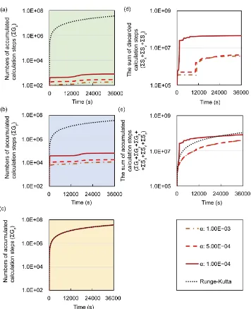
In numerical analyses of model A, the calculation efficiency of the proposed method was compared with that of the conventional method. Figures 4(a)-(c) show time- dependent changes in numbers of accumulated calculation steps for each layer in model A. Here, numbers of accumulated calculation steps for lower, middle, and upper layers were equal to the sum of Gx
(
∑
Gx)
, Gy(
∑
Gy)
and Gz(
∑
Gz)
within theen-tire simulation time for model A. We applied the same method to the numerical calcu-lation for the lower layer of the proposed and conventional methods. Hence, numbers of accumulated calculation steps for the lower layer of the proposed method was equal to that of the conventional method (Figure 4(c)). Furthermore, we compared numbers of accumulated calculation steps in middle and upper layers of model A (Figure 4(a)
and Figure 4(b)). Accumulated calculation steps in middle and upper layers of the proposed method at 36,000 s (Table 4) were far fewer than those of the conventional method in middle and upper layers of model A. Moreover, the threshold value (α) of the evaluation value E and the number of accumulated calculation steps of the pro-posed method in middle and upper layers were negatively correlated. Figure 4(d)
shows the sum of calculation steps that were discarded by the backward algorithm, which ensured calculation accuracy. In these analyses, the sum of discarded calculation steps was equal to
∑
Sx+∑
Sy+∑
Sz within the entire simulation time for model A. [image:16.595.193.554.559.707.2]Moreover, regardless of the threshold value (α), destruction of the calculation by the backward algorithm occurred during the early stages of the simulation. In addition, de-struction of calculations had occurred at 12,000 s when the threshold value (α) was 1.00E−3 or 5.00E−04. Figure 4(e) shows time-dependent changes in the sum of accu-mulated calculation steps for all layers of model A. The proposed method included the
Table 4. Calculation efficiency of the proposed method in middle and upper layers of model A at 36000 s.
Layer of the evaluation value E The threshold value (α)
Numbers of accumulated calculation steps of the conventional method (A)
Numbers of accumulated calculation steps of the proposed method (B)
Percentage ((B/A) * 100%)
Middle 1.00E−03 3.60E+07 1.13E+04 0.031
5.00E−04 3.60E+07 1.78E+04 0.049
1.00E−04 3.60E+07 6.22E+04 0.173
Upper 1.00E−03 3.60E+07 1.86E+02 0.00052
5.00E−04 3.60E+07 2.97E+02 0.00082
Figure 4. Comparisons of numbers of accumulated calculation steps for the proposed and con-ventional methods in model A; The calculation step size dt was set at 1.00E−03 s. The
thre-shold value (α) of the evaluation value E of the backward algorithm was set at 1.00E−03, 5.00E−04, and 1.00E−04. (a), (b), and (c) show the sum of numbers of accumulated calculation steps for lower, middle, and upper layers in model A
(
∑ ∑ ∑
Gx, Gy, Gz)
. (d) shows the sum of calculationsteps that were discarded by the backward algorithm in model A
(
∑
Sx+∑
Sy+∑
Sz)
. (e) showsthe sum of accumulated calculation steps of all layers in model A
(
∑
Gx+∑
Gy+∑
Gz+∑
Sx+∑
Sy+∑
Sz)
.sum of calculation step that were discarded by the backward algorithm as
x y z x y z
G + G + G + S + S + S
∑
∑
∑
∑
∑
∑
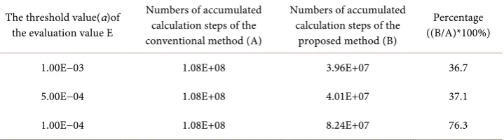
. Accumulated calculation steps of the pro-Table 5. Calculation efficiency of the proposed method in all layers of model A at 36000 s.
The threshold value(α)of the evaluation value E
Numbers of accumulated calculation steps of the conventional method (A)
Numbers of accumulated calculation steps of the proposed method (B)
Percentage ((B/A)*100%)
1.00E−03 1.08E+08 3.96E+07 36.7
5.00E−04 1.08E+08 4.01E+07 37.1
1.00E−04 1.08E+08 8.24E+07 76.3
lation steps) were greater than those that were discarded by the backward algorithm (increased numbers of calculation steps), which was dependent on the threshold value (α), the sum of accumulated calculation steps for all layers of the proposed method was reduced.
3.1.2. Calculation Accuracy of Proposed Method in Numerical Analysis of Model A
The numerical solution of the proposed method was compared with that of the conven-tional method in model A. Figures 5(a)-(c) show time-dependent changes of the eval-uation value Vave (Equation (53)), which represents consistency of the numerical
solu-tion. Figures 5(d)-(f) show time-dependent changes of the evaluation value VSD
(Eq-uation (54)), which represents local calculation accuracy. In any layer, Vave was within
the range of 0.95 - 1.05 and VSD was 0.01 or less at all times. Moreover, Vave was
asymptotic to 1.0 with decreases in thresholds (α) of the evaluation value E in all layers. Therefore, the calculation accuracy of the proposed method was almost the same as that of the conventional method in numerical analyses of model A.
3.2. Case Study 2
As shown in Figure 2(b), model B comprised 18 components and had activation effects from lower to middle layers and from middle to upper layers. In addition, the effect of negative feedback in the lower layer led to oscillating dynamics in model B. In the pre- sent study, we compared numerical solutions of the proposed and conventional me-thods in model B and verified the utility of the proposed method in the multi- time-scale model in terms of calculation efficiencies and accuracies. Table 3 shows pa-rameters of initial numbers of predetermined calculation steps
(
N Nx, y,Nz)
andpa-rameters of control variables for numbers of predetermined calculation steps
(
A A Ax, y, z)
of the proposed method. Threshold values (α) of the evaluation value E ofthe backward algorithm were set at 1.00E−01, 5.00E−02, and 1.00E−02.
3.2.1. Calculation Efficiency of the Proposed Method in Numerical Analyses of Model B
Figure 5. Comparison of calculation accuracies of the proposed and conventional methods in model A; Vertical axes of (a), (b), and (c) show Vave (Equation (53)). Vertical axes of (d), (e),
and (f) show VSD (Equation (54)). The threshold value (α) of the evaluation value E of the back-
ward algorithm was set at 1.00E−03, 5.00E−04, and 1.00E−04.
Figure 6. Comparison of numbers of accumulated calculation steps for proposed and conven-tional methods in model B; The calculation step size dt was set at 1.00E−03. The threshold value (α) of the evaluation value E for the backward algorithm was set at 1.00E−01, 5.00E−02, and 1.00E−02. (a), (b), and (c) show the sum of accumulated calculation steps for lower, middle, and upper layers in model B
(
∑ ∑ ∑
Gx, Gy, Gz)
. (d) shows the sum of calculation steps that werediscarded by the backward algorithm in model B
(
∑
Sx+∑
Sy+∑
Sz)
. (e) shows the sum ofaccumulated calculation steps for all layers in model B
(
∑
Gx+∑
Gy+∑
Gz+∑
Sx+∑
Sy+∑
Sz)
.lay-ers of model B (Figure 6(a) and Figure 6(b)). Table 6 shows numbers of accumulated calculation steps in middle and upper layers of the proposed method at 36000 s in model B relative to those of the conventional method. Numbers of accumulated calcu-lation steps for the proposed method were far fewer than those of conventional method in middle and upper layers of model B. Moreover, threshold values (α) of E from the backward algorithm were negatively correlated with numbers of accumulated calcula-tion steps of the proposed method in middle and upper layers. Figure 6(d) shows the sum of calculation steps that were discarded by the backward algorithm, which was used to ensure calculation accuracy. In these analyses, the sum of discarded calculation steps was equal to
∑
Sx+∑
Sy+∑
Sz within the entire simulation time for model B.In case study 2, the calculation was discarded at a constant rate with time. Figure 6(e)
[image:21.595.194.554.431.568.2] [image:21.595.195.556.603.701.2]shows time-dependent changes of the sum of accumulated calculation steps for all lay-ers in model B. The proposed method included the sum of calculation steps that were discarded by the backward algorithm as
∑
Gx+∑
Gy+∑
Gz+∑
Sx+∑
Sy+∑
Sz. Table 7 shows the sum of accumulated calculation steps for all layers of proposed me-thod at 36000 s in model B as a proportion of that for the conventional meme-thod. In case study 2, decreases in numbers of accumulated calculation steps in middle and upper layers of the proposed method were greater than the increases in numbers of calcula-tion steps that were discarded by the backward algorithm, which was dependent on the threshold value (α). Thus, the sum of accumulated calculation steps of all layers of the proposed method was reduced.Table 6. Calculation efficiency of the proposed method in middle and upper layers of model B at 36,000 s.
Layer (The threshold value α) of the evaluation value E
Numbers of accumulated calculation steps of the conventional method (A)
Numbers of accumulated calculation steps of the
proposed method (B)
Percentage ((B/A) * 100%)
Middle 1.00E−01 3.60E+07 1.67E+05 0.464
5.00E−02 3.60E+07 2.31E+05 0.642
1.00E−02 3.60E+07 7.09E+05 1.970
Upper 1.00E−01 3.60E+07 1.39E+03 0.0039
5.00E−02 3.60E+07 2.82E+03 0.0078
1.00E−02 3.60E+07 1.88E+04 0.0522
Table 7. Calculation efficiency of the proposed method in all layers of model B at 36,000 s.
The threshold value(α)of the evaluation value E
Numbers of accumulated calculation steps of the conventional method (A)
Numbers of accumulated calculation steps of the proposed method (B)
Percentage ((B/A) * 100%)
1.00E−01 1.08E+08 3.86E+07 35.7
5.00E−02 1.08E+08 3.96E+07 36.7
3.2.2. Calculation Accuracy of the Proposed Method for Numerical Analysis of Model B
The numerical solution of proposed method was compared with that of the conven-tional method in model B. Figures 7(a)-(c) show time-dependent changes in the eval-uation value Vave (Equation (53)), which represents consistency of the numerical
solu-tion, and Figures 7(d)-(f) show time-dependent changes of the evaluation value VSD
(Equation (54)), which represents local calculation accuracy. In any layer, Vave was
within the range of 0.99 - 1.01, and VSD was 0.01 or less at all times. Therefore, the
calculation accuracy of the proposed method was almost the same as that of the con-ventional method in numerical analyses of model B.
4. Discussion
The advent of high-throughput experimental devices that can accommodate large numbers of samples has allowed simultaneous computation of comprehensive data pertaining to genome, transcriptome, proteome, and metabolome analyses [1][2][3][4] [5]. Consequently, the momentum of theoretical analyses of biological systems that use multi-time-scale models is growing [13][14] [15] [16] (Figure 1). In theoretical ana-lyses of multi-time-scale models with reactions between layers, the time stiff problem
[17][18][19] occurs due to differences in time-scales of each layer, leading to signifi-cant increases in computation times. In particular, the time stiff problem signifisignifi-cantly influences the efficiency of numerical optimizations of system identifications and ana-lyses. Optimization methods are generally used to search for optimum solutions using repeated calculations with varying kinetic parameters for different strategies. For ex-ample, system identification by the Real-coded Genetic Algorithm (AREX + JGG) re-quired about 2.0E+06 calculation iterations to estimation parameter values for 112 ele-ments [31]. Calculation times for numerical optimization are generated by multiplying numbers of calculations by the time taken for 1 calculation. Because the time taken for 1 calculation is greatly increased by time stiff problems, calculation times for numerical optimizations also increase linearly. Hence, solutions for the time stiff problem will likely contribute to the efficiency of numerical optimizations. The time stiff problem also occurs in theoretical analyses of natural phenomena, such as the movements of the local clouds and typhoons in simulations of weather conditions [32] and motions and binding of compounds in simulations of chemical reactions [33]. Hence, solutions to the time stiff problem are applicable to varied mathematical analyses, including those of biological systems. In the present conventional method, the time stiff problem re-mained because the calculation of all layers was implemented by adaptive time step siz-es of the smallsiz-est time-scale layer. Therefore, the prsiz-esent alternative method reduced computation times by controlling adaptive time step sizes for each layer based on varia-tions of differential values of the components.
Figure 7. Comparison of calculation accuracies of the proposed and conventional methods in model B; Vertical axes of (a), (b), and (c) show Vave (Equation (53)). Vertical axes of (d), (e),
and (f) show VSD (Equation (54)). The threshold value (α) of the evaluation value E of the back-
ward algorithm was set at 1.00E−03, 5.00E−04, and 1.00E−04.
of change in the differential value during the predetermined calculation interval. Sub-sequently, the cumulative algorithm calculated the 1st step of the middle layer using the determined calculation interval of the lower layer and the time-averaged concentration in the determined calculation interval of the lower layer. The proposed method identi-fied numerical solutions by repeating the three algorithms for the upper layer. In the conventional method, numbers of calculation steps for middle and upper layers were equal to that of the lower layer so that all layers were calculated according to the adap-tive time step size of the lower layer. However, the adapadap-tive time step size of middle and upper layers of the proposed method were much larger than those of the conventional method. In addition, the backward algorithm narrowed the calculation interval for large changes in the numerical solution of the predetermined calculation interval and widened that in the presence of small changes. Accordingly, the proposed method sig-nificantly reduced the number of calculation steps for middle and upper layers and maintained calculation accuracy of the backward algorithm. Most current high-speed calculation methods utilize parallel computer resources [21][22][23], which are expe-dited by dividing the processing of calculations of 1 step between multiple central processing units. In contrast, the proposed method accelerates analyses by reducing numbers of calculation steps. Therefore, the proposed method does not compete with conventional high-speed methods, and can be used in conjunction with various high-speed calculation methods as a calculation module.
In the present study, we created multi-time-scale models as a benchmark (Figure 2) and verified the calculation performance of the proposed method. To this end, we in-vestigated numbers of accumulated calculation steps for each layer of proposed and conventional methods. In case studies 1 and 2, numbers of accumulated calculation steps for the lower layer were comparable in proposed and conventional methods, whereas these were fewer for middle and upper layers of the proposed method than of the conventional method (Figures 4(a)-(c), Figures 6(a)-(c)). Therefore, calculations of middle and upper layers were performed using the proposed method with optimal adaptive time step sizes.
In further analyses, we discarded calculation steps to maintain calculation accuracy in backward algorithm. In case study 1, the sum of discarded calculation steps rapidly increased between the early stages of the simulation and 12,000 s (Figure 4(d)). More-over, increasing numbers of discarded calculation steps during early stages of the simu-lation were greatly affected by initial setting values of Nx,Ny,Nz, which are
parame-ters of the proposed method. Accordingly, the ahead algorithm of the proposed method was used to calculate numerical solutions to initial setting values of Nx,Ny,Nz, and
the backward algorithm was used to discard calculations and maintain calculation ac-curacy. Therefore, the present backward algorithm significantly discarded significant numbers of calculations in the early stages of the simulation, because the initial setting values of Nx,Ny,Nz were excessive. Moreover, increasing numbers of discarded
of Y5 based on increases of Z5 and enhancements of the inhibitory effects of Z5. To
prevent the deterioration of calculation accuracy due to these variations, the backward algorithm was used to adjust the adaptive time step size for each layer to values that corresponded with magnitudes of change in numerical solutions of the dependent va-riable. Hence, the backward algorithm significantly discarded calculations by 12,000 s in case study 2. The sum of discarded calculation steps also increased linearly with time (Figure 6(d)). Because model B was of the oscillation system, destruction by the back-ward algorithm occurred in constant cycles. These analyses suggest that the backback-ward algorithm facilitates calculation accuracy.
Numbers of accumulated calculation steps of all layers of proposed and conventional methods were computed for case studies 1 and 2, and decreases by the proposed me-thod for middle and upper layers (Figure 4(a) and Figure 4(b), Figure 6(a) and Figure 6(b)) were greater than increases in those discarded by the calculation steps of the backward algorithm (Figure 4(d), Figure 6(d)). Hence, because reductions in compu-tational volumes by the proposed method were more numerous than those required to maintain calculation accuracy, the proposed method achieved the calculation efficiency of the numerical calculation in case studies 1 and 2 (Figure 4(e), Figure 6(e)).
In comparisons of calculation accuracies of proposed and conventional methods, that of the proposed method was controlled by the threshold (α) of the evaluation value E. The calculation interval that was determined by the backward algorithm was asymp-totic to predetermined calculation intervals with the increase of the threshold (α). Time step sizes of middle and upper layers also became larger. Moreover, the numerical solu-tion of the upper layer was reflected in lower and middle layers after 1 step of upper layer calculations. Thus, this reflection time was significantly delayed with excessive step sizes of the upper layer in the presence of high threshold (α) values. This delay caused calculation error in the numerical solution of the proposed method. Hence, threshold (α) values of models that contains reactions from upper to lower layers such as case study 1 need to be smaller than that in the model for case study 2. In this study, threshold (α) values of case study 1 (1.00E−03, 5.00E−04, and 1.00E−04) were set smaller than that of case study 2 (1.00E−01, 5.00E−02, 1.00E−02). Accordingly, at threshold (α) values of 1.00E−03 or 5.00E−04, calculation errors occurred in middle and upper layers for case study 1. However, at threshold (α) < 1.00E−04, calculation errors were avoided. Therefore, in case studies 1 and 2, the calculation accuracy of the conventional method was maintained by the proposed method by setting the optimal threshold (α) value depending on the model (Figure 5, Figure 7).
5. Conclusion
scale model. Accordingly, we suggest that the proposed method is an efficient numeri-cal method for multi-time-snumeri-cale models.
Acknowledgements
This work was supported by Grant-in-Aid for Scientific Research on Innovative Areas 16H01700 and Grant-in-Aid for Challenging Exploratory Research16K12912.
References
[1] Castel, D., Pitaval, A., Debily, M.A. and Gidrol, X. (2006) Cell Microarrays in Drug Discov-ery. Drug Discovery Today, 11, 13-14. https:/doi.org/10.1016/j.drudis.2006.05.015
[2] Aebersold, R. and Mann, M. (2003) Mass Spectrometry-Based Proteomics. Nature, 13, 198- 207. https:/doi.org/10.1038/nature01511
[3] Bleicher, K.H., Böhm, H.J., Müller, K. and Alanine, A.I. (2003) A Guide to Drug Discovery: Hit and Lead Generation: Beyond High-Throughput Screening. Nature Reviews Drug Dis-covery, 2, 369-378. https:/doi.org/10.1038/nrd1086
[4] Macarron, R., Banks, M.N., Bojanic, D., Burns, D.J., Cirovic, D.A., Garyantes, T., Green, D.V., Hertzberg, R.P., Janzen, W.P., Paslay, J.W., Schopfer, U. and Sittampalam, G.S. (2011) Impact of High-Throughput Screening in Biomedical Research. Nature Reviews Drug Dis-covery, 10, 188-195. https:/doi.org/10.1038/nrd3368
[5] Fischer, E., Zamboni, N. and Sauer, U. (2004) High-Throughput Metabolic Flux Analysis Based on Gas Chromatography-Mass Spectrometry Derived 13C Constraints. Analytical
Bi-ochemistry, 325, 308-316. https:/doi.org/10.1016/j.ab.2003.10.036
[6] Ge, H., Walhout, A.J. and Vidal, M. (2003) Integrating “Omic” Information: A Bridge Be-tween Genomics and Systems Biology. Trends in Genetics, 19, 551-560.
https:/doi.org/10.1016/j.tig.2003.08.009
[7] Altaf-Ul-Amin, M., Afendi, F.M., Kiboi, S.K. and Kanaya, S. (2014) Systems Biology in the Context of Big Data and Networks. BioMed Research International, 2014, Article ID: 428570. https:/doi.org/10.1155/2014/428570
[8] Hood, L. (2003) Leroy Hood Expounds the Principles, Practice and Future of Systems Bi-ology. Drug Discovery Today, 8, 436-438.
https:/doi.org/10.1016/S1359-6446(03)02710-7
[9] Kitano, H. (2002) Systems Biology: A Brief Overview. Science, 295, 1662-1664.
https:/doi.org/10.1126/science.1069492
[10] Kitano, H. (2002) Computational Systems Biology. Nature, 420, 206-210.
https:/doi.org/10.1038/nature01254
[11] Liu, E.T. (2005) Systems Biology, Integrative Biology, Predictive Biology. Cell, 121, 505- 506. https:/doi.org/10.1016/j.cell.2005.04.021
[12] Papp, B., Notebaart, R.A. and Pál, C. (2011) Systems-Biology Approaches for Predicting Genomic Evolution. Nature Reviews Genetics, 12, 591-602.
https:/doi.org/10.1038/nrg3033
[13] Yao, Z., Petschnigg, J., Ketteler, R. and Stagljar, I. (2015) Application Guide for Omics Ap-proaches to Cell Signaling. Nature Chemical Biology, 11, 387-397.
https:/doi.org/10.1038/nchembio.1809

![Figure 2 using the explicit 4 stage 4th-order Runge-Kutta method [29] as the conven-](https://thumb-us.123doks.com/thumbv2/123dok_us/7815282.730829/6.595.249.548.70.410/figure-using-explicit-stage-runge-kutta-method-conven.webp)