Strategic voting and nomination
Green-Armytage, James
UC Santa Barbara
14 April 2011
Online at
https://mpra.ub.uni-muenchen.de/32200/
Strategic Voting and Nomination
Abstract: Using computer simulations based on three separate data generating processes, I estimate the fraction of elections in which sincere voting will be a core equilibrium given each of eight single-winner voting rules. Additionally, I determine how often each voting
rule is vulnerable to simple voting strategies such as ‗burying‘ and ‗compromising‘, and how
often each voting rule gives an incentive for non-winning candidates to enter or leave races. I find that Hare is least vulnerable to strategic voting in general, whereas Borda, Coombs, approval, and range are most vulnerable. I find that plurality is most vulnerable to compromising and strategic exit (which can both reinforce two-party systems), and that Borda is most vulnerable to strategic entry. I support my key results with analytical proofs.
1. Introduction
For many who seek to improve the political process, alternative voting rules offer the possibility
of transformative change; however, there is no consensus on which rule is best. When evaluating
these systems, we must consider the extent to which they will encourage strategic behavior. I
distinguish between two basic types of election strategy: The first is strategic voting, which means
voters reporting preferences that differ from their sincere appraisal of the candidates. The second is
strategic nomination, which means non-winning candidates attempting to change the result by
entering or exiting races.
Since Gibbard (1973) and Satterthwaite (1975) demonstrated that all reasonable voting rules
create incentives for strategic voting in at least some situations,1 several authors have attempted to
assess the degree to which different voting rules are susceptible to manipulation. There is no
universally accepted way to measure this vulnerability, but one of the most common approaches has
been to estimate the fraction of elections in which manipulation is logically possible, given some
assumption about the distribution function that governs voters‘ preferences over candidates. Some
papers are concerned with the probability that an individual voter will be able to change the result to
his own benefit by voting insincerely,2 while others are concerned with the probability that a
1
Specifically, if there are more than two candidates for a single office, and a non-dictatorial election method allows voters to rank the candidates in any order, then there must be some profile of voter preferences under which at least one voter can get a preferred result by voting insincerely. This well-known ‗Gibbard-Satterthwaite theorem‘ relies in turn on the even more well-known ‗Arrow theorem‘—for this, see Arrow (1951, rev. ed. 1963).
2
For example, Nitzan (1985), Kelley (1993), Smith (1999), and Aleskerov and Kurbanov (1999). Saari (1990) focuses
coalition of voters will be able to change the result to all of its members‘ mutual benefit by voting
insincerely,3 and still others are concerned with both.4 Here, I focus on coalitional manipulation.
In this paper, I extend the literature in at least five ways. First, I produce separate results for
each of two distinct types of strategic voting –‗compromising‘ and ‗burying‘– which have different
implications for political behavior, and I show the effect of limiting voters to a ‗simple‘ strategy that
combines these. Second, I extend the methodology of the strategic voting literature to the
phenomenon of strategic nomination, thus permitting a more holistic understanding of the types of
strategic behavior that each voting rule encourages. Third, whereas most papers that give numerical
estimates of voting rules‘ vulnerability to coalitional manipulation are limited to a fixed number of
candidates,5 this paper presents algorithms that can generate estimates for any number of
candidates. It is not practical to solve this problem using brute force, so I create a fundamentally
distinct algorithm for each voting rule, based on the logical conditions that determine whether
manipulation is possible. Fourth, whereas most papers in the literature have based their results on
the assumption of a single data generating process,6 I perform each of my strategic voting analyses
three times: once with a spatial model, once with an impartial culture model, and once using survey
responses from the American National Election Studies. With the latter, I bring some real
preferences of citizens over politicians into a literature that has mostly used relatively stylized
models of voter preferences. By performing the same analyses with multiple data generating
processes, I‘m able to make distinctions between artifacts of particular specifications, and more
general patterns. Fifth, I introduce a number of original analytical results concerning burying,
compromising, strategic voting given ‗almost-symmetrical preferences‘, core equilibrium existence
in voting, and strategic nomination.
I focus on eight relatively well-known single-winner voting rules that I consider to be broadly
representative of single-winner rules in general: these are plurality, runoff, Hare, minimax, Borda,
Coombs, range voting, and approval voting.
The remainder of this paper is organized as follows: In section two, I define the voting rules and
the types of strategic behavior that the paper focuses on, and briefly discuss the strategic incentives
3
For example, Chamberlin (1985), Lepelley and Mbih (1994), Kim and Roush (1996), and Tideman (2006).
4
For example, Favardin, Lepelley, and Serais (2002), and Favardin and Lepelley (2006).
5
Chamberlain (1985) considers only the four candidate case, while Lepelley and Mbih (1994), Favardin, Lepelley, and Serais (2002) and Favardin and Lepelley (2006) consider only the three candidate case.
6Nitzan (1985), Kim and Roush (1996), Smith (1999), Saari (1990) and Kelley (1993) all use an ‗impartial culture‘
model, while Lepelley and Mbih (1994), Favardin, Lepelley, and Serais (2002), and Favaradin and Lepelley (2006) use
an ‗impartial anonymous culture‘ model. Tideman (2006) uses a data set consisting of 87 elections. Chamberlin (1985)
created by the plurality system, relative to those created by other single-winner systems. In section
three, I describe the models and data that I use to generate elections. In sections four and five, I
describe how the voting and nomination strategy simulations are constructed, and in sections six
and seven, I present the results. In section eight, I present analytical results that complement the
simulation results. In section nine, I conclude.
2. Preliminary definitions
Notation: Let be the number of candidates, and be the number of voters. Let , , and serve
as candidate indexes, and let serve as a voter index. Let denote the winning candidate. Let be the ranking that voter gives to candidate (such that lower-numbered rankings are better), and
let be the utility that voter gets if candidate is elected. Let indicate that is ranked ahead of , or preferred to , depending on context; likewise, let indicate that is given the same ranking as , or that a voter is indifferent between and . Let be a tiebreaking vector that
gives a unique fractional score to each candidate, and let be a vector of candidate eliminations, such that is initially set to zero for each candidate .
2.1. Voting rule definitions
2.1.1. Plurality: Each voter votes for one candidate, and the candidate with the most votes wins. To
facilitate comparison with other methods, plurality can also be thought of as a ranked ballot system
that awards one point to the candidate listed at the top of each voter‘s rankings, and zero points to
the rest. Plurality is used as the primary means of electing the national legislature or lower house of
47 countries, including the US, the UK, Canada, and India.7
The formal (ranked ballot) definition of plurality is as follows: ,
, and . Here, is a by matrix that keeps track of
individual voters‘ first choice votes, and is a length- vector of the candidates‘ totals of first choice votes.
2.1.2. Two-round runoff: Each voter chooses one candidate, and the two candidates who receive
the most votes compete in a runoff election. This system, or some variation on it, is used to elect the
legislatures of 22 countries, including France, Vietnam, Mali, and the Central African Republic.8
7
Reynolds et al (2005)
8
2.1.3. Hare:9 (Also known as the alternative vote, or instant runoff voting.) Each voter ranks the
candidates in order of preference. The candidate with the fewest first choice votes (ballots ranking
them ahead of all other candidates in the race) is eliminated. The process repeats until one candidate
remains. Hare is used for elections to the lower houses of Australia and Ireland, for mayoral
elections in England, and for local elections in fifteen American cities.10 As of this writing, a
referendum is planned for May 5, 2011, to determine whether Hare will replace plurality as the
system used to elect the British House of Commons.11
Formally, in each round , Hare performs the following calculations:
. .
. . After round , .
2.1.4. Coombs:12 This method is the same as Hare, except that instead of eliminating the candidate
with the fewest first-choice votes in each round, it eliminates the candidate with the most
last-choice votes in each round.
2.1.5. Minimax:13 Before defining minimax, it is helpful to define a few related concepts. A
pairwise comparison is an imaginary head-to-head contest between two candidates, in which each
voter is assumed to vote for the candidate whom he gives a better ranking to. A Condorcet winner
is a candidate who wins all of his pairwise comparisons. A Condorcet method (or a
Condorcet-efficient voting rule), is any single-winner voting rule that always elects the Condorcet winner when
one exists. A majority rule cycle is a situation in which each of the candidates suffers at least one
pairwise defeat, so that there is no Condorcet winner.14 Minimax is a Condorcet method that uses
ranked ballots. Each candidate receives a score equal to the greatest number of voters who oppose
him in any pairwise comparison, and the candidate who receives the lowest score is the winner.
9
This system is the application to the single-winner case of proportional representation by the single transferable vote, which is often named for Thomas Hare because he was highly influential in its development. See Hoag and Hallett (1926, 162-95).
10
Center for Voting and Democracy, http://www.fairvote.org/where-instant-runoff-voting-has-been-adopted
11―Referendum on voting system goes ahead after Lords vote.‖ BBC News
, February 17, 2011.
12
See Coombs (1964).
13
Black (1958), page 175, develops the minimax method as a possible interpretation of Condorcet‘s intended proposal.
Levin and Nalebuff (1995) label this method as the ―Simpson-Kramer min-max rule‖; presumably the reference is to Simpson (1969) and Kramer (1977). Nurmi (1999) refers to it as ―Condorcet‘s successive reversal procedure‖, on page 18. Tideman (2006) refers to it as ―maximin‖, on page 212.
14
We can calculate minimax as follows: . .
. . Here, is the pairwise matrix, which keeps track of the
pairwise comparisons; gives the number of voters who rank candidate ahead of candidate . A Condorcet winner is a candidate such that . A majority rule cycle is a situation in which .
2.1.6. Borda count:15 Each voter ranks the candidates in order of preference. Each first-choice vote
is counted as C points; each second-choice vote as C-1 points, and so on. The winner is the
candidate with the most points. Equivalently, each candidate may receive one point for each
candidate who is ranked above him on each ballot; the winner in this case is the candidate with the
fewest points.
Using the latter definition, we can calculate the Borda winner using the pairwise matrix as
follows: , and .
2.1.7. Approval voting:16 Each voter chooses whether or not to ‗approve‘ each candidate; that is,
each voter can give each candidate either one point or zero points. The winner is the candidate with
the most points.
2.1.8. Range voting: Each voter may give each candidate any real number of points within a
specified range (e.g. 0 to 1 or 0 to 100). The winner is the candidate with the most points.
2.2. Strategy definitions
In the case of ranking-based methods, strategic voting means providing a ranking of the
candidates that differs from one‘s true preference ordering, for example, my voting
when my sincere preference ordering is . In the case of plurality, it means voting for a
candidate other than one‘s sincere favorite, and in the case of approval voting or range voting, it means departing from one‘s sincere cardinal ratings of the candidates.
Two subsidiary types of strategic voting that will provide important analytical distinctions are
the ‗compromising‘ and ‗burying‘ strategies.17
The compromising strategy entails voters
improving the ranking or rating of a candidate, in order to cause that candidate to win. For example,
a voter with sincere preferences could compromise in favor of by voting
15
This method was proposed by Jean-Charles de Borda in 1770; see Mclean and Iain (1995), page 81. Saari (2001) gives a contemporary argument in favor of it.
16
See Brams and Fishburn (1978) and Brams and Fishburn (1983).
17
, or, in plurality, by simply voting for . The burying strategy entails voters worsening the ranking or rating of one candidate, in order to cause another candidate to win. For example, a voter
with sincere preferences could bury (in order to help or ) by voting
.
When citizens cast their votes in a plurality election for candidates they consider to be the
‗lesser of two evils‘, rather than for their sincere favorites, this is an example of the compromising
strategy. For example, suppose that 49% of voters have the preference ordering , 24% of voters prefer , 24% of voters prefer , and 3% of voters prefer . (This example may be more intuitive if one imagines that candidate is George W. Bush, candidate
is Al Gore, and candidate is Ralph Nader.) If all voters vote for their sincere favorites, will
win with 49% of the vote, but if the voters compromise by voting for candidate , will win with 51% of the vote.
To see an example of the burying strategy, suppose that voters have the same preferences as
above, but that the election method is Borda or minimax instead of plurality. The sincere winner
given either rule will be candidate , but if the voters all bury by voting , then will win.
Strategic nomination means non-winning candidates entering or leaving a race in order to
change the outcome to one they prefer; I describe these as strategic entry and strategic exit,
respectively. The custom of strategic nomination can be seen in the party primaries that are a
regular feature of American democracy. That is, if two or more candidates with similar views run in
the same plurality election, then the voters who support those views will be divided among them,
giving an advantage to other candidates with opposed views. Therefore, it is helpful for groups of
fairly like-minded people to form some kind of association – that is, a political party – which fields
only one candidate per election, and which provides some kind of process for deciding whom this
one candidate should be – that is, a primary.
In this paper, I find that plurality has more frequent incentives for the compromising strategy,
and for strategic exit, than any of the other voting rules that I analyze. Since strategic exit gives
third party candidates a disincentive to run, and frequent use of the compromising strategy gives
provide much of the explanation for Duverger‘s Law,18 which states that countries using the
plurality voting rule will tend to have two dominant political parties. Therefore, switching to one of
the alternative systems described here could decrease the extent to which a two party system
prevails, and increase the competitiveness of elections.
However, I do not find that plurality is most vulnerable to strategic voting overall; instead, I find
that the most vulnerable methods in my study are range voting, Coombs, approval voting, and
Borda. Although these methods create less frequent incentives for compromising, they create
frequent incentives for burying, whereas plurality is immune to burying (as are two round runoff
and Hare).19 Also, I find that Borda, not plurality, gives the most frequent incentives for strategic
entry. Whereas the effects of compromising and strategic exit are relatively well-understood by
virtue of the long history of the plurality system, adopting a voting rule that creates frequent burying
or strategic entry incentives would bring us into relatively unknown territory.
3. Models and data
3.1. Spatial voting model: The spatial voting model used here distributes both voters and
candidates randomly in -dimensional issue space, according to a multivariate normal distribution
without covariance. Voters are assumed to prefer candidates who are closer to them in this issue
space. Formally, , . , . , . (The and matrices give the voter and candidate locations, respectively.)
3.2. Impartial culture model: The impartial culture model used here simply treats each voter‘s
utility over each candidate as an independent draw from a uniform distribution, thus making each
ranking equally probable, independent of other voters‘ rankings. Formally, .
3.3. ANES Time Series Study: I use the June 24, 2010 version of the Time Series Cumulative Data
File, published by the American National Election Studies project. In its entirely, this data set
includes approximately 50,000 survey respondents, going back to the year 1948, but they don‘t
begin to ask the questions I‘m using until 1968, which leaves us with just under 37,000
observations, from the years 1968 to 2008, or approximately 21,000 if we only include presidential
election years. I follow Tideman and Plassmann (2011) in using the ‗political figure thermometer‘
18
See Duverger (1964).
19
questions, which ask respondents to rate particular politicians on a scale from 0 to 100. The list of
politicians varies from year to year; current presidents and vice-presidents are always included, as
are Democratic and Republican presidential and vice-presidential candidates, during presidential
election years. In addition to this, there are various other figures who are included in the survey
even when they don‘t hold any of these positions, for example Ted Kennedy (from 1970 to 1988),
Ronald Reagan (from 1968 to 1990, and again in 2004), Hillary Clinton, Ross Perot, and so on.
Since the survey doesn‘t determine any actual electoral outcome, there is no obvious incentive for the respondents to report insincere ratings; thus it is not too much of a stretch to treat the
thermometer ratings as the voters‘ sincere cardinal ratings of the candidates, and to use them to derive sincere ordinal preferences.
In some presidential election years, respondents are rating as many as 12 politicians; in others,
as few as 7. For a given number of candidates C, I generate
imaginary elections in each
presidential election year, where is the number of politicians rated by survey respondents in year
. (Thus, I explore all possible -candidate subsets of the rated politicians.) In each of these
simulated elections, I treat each of the survey respondents as one voter; although the data set
includes some weighting variables, I don‘t make use of them here. To get the score for each year , I
find the fraction of these
elections that are vulnerable to strategic manipulation. I then take the
average over these yearly scores to get the overall score for the given value of .
4. Strategic voting simulation design
4.1. How often is sincere voting a core equilibrium? (analysis V1)
My primary approach to strategic voting is to ask how often sincere voting is a core equilibrium.
That is, I begin with sincere votes, and ask whether there is a group of voters who can change the
winner to one whom they all prefer over the sincere winner, by changing their votes. If this is true
for a given voting method, then the method is vulnerable to strategic manipulation in that example;
otherwise, sincere voting is a core equilibrium.
As it turns out, it is difficult to test for core equilibria in strategic voting using brute force. That
is, for a ranking-based method, there are possible rankings of candidates, and thus ways in which voters can rank them. As for approval voting, there are possible voting profiles, or
daunting task to search over every one of these ranking profiles to determine whether any of them
give an advantage to all of the voters whose votes differ from their sincere preferences. Therefore,
I‘ve written separate programs to determine whether each of the eight voting rules is vulnerable to manipulation. To give a sense of how these operate, I describe then briefly below.20
In these descriptions, let indicate whether voter prefers candidate – the potential winner by strategy – to the sincere winner , and let be the number of potential strategists. Also, let a tilde mark indicate a version of an existing variable that is altered by
omitting these potential strategists; for example, . Let indicate that manipulation on behalf of candidate is feasible, and let indicate that it is not.
4.1.1. Plurality: First, I calculate the sincere winner using the first choice votes vector , and I
find the pairwise matrix , as described in subsections 2.1.1 and 2.1.5. Then, I loop through
possible strategic challengers to determine whether would win if all the voters who prefer to voted for ; this is the necessary and sufficient condition for strategic incursion on behalf of
to be possible. Formally, .
4.1.2. Approval voting: In my simulations, I suppose that voters‘ sincere inclination is to approve
candidates who give them greater than average utility. (In the spatial voting model, this means that
they approve candidates who are closer to them than average.) Alternative assumptions are possible,
but this seems as straightforward as any. indicates whether voter
approves of candidate , and gives the number of voters who approve of , plus a fractional tiebreaker. Strategic incursion is possible on behalf of a challenger candidate if and only if wins when all of the voters who prefer to vote to approve and no one else.
Formally, for each , I make the following calculations: .
. . . . .
.
4.1.3. Range voting: I convert voter utilities into sincere ratings on the [0,1] interval, and sum them
to find the sincere winner. Formally,
, ,
, and . The program to detect manipulability is similar to the approval voting program.
20
4.1.4. Two round runoff: The sincere winner is determined by the following calculations:
. . . .
. .
To cause to win in the runoff system, strategists must cause the runoff to be between and some other candidate , whom can beat. Therefore, within the loop over , the program loops over , and determines whether (1) those who prefer to or to (or both) constitute a majority, enabling to win the runoff, and (2) the strategists can cause and to be the top two
finishers in the first round. Strategic incursion is possible if and only if both of these conditions are
true.
Formally, given that , the first condition is true if and only if . Given that , ,
, and , the second condition is true if and only if
.
4.1.5. Hare: The Hare program is somewhat similar to the two round runoff program, but more
complex. To determine whether those who prefer a given candidate can change their votes so that
is elected, I examine each of the elimination orders that result in ‘s victory, and determine whether the voters can cause any of them to occur. To determine whether an elimination order is feasible, I examine each of the rounds from , continuing as long as the strategists can cause the elimination of the candidate who is supposed to be eliminated in
round , according to the given elimination order. In determining this, I need to keep track of votes
that strategists must commit to particular candidates in order to ensure a given elimination, and bind
them to these votes until the candidates are eliminated.
4.1.6. Coombs: The structure of this program is similar to that of the Hare program, although it is
somewhat less complex, because it doesn‘t need to keep track of strategists‘ commitments. That is, rather than adding first choice votes to candidates whom they want to survive, strategists are adding
last choice votes to candidate whom they want to be eliminated; as long as this elimination is
successful (which is necessary to the strategy in any case), there are no restrictions on whom the
voter can name as his last choice in the next round.
4.1.7. Minimax: To determine whether minimax is vulnerable to strategic manipulation on behalf
minimax scores , and the value , which is defined as ‘s entry in . Formally,
, , , and
.
Because strategic voters can do nothing to reduce , they must arrange for all of the other
candidates to have higher (worse) scores in order to elect . This means that each of the other
candidates needs to have a certain number of votes against him in at least one pairwise contest. As
long as this is the case, it doesn‘t matter what happens in the other pairwise contests, so there are
only ‗beats‘ that we need to focus on.
I proceed by giving separate consideration to each of several possible ‗defeat profiles‘, which,
for each candidate other than , names another candidate who will give him a pairwise beat stronger
than . An exhaustive list of these is given by the array; tells us the candidate who is supposed to beat candidate , given profile , when the strategist candidate is . will sometimes
list as the candidate doing the beating, but it will not require any candidate to beat (because this
never helps to win), so when . For example, when ,
, where is the row dimension, is the column dimension,
and is the matrix dimension.
Given a strategist candidate , and given a defeat profile , I create a ‗need‘ matrix , such that
tells us how many votes the strategists need to add to ‘s side of the vs. pairwise contest,
once the non-strategists‘ votes have already been taken into account. Formally, if , then
; otherwise, .
If voters weren‘t required to submit transitive rankings (e.g. if someone could cast a vote characterized by , , and ), then the number of strategists needed would simply be the largest value in . However, I do assume that voters must submit transitive rankings, and so I
need to do a few more calculations. In short, to complete a ‗loop‘ that is formed in with beats,
whose entries in sum to , the number of strategists needed is given by the greatest of these
entries, or by
, whichever is larger. (For example, , , and forms a loop
with three beats, and the number of strategists needed to ensure the defeat of all three candidates in
the loop is
, which is the number of strategists needed to ensure that can be given a defeat of the
necessary magnitude, is determined by this formula if is in such a loop, and is otherwise simply
‘s nonzero entry in the matrix. If the number of strategists is greater than or equal to the maximum of the vector, for any defeat profile , then the result is manipulable by supporters of
; otherwise, it is not.
4.1.8. Borda: , , , and are calculated as above. Then, gives the Borda scores from non-strategic voters, and gives the minimum Borda score of , which
strategists can‘t reduce. The strategists‘ goal is to form their own ‗strategic pairwise matrix‘ , such that is the winner according to the combined pairwise matrix , which requires that
.
In short, the method of searching for a successful is as follows. begins as a matrix of zeros, and then is updated so that . (As is updated, is updated accordingly.)
If there are any ‗covered‘ candidates such that , the strategists ‗lift‘ them, i.e. rank them between and the remaining candidates. (Thus, , for all candidates who are not yet lifted.) If this causes other candidates to be covered in turn, then they are lifted as
well, though they are still ranked behind candidates who were lifted earlier.
If the iteration of this process leads to every candidate being covered, then . Otherwise, strategic voters are committed, one at a time, to ranking the remaining uncovered candidates as tied
for last choice. (I assume that if voters give equal rankings to two or more candidates, then their
votes are cast as the average of all strict rankings that can be formed by resolving expressed
indifferences – for example, an vote is treated as one half of a vote, and one half of a vote.) If and when this process causes additional candidates to be covered, then
they are lifted as well, by the strategists who haven‘t yet committed to ranking them as tied for last. This process continues until all candidates other than are covered, in which case , or until
the supply of strategists is exhausted, in which case .
4.2. How often can simple strategies succeed? (analysis V2)
4.2.1. Compromising and burying together: We have seen that some strategies are highly
complex, and require both precise knowledge of other voters‘ preferences and precise coordination
to be successful. Thus, as a complement to the primary analysis, it might be interesting to know
This analysis works as follows: For each method, I begin by finding the sincere winner, .
Then, for all other candidates , I check to see whether would win if the voters were to simultaneously bury and compromise in favor of . That is, I suppose that the voters give the best possible ranking or rating to , and the worst possible ranking or rating to . Certainly
there may be other ideas about what a ‗simple‘ strategy might entail, but this is one of the more
obvious ones, it has the advantage of being applicable to all of the voting methods we‘re examining,
and as we‘ll see below, it can succeed in most of the cases in which strategy is possible.
4.2.2. Compromising: For each voting rule, in each example, I first find the sincere winner, .
Then, for all other candidates , I check to see whether would win if the voters were to change their votes to give the best possible ranking or rating.
4.2.3. Burying: For each voting rule, in each example, I first find the sincere winner, . Then, for
all other candidates , I check to see whether would win if the voters were to change their votes to give the worst possible ranking or rating.
5. Strategic nomination simulation design
In order to provide a relative measure of how frequently different voting methods will have
incentives for strategic nomination, I start with the assumption that there are candidates who are in the race by default, and candidates who are out of the race by default, but who would be prepared to enter it. (Thus, there are candidates overall.)
The by matrix of voter utilities over candidates is generated as before, using the spatial
model. In addition to this, I generate a by matrix , such that (the
additive inverse of the Euclidean distance) gives the utility that candidate experiences if candidate
wins (and vice versa). This definition of implies that all candidates prefer their own election to
the election of any other candidate. I focus on the spatial model because it gives us the most natural
means of calculating candidates‘ preferences over other candidates.
5.1. Strategic nomination incentive for individual candidates (analysis N1): Starting from the
default set of ‗in‘ candidates and ‗out‘ candidates, I ask whether any individual candidate can get a result that he prefers by either leaving the race or by entering it. If so, I record this as an example of
a strategic nomination incentive, except in the case in which a candidate enters the race and wins. I
5.2. Strategic nomination incentive for groups of candidates (analysis N2): Starting again from
the default ballot, I ask whether any groups of candidates could conspire to simultaneously change
their status (either all from in to out, or all from out to in) so that the result changes to one that they
all prefer. Again, I don‘t record it as strategic nomination when one of the status-changing
candidates enters the race and wins it. Because ‗groups‘ of one candidate are allowed in N2, N1
vulnerability implies N2 vulnerability.
6. Strategic voting results
6.1. General voting strategy analysis
Tables 1-3 and figures 1-3 give the results of the general voting strategy analysis using the
spatial model, the impartial culture model, and the ANES data set. Each data point indicates the
share of trials in which a group of voters can change the result to all of its members‘ mutual benefit
by voting insincerely, using a given voting rule, and a given specification. I use 10,000 trials for
each (non-ANES) data point, which causes the margin of error to be .0098 or less, with 95%
confidence.21
Using the spatial model, the ANES data, and the impartial culture model with relatively few
voters, there is a clear stratification between Hare and runoff, which are vulnerable to manipulation
with low frequency, minimax and plurality, which are vulnerable to manipulation with moderate
frequency, and approval, Borda, range, and Coombs, which are vulnerable to manipulation with
high frequency. Within these groups, Hare is almost always better than runoff, and minimax is
almost always better than plurality.
In the impartial culture model, when the number of voters is large, most of the eight methods are
vulnerable approximately 100% of the time, but Hare and runoff are not. The manipulability of
runoff is not close to 100% when , but it is close to 100% when . The manipulability of Hare is not close to 100% for any . Propositions 10-12 below provide some intuition for these results. Changing the number of voters has much less of an impact in the spatial model, as
shown in table 4.
These results are broadly consistent with the existing literature on coalitional manipulation. For
example, out of plurality, Borda, Hare, and Coombs, Chamberlin (1985) finds that Borda is most
manipulable, and Hare is least manipulable, in both the impartial culture model and in a spatial
21
model. Chamberlin also finds that all of the methods other than Hare are manipulable in the
impartial culture model in 100% of trials, given . Lepelley and Mbih (1994) use an impartial anonymous culture (IAC) model,22 and find the following ordering of methods from least
to most manipulable: Hare, plurality, Coombs. Also using an IAC model, Favardin and Lepelley
(2006) find the ordering Hare, runoff, minimax, plurality, Coombs, Borda (in what they call case 3,
which is closest to the analysis here). Tideman (2006) uses a data set consisting of 87 elections, and
[image:16.612.103.506.238.545.2]finds the ordering Hare, minimax, runoff, plurality, Borda, range, approval.
Table 1: Analysis V1, spatial model
V S C approv
al
B
or
da
C
oombs
Ha
re
mi
nim
ax
plura
li
ty
ra
nge
runof
f
99 1 3 .549 .509 .186 .171 .153 .282 .594 .181
99 2 3 .497 .461 .333 .065 .187 .229 .503 .069
99 4 3 .472 .449 .397 .031 .198 .212 .469 .032
99 8 3 .448 .428 .420 .017 .202 .207 .442 .017
99 16 3 .442 .423 .429 .012 .192 .193 .438 .012
99 1 4 .817 .904 .432 .397 .388 .553 .877 .398
99 2 4 .726 .759 .624 .171 .357 .482 .776 .210
99 4 4 .667 .702 .662 .070 .329 .425 .716 .109
99 8 4 .648 .671 .673 .036 .303 .391 .682 .069
99 16 4 .624 .650 .668 .026 .286 .362 .656 .054
99 1 5 .910 .983 .635 .585 .584 .727 .959 .573
99 2 5 .840 .906 .801 .297 .489 .680 .907 .380
99 4 5 .783 .834 .807 .118 .409 .595 .843 .219
99 8 5 .753 .792 .807 .061 .377 .540 .799 .153
99 16 5 .732 .769 .806 .045 .356 .503 .773 .123
99 1 6 .961 .998 .784 .733 .742 .849 .989 .708
99 2 6 .909 .968 .917 .441 .597 .825 .962 .553
99 4 6 .851 .909 .907 .185 .486 .736 .917 .358
99 8 6 .815 .858 .894 .081 .424 .647 .865 .245
99 16 6 .814 .845 .890 .054 .400 .603 .846 .193
22
Table 2: Analysis V1, impartial culture
V C approv
al B or da C oombs Ha re mi nim ax plura li ty ra nge runof f
9 3 .599 .586 .623 .136 .352 .389 .606 .136
29 3 .837 .836 .918 .147 .676 .694 .843 .147
99 3 .986 .990 .998 .160 .951 .951 .990 .160
999 3 1.000 1.000 1.000 .166 1.000 1.000 1.000 .166
9 4 .776 .809 .869 .264 .559 .624 .825 .284
29 4 .948 .975 .998 .292 .848 .922 .976 .433
99 4 .999 1.000 1.000 .330 .987 .999 1.000 .667
999 4 1.000 1.000 1.000 .341 1.000 1.000 1.000 .999
9 5 .862 .903 .957 .392 .690 .763 .910 .429
29 5 .978 .995 1.000 .427 .909 .976 .994 .655
99 5 1.000 1.000 1.000 .470 .995 1.000 1.000 .924
999 5 1.000 1.000 1.000 .489 1.000 1.000 1.000 1.000
9 6 .909 .949 .986 .476 .764 .840 .951 .538
29 6 .989 .998 1.000 .541 .945 .992 .998 .803
99 6 1.000 1.000 1.000 .585 .998 1.000 1.000 .984
999 6 1.000 1.000 1.000 .607 1.000 1.000 1.000 1.000
Table 3: Analysis V1, ANES
C approv
al B or da C oombs Ha re mi nim ax plura li ty ra nge runof f
3 .578 .553 .657 .031 .280 .289 .587 .030
4 .786 .778 .903 .079 .413 .505 .805 .097
5 .859 .885 .980 .132 .506 .623 .891 .182
6 .882 .921 .985 .221 .568 .696 .928 .276
Table 4: Analysis V1, spatial model, impact of V
S C V approv
al B or da C oombs Ha re mi nim ax plura li ty ra nge runof f
4 3 9 .431 .369 .278 .052 .135 .160 .417 .054
4 3 39 .446 .408 .335 .041 .163 .187 .439 .042
4 3 159 .452 .431 .371 .039 .186 .203 .450 .041
4 3 639 .454 .433 .393 .030 .196 .209 .450 .031
4 3 2559 .468 .447 .405 .029 .197 .208 .467 .030
4 4 9 .465 .443 .402 .028 .201 .214 .461 .028
4 4 39 .464 .442 .410 .027 .204 .216 .457 .027
4 4 159 .476 .451 .412 .028 .213 .226 .472 .029
4 4 639 .472 .452 .413 .029 .209 .220 .470 .029
6.2. Simple strategies results
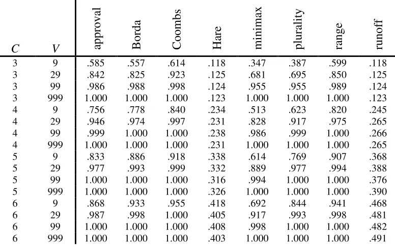
6.2.1. Compromising and burying together: Tables 5-7 and figures 4-6 show the fraction of cases
in which groups strategic voters can elect a mutually preferred candidate by simultaneously burying
the sincere winner and compromising in favor of their preferred candidate. Table 8 compares the
frequency of strategic opportunities using this simple strategy to the overall frequency of strategic
opportunity as determined in the general voting strategy analysis. The last column of the table
shows that taking all of the voting rules together, approximately 94% of the strategically vulnerable
cases in the spatial model, 94% of the vulnerable cases in the impartial model, and 97% of the
vulnerable ANES elections are also vulnerable to this simple strategy. This tells us that the simple
combination of compromising and burying tends to be quite effective, and it tells us that most
examples of strategic vulnerability do not require voters to orchestrate very complex manipulation
schemes to be successful. Thus, looking at figures 4-6, we see that they very closely resemble
Table 5: Analysis V2, compromising and burying, spatial model
V S C approv
al B or da C oombs Ha re mi nim ax plura li ty ra nge runof f
99 1 3 .549 .395 .186 .140 .153 .282 .594 .140
99 2 3 .496 .422 .333 .047 .187 .229 .503 .047
99 4 3 .471 .435 .397 .020 .198 .212 .469 .020
99 8 3 .447 .422 .420 .011 .202 .207 .442 .011
99 16 3 .442 .421 .429 .007 .192 .193 .438 .007
99 1 4 .811 .595 .388 .328 .296 .553 .871 .296
99 2 4 .717 .659 .601 .114 .331 .482 .773 .129
99 4 4 .664 .672 .655 .039 .322 .425 .715 .050
99 8 4 .648 .661 .671 .021 .300 .391 .681 .024
99 16 4 .623 .647 .667 .015 .284 .362 .656 .018
99 1 5 .901 .722 .549 .485 .379 .727 .956 .405
99 2 5 .829 .797 .753 .198 .422 .680 .904 .231
99 4 5 .777 .799 .790 .068 .388 .595 .842 .093
99 8 5 .751 .781 .800 .032 .369 .540 .798 .044
99 16 5 .731 .764 .802 .024 .352 .503 .773 .033
99 1 6 .957 .868 .684 .623 .452 .850 .987 .513
99 2 6 .896 .882 .856 .296 .506 .825 .962 .337
99 4 6 .838 .876 .874 .095 .445 .721 .910 .140
99 8 6 .813 .856 .884 .045 .410 .647 .868 .065
99 16 6 .811 .845 .883 .026 .392 .605 .849 .041
99 4 10 .953 .983 .980 .210 .588 .959 .991 .338
99 4 20 .996 1.000 .999 .504 .712 1.000 1.000 .679
99 4 30 1.000 1.000 1.000 .715 .759 1.000 1.000 .822
Table 6: Analysis V2, compromising and burying, impartial culture model
C V approv
al B or da C oombs Ha re mi nim ax plura li ty ra nge runof f
3 9 .585 .557 .614 .118 .347 .387 .599 .118
3 29 .842 .825 .923 .125 .681 .695 .850 .125
3 99 .986 .988 .998 .124 .955 .955 .989 .124
3 999 1.000 1.000 1.000 .123 1.000 1.000 1.000 .123
4 9 .756 .778 .840 .234 .513 .623 .820 .245
4 29 .946 .974 .997 .231 .828 .917 .975 .265
4 99 .999 1.000 1.000 .238 .986 .999 1.000 .266
4 999 1.000 1.000 1.000 .231 1.000 1.000 1.000 .265
5 9 .833 .886 .918 .338 .614 .769 .907 .368
5 29 .977 .993 .999 .332 .889 .977 .994 .388
5 99 1.000 1.000 1.000 .316 .994 1.000 1.000 .376
5 999 1.000 1.000 1.000 .326 1.000 1.000 1.000 .390
6 9 .868 .933 .955 .418 .692 .844 .941 .468
6 29 .987 .998 1.000 .405 .917 .993 .998 .481
6 99 1.000 1.000 1.000 .408 .998 1.000 1.000 .482
[image:19.612.113.501.464.707.2]Table 7: Analysis V2, compromising and burying, ANES
C approv
al
B
or
da
C
oombs
Ha
re
mi
nim
ax
plura
li
ty
ra
nge
runof
f
3 .605 .545 .656 .020 .277 .291 .587 .020
4 .787 .766 .901 .044 .406 .506 .806 .043
5 .866 .884 .950 .073 .488 .627 .892 .082
[image:20.612.48.572.194.652.2]6 .878 .916 .982 .138 .550 .704 .928 .139
Table 8: Simple strategic opportunities, as share of all opportunities
approv
al
B
or
da
C
oombs
Ha
re
mi
nim
ax
plura
li
ty
ra
nge
runof
f
tot
al
spatial 99% 92% 97% 64% 92% 100% 100% 52% 94%
IC 99% 99% 99% 77% 98% 100% 100% 63% 94%
ANES 100% 99% 99% 60% 98% 100% 100% 52% 97%
average 100% 97% 98% 67% 96% 100% 100% 55% 95%
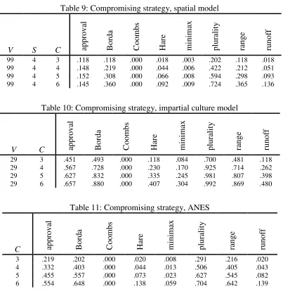
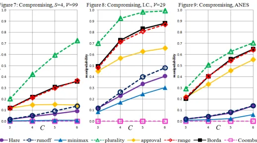
6.2.2. Compromising strategy results: Tables 9-11 and figures 7-9 show the voting rules‘
vulnerability to the compromising strategy, given various specifications. As shown in proposition 4,
compromising strategy, as it is immune to compromising when there is a sincere Condorcet winner.
(This is demonstrated in proposition 5.) Plurality is the most vulnerable to compromising in all
specifications (propositions 7 and 8 show that it is dominated by both Hare and runoff in this
[image:21.612.107.510.164.585.2]respect), and approval, range, and Borda are consistently more vulnerable than Hare and runoff.
Table 9: Compromising strategy, spatial model
V S C approv
al B or da C oombs Ha re mi nim ax plura li ty ra nge runof f
99 4 3 .118 .118 .000 .018 .003 .202 .118 .018
99 4 4 .148 .219 .000 .044 .006 .422 .212 .051
99 4 5 .152 .308 .000 .066 .008 .594 .298 .093
99 4 6 .145 .360 .000 .092 .009 .724 .365 .136
Table 10: Compromising strategy, impartial culture model
V C approv
al B or da C oombs Ha re mi nim ax plura li ty ra nge runof f
29 3 .451 .493 .000 .118 .084 .700 .481 .118
29 4 .567 .728 .000 .230 .170 .925 .714 .262
29 5 .627 .832 .000 .335 .245 .981 .807 .398
29 6 .657 .880 .000 .407 .304 .992 .869 .480
Table 11: Compromising strategy, ANES
C approv
al B or da C oombs Ha re mi nim ax plura li ty ra nge runof f
3 .219 .202 .000 .020 .008 .291 .216 .020
4 .332 .403 .000 .044 .013 .506 .405 .043
5 .455 .557 .000 .073 .023 .627 .545 .082
6.2.3. Burying strategy results: Tables 12-14 and figures 10-12 show the voting rules‘
vulnerability to the burying strategy, given various specifications. As demonstrated in propositions
1-3, plurality, runoff, and Hare are immune to the burying strategy. Coombs, range voting, and
approval voting are consistently the most vulnerable to burying, while Borda and minimax form an
[image:22.612.53.571.65.353.2]intermediate category.
Table 12: Burying strategy, spatial model
V S C approv
al
B
or
da
C
oombs
Ha
re
mi
nim
ax
plura
li
ty
ra
nge
runof
f
99 4 3 .374 .294 .382 .000 .148 .000 .374 .000
99 4 4 .605 .459 .634 .000 .235 .000 .639 .000
99 4 5 .735 .549 .784 .000 .288 .000 .787 .000
Table 13: Burying strategy, impartial culture model
V C approv
al
B
or
da
C
oombs
Ha
re
mi
nim
ax
plura
li
ty
ra
nge
runof
f
29 3 .610 .229 .871 .000 .404 .000 .635 .000
29 4 .786 .267 .986 .000 .407 .000 .865 .000
29 5 .865 .293 .998 .000 .418 .000 .937 .000
29 6 .902 .333 .999 .000 .410 .000 .964 .000
Table 14: Burying strategy, ANES
C approv
al
B
or
da
C
oombs
Ha
re
mi
nim
ax
plura
li
ty
ra
nge
runof
f
3 .495 .297 .647 .000 .209 .000 .448 .000
4 .692 .431 .890 .000 .272 .000 .684 .000
5 .794 .501 .932 .000 .334 .000 .795 .000
6 .827 .538 .979 .000 .328 .000 .873 .000
7. Strategic nomination results
Tables 15-18 and figures 13-16 show the voting rules‘ vulnerability to strategic exit and entry,
frequently vulnerable to strategic exit (proposition 20 gives some intuition for this result), although
with large numbers of candidates in the race, runoff and Hare are vulnerable with similar frequency.
I find that Borda is most vulnerable to strategic entry, and that Coombs is second-most vulnerable.
(Propositions 21 and 22 give some intuition for the vulnerability of Borda and Coombs to strategic
entry.) Minimax is vulnerable to both exit and entry with very low frequency, because its
vulnerability depends on the existence of a majority rule cycle, as demonstrated in propositions 18
[image:24.612.107.508.238.698.2]and 19.
Table 15: Strategic exit, single candidates
S V CO CI Bor
da C oombs Ha re mi nim ax plura li ty runof f
4 99 0 3 .006 .001 .015 .001 .091 .015
4 99 0 5 .013 .002 .060 .004 .251 .093
4 99 0 7 .017 .005 .104 .006 .356 .175
4 99 0 9 .021 .007 .151 .008 .434 .267
4 99 0 11 .018 .011 .193 .010 .490 .344
4 99 0 13 .022 .013 .245 .012 .526 .402
4 99 0 15 .026 .016 .298 .013 .546 .448
4 99 0 19 .027 .021 .389 .015 .588 .532
4 99 0 23 .026 .023 .468 .017 .605 .572
4 99 0 27 .022 .031 .533 .018 .627 .597
4 99 0 31 .027 .035 .587 .018 .641 .624
4 99 0 35 .026 .040 .640 .022 .654 .649
Table 16: Strategic entry, single candidates
S V CI CO Bor
da C oombs Ha re mi nim ax plura li ty runof f
4 99 2 1 .015 .004 .000 .001 .001 .000
4 99 2 2 .029 .006 .000 .001 .004 .000
4 99 2 3 .038 .010 .001 .002 .003 .001
4 99 2 5 .059 .014 .001 .002 .008 .001
4 99 2 7 .065 .018 .002 .002 .009 .002
4 99 2 9 .076 .025 .002 .003 .009 .002
4 99 2 11 .094 .031 .002 .005 .013 .002
4 99 2 13 .103 .036 .002 .005 .016 .002
4 99 2 15 .101 .037 .002 .005 .018 .002
4 99 2 19 .113 .043 .004 .006 .020 .004
4 99 2 23 .118 .050 .004 .008 .020 .004
4 99 2 27 .131 .058 .006 .009 .027 .006
4 99 2 31 .135 .065 .005 .009 .029 .005
Table 17: Candidate groups, strategic exit
V S CI CO Bor
da
C
oombs
Ha
re
mi
nim
ax
plura
li
ty
runof
f
29 4 3 0 .010 .002 .023 .004 .098 .023
29 4 5 0 .033 .009 .084 .011 .331 .119
29 4 7 0 .045 .017 .156 .018 .545 .255
29 4 9 0 .053 .023 .228 .024 .684 .380
29 4 11 0 .063 .030 .305 .031 .790 .506
Table 18: Candidate groups, strategic entry
V S CI CO Bor
da
C
oombs
Ha
re
mi
nim
ax
plura
li
ty
runof
f
29 4 2 1 .042 .013 .002 .004 .010 .003
29 4 2 3 .077 .022 .004 .006 .021 .005
29 4 2 5 .087 .030 .004 .007 .028 .006
29 4 2 7 .108 .038 .007 .011 .035 .009
8. Analytical results
Notation: Let an overscore denote that a variable is defined with respect to voters‘ sincere
preferences; for example, the sincere ranking matrix is , the sincere pairwise matrix is , and so on.
Burying strategy
Proposition 1: Plurality is immune to the burying strategy.
Proof: If voter prefers candidate to the sincere winner , then ‘s sincere ranking will not place
first, which means that will gain zero points from ‘s sincere ballot. If were to attempt to use
a burying strategy against , this would entail giving a worse ranking, , but because both of these rankings give zero points to , the change can‘t affect the outcome of the election. ■
Proposition 2: Runoff is immune to the burying strategy.
Proof: If voter prefers to , then ‘s sincere first-round vote will not be for . Therefore,
can‘t affect whether or not makes it to the second round by burying . If and are both in the second round, then ‘s sincere second-round vote will not be for . Therefore, can‘t help to get
elected by burying . ■
Proof: If voter prefers to , then will be ahead of in ‘s sincere rankings, . may give a still-worse ranking, , but since no ranks behind will be counted unless
is eliminated, this can‘t improve ‘s chances of winning. ■
Note: Minimax, Borda, approval, range, runoff, and Coombs are vulnerable to the burying strategy.
Compromising strategy
Proposition 4: Coombs is immune to the compromising strategy.
Proof: If voter prefers to , then will be ahead of in ‘s sincere rankings, . may give a still-better ranking, , but this can‘t affect the outcome of the race until after
is eliminated. Therefore, the strategy can‘t have an effect until after has been eliminated, and
will not be eliminated until the strategy has an effect. Therefore, the strategy can‘t work. (This is
logically similar to proposition 3 in reverse.) ■
Note: The ‗anti-plurality‘ system, which elects the candidate with the fewest last choice votes, is
another method that is immune to compromising. Plurality, runoff, Hare, minimax, Borda, approval,
and range are all vulnerable to compromising.
Proposition 5: If there is a sincere Condorcet winner, Minimax is not vulnerable to the
compromising strategy.
Proof: If voter prefers to , then will be ahead of in ‘s sincere rankings, which means
that the entry in ‘s sincere individual pairwise matrix will be 1. Formally,
. If voter gives a still-better ranking, this will not change , because
‘s ordering will be unchanged; nor will it change any other , because isn‘t moving in
‘s ranking relative to any other candidate. Formally, , which implies that
.
Because is the sincere Condorcet winner, . Combining this with the above,
, which implies that is still the Condorcet winner and therefore the minimax
winner. ■
Proposition 6: Plurality, runoff, Hare, and minimax are vulnerable to the compromising
strategy when there is a sincere majority rule cycle.
Proof: If there is a sincere majority rule cycle, then for any given sincere winner , there will be
. If all voters rank as their first choice, then will be the winner in plurality,
runoff, Hare, and minimax. ■
Discussion: From propositions 5 and 6, we see that, in the absence of pairwise ties (which are
unlikely in large elections), Plurality, runoff, and Hare are vulnerable to compromising whenever
minimax is vulnerable to compromising, but minimax is not necessarily vulnerable to
compromising when plurality, Hare, or runoff is vulnerable to compromising.
Proposition 7: If plurality isn’t vulnerable to compromising, then runoff isn’t vulnerable to
compromising.
Proof: If plurality isn‘t vulnerable to compromising, then the number of voters whose sincere first
choice is the plurality winner must be greater than the number of voters who prefer any alternative
candidate to . Formally, . Since , must have the most votes, and must advance to the second round of a runoff election, given sincerity. Since
by definition of and , implies that ; that is, must be a Condorcet winner. Therefore, wins the second round (and the election) given sincere voting.
If voters compromise in favor of a candidate , since , will still have the most votes, which means that will still advance into the second round. If advances into the second
round as well, the second round still amounts to a pairwise comparison between and ; because
is a Condorcet winner, will win the runoff. ■
Proposition 8: If plurality isn’t vulnerable to compromising, then Hare isn’t vulnerable to
compromising.
Proof: If plurality isn‘t vulnerable to compromising, then the number of voters whose sincere first
choice is the plurality winner must be greater than the number of voters who prefer any alternative
candidate to . Formally, . Given sincere voting, in any given round of counting, any vote counting for any candidate must come from a voter who prefers to . Therefore, because , and because votes listing as the top choice will be counted for in every round as long as is not eliminated, the number of votes counting for in any given round
must be less than the number of votes counting for . Therefore, can‘t be eliminated in any
round, so will be the sincere winner in Hare.
Given a compromising strategy on behalf of , the logic above will still hold. That is, in any
strategists, and otherwise, the ordering will be reported sincerely. Therefore, will still have the most votes in every round of counting, and will still be the winner in Hare. ■
Discussion: With regard to resistance to the compromising strategy, we see from propositions 7 and
8 that runoff and Hare dominate plurality, and we see from propositions 5 and 6 that all three of
these are all but entirely dominated by minimax.
General voting strategy
Proposition 9: If the sincere Condorcet winner is also the sincere first choice of more than
one third of the voters, then both Hare and runoff will elect and be non-manipulable.
Runoff: Because is the first choice of more than one third of the voters, no group of strategists
will be able to cause his elimination in the first round, because it‘s impossible for two other
candidates to have more than one third of the votes. Because is the Condorcet winner, no
candidate will be able to defeat him in the runoff.
Hare: As in runoff, a candidate with more than first choice votes will not be eliminated before the
last round, because each of the prior rounds will include three or more candidates, and because none
of the voters whose sincere first choice is will have an incentive to defect on behalf of an
alternative candidate . Because the last round is equivalent to a pairwise comparison, and because
is the Condorcet winner, will win. ■
Note: The property described in proposition 9 is not shared by plurality, minimax, Borda, Coombs,
approval, or range.
Proposition 10: Given the Hare system, with candidates , if there are voters with each possible preference ordering, plus one additional voter with an preference ordering (a set of ‘almost symmetrical’ preferences), will be the winner, and the result will
not be manipulable.
Proof: In the first round of counting, , and , . That is, the votes are divided evenly, except for the one extra vote that gives his advantage. Strategists
can‘t cause to be eliminated in the first round, because is the first choice of more than
voters, which means that it‘s not possible for strategists to arrange for all of the other candidates to
Similar logic holds in later rounds of counting. That is, when candidates remain, no candidate
can have the fewest first choice votes if he has at least votes; because will have
sincere votes, he can‘t be eliminated. Because is their first choice among non-eliminated
candidates, none of these voters will be interested in participating in a strategy on behalf of any
non-eliminated candidate . Therefore, strategic incursion against can‘t succeed. ■
Discussion: The purpose of propositions 10 through 12 is to shed some light on a dynamic observed
in the impartial culture simulation results: Given , Hare is the only one of my eight voting
methods that doesn‘t converge towards 100% manipulability as the number of voters gets large.
Given , this property is shared by the runoff system. When is large in an impartial culture model, each preference order appears in approximately equal proportion; therefore, the winner‘s
margin of victory tends to be very small relative to the number of voters who prefer an alternative
candidate to the sincere winner. These features are captured in the ‗almost symmetrical preferences‘ scenario that provides the basis for these propositions.
Proposition 11: Given candidates , if there are voters with each possible preference ordering, plus one additional voter with an preference ordering, the result will be manipulable in plurality, minimax, Borda, and Coombs, given a sufficiently
large value of .
Plurality: With first choice votes (where ), to every other candidate‘s first
choice votes, is the sincere winner. For any , the number of potential strategists is
given by , which is greater than , for
. Therefore, if these strategists
vote for , will win.
Minimax: For , , and for , . Therefore, for ,
, and for all other , . Therefore, is the sincere winner.
Suppose, however, that all of the voters who prefer vote .
Then, we still have , but now, , and
Borda: From the sincere pairwise matrix described above, we calculate that the sincere Borda
score for each candidate is , and the sincere winner is .
Suppose, however, that all of the voters who prefer vote . The
resulting pairwise matrix will be
, and the
resulting Borda scores will be , , and
, . Therefore, the new winner will be .
Coombs: Given sincere voting, each candidate will have the same number of last choice votes in
each round of counting, except for the one symmetry-breaking vote, which will cause the
elimination order to be , so that is the winner. However, if the voters who prefer
change their votes so that is ranked last, but the rankings are otherwise the same, will
be eliminated in the first round (with last choice votes, which is greater than ‘s total of
last choice votes), and then the remaining eliminations will occur in their original order,
leaving as the winner. ■
Proposition 12: Given the runoff system, with candidates , if there are voters with each possible preference ordering, plus one additional voter with an preference ordering, will be the winner. If , the result will not be manipulable, but if , the result will be manipulable.
Case 1, : Because is the sincere Condorcet winner, and because has more than votes,
is the sincere winner, and the result is non-manipulable, by proposition 9 above.
Case 2, : As in the case, is the sincere winner. has first choice votes,
and there are voters who prefer . Aside from these voters, has
first
choice votes. The voters can prevent from reaching the runoff by distributing their votes
between and so that has fewer votes than each of them. This requires