Selection of Control Variables in Propensity Score Matching: Evidence from a Simulation Study

Munich Personal RePEc Archive

Selection of Control Variables in

Propensity Score Matching: Evidence

from a Simulation Study

Nguyen Viet, Cuong

10 February 2012

1

Selection of Control Variables in Propensity Score Matching:

Evidence from a Simulation Study

Nguyen Viet Cuong1

Institute of Public Policy and Management National Economics University

Abstract

Propensity score matching is a widely-used method to measure the effect of a treatment in

social as well as health sciences. An important issue in propensity score matching is how to

select conditioning variables in estimation of the propensity score. It is commonly

mentioned that only variables which affect both program participation and outcomes are

selected. Using Monte Carlo simulation, this paper shows that efficiency in estimation of

the Average Treatment Effect on the Treated can be gained if all the available observed

variables in the outcome equation are included in the estimation of the propensity score.

Keywords: Impact evaluation, treatment effect, propensity score matching, covariate

selection, Monte Carlo.

JEL classification codes: H43, C15, C14.

1

Institute of Public Policy and Management, National Economics University, Hanoi, Vietnam.

2

1. Introduction

Matching is a popular method to measure the effect of a treatment on a group of subjects.

There is a large amount of literature on matching methods of impact evaluation (see

Heckman et al., 1997; Augurzky and Schmidt, 2001; Imbens and Wooldridge, 2009). The

basic idea of the matching method is to find a control group (also called comparison group)

that has a similar distribution of control variables as the treatment group. By the same

token, the difference in the control variables between the treatment and control groups is

controlled for. Under the conditional independence assumption, the difference in outcomes

between the control group and the treatment group then can be attributed to the program

impact. The matching method can be combined with difference-in-differences (e.g., see

Smith and Todd, 2005) as well as with instrumental variables (Ichimura and Taber, 2001)

to relax the conditional independence assumption. Compared with parametric estimation,

the matching method has the main advantage that it does not impose a functional form

assumption on outcome.

Since a paper by Rosenbaum and Rubin (1983), matching is often performed based

on the probability of being assigned to the program given observed conditioning variables,

which is called the propensity score. A control group is matched with a treatment group

based on closeness of the propensity score. Propensity score matching is a widely applied

in social as well as health sciences (e.g., Heckman et al., 1997; Imbens and Wooldridge,

2009).

Since the propensity score is often unobserved, we have to estimate it using a

regression of program participation on conditioning variables. An important issue in the

3

Most studies argue that only variables which affect both the program participation and

outcomes should be included in the estimation of the propensity score (e.g., Heckman et al.,

1998; Ravallion, 2001; Augurzky and Schmidt, 2001; Bryson et al., 2002; Lechner, 2002;

Caliendo and Kopeinig, 2008). Bryson et al. (2002) mentioned that inclusion of irrelevant

variables can increase variances of estimates. Recently, Zhao (2008) found that

over-specification of the model of the propensity score can bias impact estimates. However,

none of these studies present a detailed discussion on why only variables which affect both

the treatment and outcomes should be controlled in the propensity score estimation.

In OLS, adding more control relevant variables can increase efficiency of the

model, and the standard error of a variable of interest can be reduced. However, inclusion

of more variables can result in multicollinearity, which can increase the standard error of

the variable of interest. Matching can avoid the multicollinearity problem, and a question

on whether inclusion of variables affecting outcome but not program participation in the

estimation of the propensity score can increase the efficiency of impact estimates remains

unanswered. This paper uses Monte Carlo simulations to examine whether we should

control for all the available observed variables in the outcome equation or only variables

which simultaneously affect outcome and program participation. The Monte Carlo

simulations are used to assess the efficiency of the propensity score matching estimator,

since there have been no asymptotic properties derived for propensity score estimators in

the case of unknown propensity score (Imbens and Wooldridge, 2009). To examine the

properties of matching estimators, many studies rely on Monte Carlo simulations (e.g.,

Frölich, 2004; Zhao, 2004; Austin, 2007; Zhao, 2008, Ghosh, 2011).

The paper is structured as follows. The second section reviews the propensity score

4

The third section presents Monte Carlo simulations. Finally, the fourth section presents

conclusions.

2. Propensity score matching

2.1. Matching method

Denote by D the binary variable of participation in a program, i.e. D=1 for participants,

and D=0 for non-participants. Let Y₁ and Y₀ denote the potential outcomes in states of

program and no-program, respectively.2 The most popular parameter in impact evaluation is the Average Treatment Effect on the Treated (ATT) (Heckman et al., 1999):

) 1 (

) 1

( ₁ = − ₀ =

=E Y D E Y D

ATT . (1)

ATT is the impact of the program on the participants. Estimation of ATT is not

straightforward, since the counterfactual term E(Y0|D=1) is not observed. E(Y0 |D=1) is

the expected outcome of the participants had they not participated in the program. The

matching method identifies ATT based on a conditional independence assumption (CIA): 3

X D Y

Y0, 1⊥ . (2)

Under CIA, ATT are identified. First, ATT conditional on X is identified:

) 0 , | ( ) 1 , | ( ) 1 , | ( ) 1 , |

( _{1 0 1 0}

)

( =E Y X D= −E Y X D= =E Y X D= −E Y X D=

ATTX (3)

Then ATT is also identified, since:

2

In literature of impact evaluation, a broader term “treatment” instead of program/project is sometimes used to refer an intervention whose impact is evaluated. In this paper, an intervention, a treatment and a program are used interchangeably.

3

We just need a weaker assumption (so-called the conditional mean independence assumption) to identify the program. The assumptions are:

) | ( ) , |

(Y0 X D E Y0 X

E = ,

) | ( ) , |

(Y1 X D E Y1 X

5

= =

=

1

|D ( )dF(X| 1) X ATTX D

ATT (4)

For the matching method to be implemented, we must find a control group that is similar to

the treatment group but does not participate in the program. This similarity assumption is

called common support. If we denote p(X) as the probability of participating in the program for each subject, i.e. p(X)=P(D=1|X), the assumption can be stated formally as

1 ) (

0< p X < . The difference in outcome of the control group and the treatment group then

can be attributed to the program impact.

2.2. Propensity score matching

As mentioned, the comparison group is constructed by matching each participant in the

treatment group with one or more non-participants whose variables X are closest to X of

the participants. The weighted average outcome of non-participants who are matched with

an individual participant will form the counterfactual outcome for the participant.

Matched non-participants should have X closest to X of participants. X is often a vector of variables, and finding “close” non-participants to match with a participant is not

straightforward. A widely-used way to find the matched sample is the propensity score

matching. Since a paper by Rosenbaum and Rubin (1983), matching is often conducted

based on the probability of being assigned to the program, which is called the propensity

score. Rosenbaum and Rubin (1983) show that if the potential outcomes are independent of

6

popular balancing score is the propensity score. The propensity score can be estimated by

running a probit or logit regression of D on the X variables.

Each participant is matched with one or several non-participants. One can select

different methods to weight outcomes of these matched non-participants. If each participant

is matched with one non-participant, the weight equals one for all pairs of matches. This is

called one nearest neighbor matching. When more than one non-participant are matched

with each participant (or vice versa), we need some ways to define the weights attached to

each non-participant.

A number of methods use equal weights for all matches. N-nearest neighbor

matching involves matching each participant with n non-participants, and each matched non-participant will receive equal weights 1/n. However, it could be reasonable to assign

different weights to different non-participants depending on metric distances between their

covariates and the covariates of the matched participant. This argument motivates some

others matching schemes such as kernel, local linear matching (see, e.g., Heckman et al.,

1997; Smith and Todd, 2005), and matching using weights of inversed propensity score

(see, e.g., Hahn, 1998; Hirano et al., 2003).

3. Monte Carlo simulations

An important practical issue in the application of the propensity score matching is selection

of control variables in estimating the propensity score. Most studies claim that only

variables which affect both the program participation and outcomes should be included in

7 Augurzky and Schmidt, 2001; Bryson et al., 2002; Lechner, 2002; Caliendo and Kopeinig,

2008). Yet, none of these studies present a detailed discussion on why only variables

affecting both the treatment and outcomes should be controlled. This section examines

whether we should control for all the available observed variables in the outcome equation

or only variables which simultaneously affect outcome and program participation in the

propensity score matching using simulations of estimation of ATT of a program D.

The simulation study is designed as follows. First, the program participation is

designed as follows:

u z x

x

d =0.5 1+0.5 2+0.5 + , (5)

1

=

D if d>d*, D=0 otherwise. d*is set equal to the 75th percentile of dso that a quarter of observations have D equal to 1. Variables x and z follow normal distributions

) 5 , 10 ( ) ,

( N

N µ σ = , and error term u follows a normal distribution N(µ,σ)= N(0 ,5).

Second, potential outcomes are functions of covariates x and error terms as

follows:

y0=10+β0_1x1+β0_2x2+β0_3x3+β0_4x4+β0_5x5+β0_6x6 +ε0, (6)

y1 =10+β1_1x1+β1_2x2 +β1_3x3+β1_4x4+β1_5x5+β1_6x6+ε1, (7)

where each x follows a normal distribution N(µ,σ)=N(10 ,5), and each error term follows

a normal distribution N(µ,σ)=N(0,5). The impact of program D are changed by varying

the value of β. x1 and x2 affect both outcomes and the program participation. Variables

from x₃ to x₆ affect outcomes but not the program participation. Variable z affects the

program participation but not the outcome (z is can be regarded as an instrumental variable

8 We present results from two matching estimators including three-nearest-neighbors

matching and kernel matching with bandwidth of 0.01.4 Results from other matching estimators including one-nearest-neighbors, five-nearest-neighbors, kernel matching with

other bandwidths (0.005 and 0.05), local linear regression matching with different

bandwidths (0.005, 0.01 and 0.05) are similar and have the same trend as the

three-nearest-neighbors matching and kernel matching with bandwidth of 0.01. These results are not

presented in this paper.5 The propensity score is estimated using a probit model, i.e.

(

)

(

)

P = =Φ + where X is a vector of the x variables. We consider different

sample sizes of observations: n equals 200, 500 and 1000. The number of replications is

1000.

We examine the sensitivity of the propensity score matching estimates to selection

of conditioning variables in different simulation scenarios as follows.

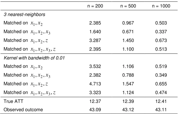
Scenario 1:The outcome equations include x₁,x₂ and x₃ as follows:

y0 =10+x1+x2 +x3+ε0, (8)

1 3 2 1

1=10+1.5x +1.5x +x +ε

y . (9)

The impact of D is through increased coefficients of x₁ and x₂. Table 1 presents the

results under scenario 1. The table reports the mean-squared error (MSE) for different sets

of covariates used in the propensity score matching. It shows that the propensity score

matching has lower MSE when all the three x variables including x3 - which affects the

outcome but not the program participation - are included in the estimation of the propensity

score. However, inclusion of z increases MSE.

4

The standard error for the nearest-neighbor matching estimator using bootstrapping might not be valid (Abadie and Imbens, 2008). However, there are no evidences against the standard error of other propensity score matching estimators computed using bootstrap. In addition, in this study we assess the mean-squared error of the propensity score matching estimators.

5

9 Table 1. MSE in scenario 1

n = 200 n = 500 n = 1000

3 nearest-neighbors

Matched on _x1,x2 2.385 0.967 0.503

Matched on

3 2 1,x ,x

x 1.640 0.671 0.337

Matched on _x1,x2,z 3.287 1.450 0.673

Matched on _{x,x ,x ,z} 3 2

1 2.395 1.100 0.513

Kernel with bandwidth of 0.01

Matched on _x1,x2 3.532 1.106 0.519

Matched on

3 2 1,x ,x

x 2.382 0.788 0.349

Matched on _x1,x2,z 4.713 1.547 0.655

Matched on _{x,x ,x ,z} 3 2

1 3.323 1.124 0.474

True ATT 12.37 12.39 12.41

Observed outcome 43.09 43.12 43.11

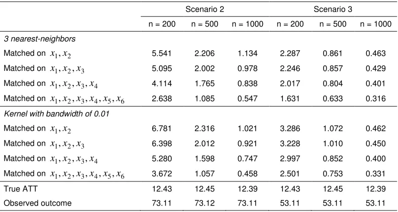
Scenario 2: The outcome equations include all the variables fromx₁ to x₆ as follows:

0 6 5 4 3 2 1

0 =10+x +x +x +x +x +x +ε

y , (10)

y1=10+1.5x1+1.5x2 +x3+x4+x5+x6+ε1, (11)

Scenario 3:The role of variables x3 to x6 is lower than that in scenario 2. The outcome

equations are as follows:

y0=10+x1+x2+0.5x3+0.5x4+0.5x5+0.5x6+ε0, (12)

1 6 5 4 3 2 1

1=10+1.5x +1.5x +0.5x +0.5x +0.5x +0.5x +ε

y , (13)

Table 2 shows that the propensity score matching yields lower MSE as the number of

covariates used in the propensity score estimation increases. The value of MSE is much

smaller when all variables which affect outcome are controlled in the estimation of the

10 Table 2. MSE in scenarios 2 and 3

Scenario 2 Scenario 3

n = 200 n = 500 n = 1000 n = 200 n = 500 n = 1000

3 nearest-neighbors

Matched on _x1,x2 5.541 2.206 1.134 2.287 0.861 0.463

Matched on

3 2 1,x ,x

x 5.095 2.002 0.978 2.246 0.857 0.429

Matched on _x1,x2,x3,x4 4.114 1.765 0.838 2.017 0.804 0.401 Matched on 6 5 4 3 2

1,x ,x ,x ,x ,x

x 2.638 1.085 0.547 1.631 0.633 0.316

Kernel with bandwidth of 0.01

Matched on _x1,x2 6.781 2.316 1.021 3.286 1.072 0.462

Matched on

3 2 1,x ,x

x 6.398 2.012 0.921 3.228 1.010 0.450

Matched on _x1,x2,x3,x4 5.280 1.598 0.747 2.997 0.852 0.400 Matched on 6 5 4 3 2

1,x ,x ,x ,x ,x

x 3.672 1.057 0.458 2.501 0.753 0.331

True ATT 12.43 12.45 12.39 12.43 12.45 12.39

Observed outcome 73.11 73.12 73.11 53.11 53.11 53.11

Scenario 4:This scenario has similar outcome equations as scenario 3, but the x variables

are allowed to be correlated with a pairwise correlation coefficient of 0.5.

Scenario 5: The outcome equations are quadratic functions of the x variables as follows:

0 2 6 2 5 2 4 2 3 2 2 2 1

0=10+0.1x +0.1x +0.1x +0.1x +0.1x +0.1x +ε

y , (14)

1 2 6 2 5 2 4 2 3 2 2 2 1

1=10+0.15x +0.15x +0.1x +0.1x +0.1x +0.1x +ε

y . (15)

Tables 3 shows that for both scenarios 4 and 5, the propensity score matching still has the

lowest MSE when controlling for all the x variables.

Table 3. MSE in scenarios 4 and 5

Scenario 4 Scenario 5

n = 200 n = 500 n = 1000 n = 200 n = 500 n = 1000 3 nearest-neighbors

Matched on _x1,x2 3.980 1.279 0.642 22.712 9.546 4.434

Matched on

3 2 1,x ,x

x 3.693 1.225 0.618 21.322 8.330 3.798

Matched on _x1,x2,x3,x4 3.571 1.180 0.554 17.775 7.348 3.214 Matched on 6 5 4 3 2

1,x ,x ,x ,x ,x

x 3.584 1.035 0.501 11.210 4.422 2.143

Kernel with bandwidth of 0.01

Matched on _x1,x2 4.522 1.579 0.673 30.061 10.848 4.297

Matched on

3 2 1,x ,x

x 4.066 1.448 0.616 29.470 9.197 3.906

11

Scenario 4 Scenario 5

n = 200 n = 500 n = 1000 n = 200 n = 500 n = 1000 Matched on 6 5 4 3 2

1,x ,x ,x ,x ,x

x 4.343 1.281 0.506 17.852 5.366 2.200

True ATT 13.33 13.42 13.37 17.66 17.68 17.59

Observed outcome 53.32 53.35 53.37 89.45 89.47 89.42

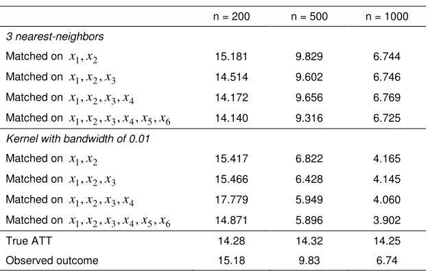
Scenario 6: This scenario has similar outcome equations as scenario 3. However, the

selection equation is set up as follows:

u z x x

d =3 1+3 2+ + (16)

It means that D depends strongly on x1 and x2. Pseudo-R2 of the probit regression on x1

and x2is very high, at 0.7. Similarly to previous scenarios, the propensity score matching

which controls for all the variables in the outcome equations has the smallest MSE.

However, the differences in MSE between the case of controlling for all the variables and

the case of controlling for x₁ and x₂are very small. MSE is very high, since the common

support is small.

Table 4. MSE in scenario 6

n = 200 n = 500 n = 1000

3 nearest-neighbors

Matched on x_1,x₂ 15.181 9.829 6.744

Matched on

3 2 1,x ,x

x 14.514 9.602 6.746

Matched on x_1,x_2,x_3,x₄ 14.172 9.656 6.769

Matched on 6 5 4 3 2

1,x ,x ,x ,x ,x

x 14.140 9.316 6.725

Kernel with bandwidth of 0.01

Matched on x_1,x₂ 15.417 6.822 4.165

Matched on

3 2 1,x ,x

x 15.466 6.428 4.145

Matched on x_1,x_2,x_3,x₄ 17.779 5.949 4.060

Matched on 6 5 4 3 2

1,x ,x ,x ,x ,x

x 14.871 5.896 3.902

True ATT 14.28 14.32 14.25

12

4. Conclusions

Propensity score matching is a widely-used method to measure the effect of a treatment on

the treated. An important issue in the propensity score matching is how to select control

variables in estimating the propensity score. It is commonly argued that only variables

which simultaneously affect outcomes and program participation should be included as

covariates in the propensity score matching. Yet, using Monte Carlo simulations this paper

shows that the efficiency in estimation of the ATT can be gained if all the variables in the

outcome equation including those not affecting the program participation are used in the

propensity score matching. However, variables which affect the program participation but

not outcomes should not be used in the propensity score matching. Using these variables in

estimation of the propensity score tends to increase the MSE of the propensity score

matching estimator.

Finally, it should be noted that Monte Carlo only provides analytical evidences in

specific cases. A general treatment of properties of the propensity score matching

13

References

Abadie, A., and Imbens G. W. (2008), “On the Failure of the Bootstrap for Matching

Estimators”, Econometrica, Vol. 76(6), 1537-1557.

Augurzky, B. and Schmidt, C.M. (2001), “The Propensity Score: a Means to an End”, IZA

Discussion Paper Series No. 271.

Austin, P. C. (2007), “The Performance of Different Propensity Score Methods For

Estimating Marginal Odds Ratios”, Statistics in Medicine, 26, 3078–3094.

Bryson, A., R. Dorsett, and S. Purdon (2002), “The Use of Propensity Score Matching in

the Evaluation of Labour Market Policies," Working Paper No. 4, Department for Work

and Pensions.

Caliendo, M. and S. Kopeinig (2008), “Some Practical Guidance for the Implementation of

Propensity Score Matching”,Journal of Economic Surveys, 22(1), 31–72.

Feng, P., Zhou, X.-H., Zou, Q.-M., Fan, M.-Y. and Li, X.-S. (2011), “Generalized

Propensity Score for Estimating the Average Treatment Effect of Multiple Treatments”,

Statistics in Medicine, 30: n/a. doi: 10.1002/sim.4168

Frölich, M. (2004), “Finite Sample Properties of Propensity-Score Matching and Weighting

Estimators”, Review of Economics and Statistics, 86(1), 77-90.

Ghosh D. (2011), “Propensity Score Modeling in Observational Studies using Dimension

Reduction Methods”, Statistics & Probability Letters, 81(7), 813-820.

Hahn, J. (1998), “On the Role of the Propensity Score in Efficient Semiparametric

14 Heckman, J., H. Ichimura, and P. Todd (1997), “Matching as an Econometric Evaluation

Estimators: Evidence from Evaluating a Job Training Programme”, Review of Economic

Studies, 64(4), 605- 654.

Heckman, J., R. Lalonde and J. Smith (1999). The Economics and Econometrics of Active

Labor Market Programs. Handbook of Labor Economics, Volume 3, Ashenfelter, A. and D.

Card, eds., Amsterdam: Elsevier Science.

Heckman, J; Ichimura, H; Smith, J; and Todd, P. (1998), “Characterizing Selection Bias

using Experimental Data”, Econometrica, 66, 1017-1098.

Hirano K., G. W. Imbens and G. Ridder (2002), “Efficient Estimation of Average

Treatment Effects using the Estimated Propensity Score”, Econometrica, 71(4), 1161-1190.

Ichimura, Hidehiko and Taber Christopher (2001), “Propensity-Score Matching with

Instrumental Variables”, American Economic Review, 91(2): 119-124.

Imbens, G., and Wooldridge, J. (2009), “Recent Developments in the Econometrics of

Program Evaluation”, Journal of Economic Literature, Vol 47(1), 5-86.

Lechner, M. (2002), “Some Practical Issues in The Evaluation of Heterogeneous Labour

Market Programmes by Matching Methods”, Journal of the Royal Statistical Society. Series

A, 165, 59-82.

Ravallion, M. (2001), “The Mystery of the Vanishing Benefits: An Introduction to Impact

Evaluation”, The World Bank Economic Review, 15(1), 115-140.

Rosenbaum, P. and R. Rubin (1983), “The Central Role of the Propensity Score in

Observational Studies for Causal Effects”, Biometrika 70 (1), 41-55.

Rosenbaum, P. and R. Rubin (1985), “Constructing a Control Group Using Multivariate

Matched Sampling Methods that Incorporate the Propensity Score”, American Statistician,

15 Smith, J. and P. Todd. (2005), “Does Matching Overcome LaLonde’s Critique of

Nonexperimental Estimators?”, Journal of Econometrics, 125(1–2), 305–353.

Zhao, Z. (2004), "Using Matching to Estimate Treatment Effects: Data Requirements,

Matching Metrics, and Monte Carlo Evidence," The Review of Economics and Statistics,

86(1), 91-107.

Zhao, Z. (2008), “Sensitivity of propensity score methods to the specifications”, Economics