Discharge estimation in a backwater affected meandering river

Utrecht, The Netherlands

Received: 4 March 2011 – Published in Hydrol. Earth Syst. Sci. Discuss.: 9 March 2011 Revised: 10 August 2011 – Accepted: 22 August 2011 – Published: 30 August 2011

Abstract. Variable effects of backwaters complicate the

de-velopment of rating curves at hydrometric measurement sta-tions. In areas influenced by backwater, single-parameter rat-ing curve techniques are often inapplicable. To overcome this, several authors have advocated the use of an additional downstream level gauge to estimate the longitudinal surface level gradient, but this is cumbersome in a lowland mean-dering river with considerable transverse surface level gra-dients. Recent developments allow river flow to be con-tinuously monitored through velocity measurements with an acoustic Doppler current profiler (H-ADCP), deployed hor-izontally at a river bank. This approach was adopted to ob-tain continuous discharge estimates at a cross-section in the River Mahakam at a station located about 300 km upstream of the river mouth in the Mahakam delta. The discharge station represents an area influenced by variable backwater effects from lakes, tributaries and floodplain ponds, and by tides. We applied both the standard index velocity method and a recently developed methodology to obtain a continu-ous time-series of discharge from the H-ADCP data. Mea-surements with a boat-mounted ADCP were used for cali-bration and validation of the model to translate H-ADCP ve-locity to discharge. As a comparison with conventional dis-charge estimation techniques, a stage-disdis-charge relation us-ing Jones formula was developed. The discharge rate at the station exceeded 3250 m3s−1. Discharge series from a tra-ditional stage-discharge relation did not capture the overall discharge dynamics, as inferred from H-ADCP data. For a specific river stage, the discharge range could be as high as 2000 m3s−1_{, which is far beyond what could be explained} from kinematic wave dynamics. Backwater effects from lakes were shown to be significant, whereas interaction of the river flow with tides may impact discharge variation in

Correspondence to: H. Hidayat (hidayat.hidayat@wur.nl)

the fortnightly frequency band. Fortnightly tides cannot eas-ily be isolated from river discharge variation, which features similar periodicities.

1 Introduction

Discharge is the phase in the hydrological cycle in which water is confined in channels, allowing for an accurate mea-surement compared to other hydrological phases (Herschy, 2009). Reliable discharge data is vital in research focus-ing on a broad range of topics related to water manage-ment, including water allocation, navigation, and the predic-tion of floods and droughts. Also, it is crucial in catchment-scale water balance evaluations. Hydrological studies rely-ing on rainfall-runoff models require continuous discharge series for model calibration and validation (e.g. Beven, 2001; McMillan et al., 2010).

Single-valued rating curves can produce biased discharge estimates, especially in highly dynamic rivers and streams. In terms of the momentum equation, this bias is the result of temporal and spatial acceleration terms, and the pressure gra-dient term, which all have to be neglected to justify an unam-biguous relation between stage and discharge. River waves featuring such unambiguous relation are termed kinematic. When the pressure gradient term is retained, but the acceler-ation terms can be neglected, the momentum balance appears as a convection-diffusion equation that can be solved to yield a non-inertial wave as a special type of diffusion wave (Yen and Tsai, 2001). Several formulas have been developed aim-ing to obtain discharge from parameters that can readily be derived from water level time-series. Among these, the Jones formula (Jones, 1916) is the most well-known, in which the surface level gradient term is approximated using the kine-matic wave equation. The Jones’ formula has been subject to many investigations since its publication (see Schmidt, 2002 and Dottori et al., 2009 for a review). Strictly speaking, it may be more correct to refer to the formula as the Jones-Thomas formula, as it was Jones-Thomas who replaced the spa-tial derivative term by a temporal derivative term, in order to enable estimating the discharge from at-a-station stage mea-surements (A. D. Koussis, personal communication, 2011).

Variable backwater is one of the principle factors that cause an ambiguous stage-discharge relation. Backwater from one or several downstream elements such as tributaries, lakes, ponds or dams, complicates rating curve development at hydrometric gauging stations (Petersen-Overleir and Rei-tan, 2009). Tides superimposed on river discharge can pro-duce subtidal water level variations (Buschman et al., 2009), with periods of a fortnight or longer, which may not imme-diately be recognized as phenomena controlled by the tidal motion. Potentially, water level setup by river-tide interac-tions can cause backwater effects beyond the point of tidal extinction (Godin and Mart´ınez, 1994).

Recently, approaches have been developed to account for backwater effects, using a twin gauge approach to obtain es-timates of the longitudinal water level gradient. Such ratings are developed based on records of stage at a base gauge and the fall of the water surface between the base gauge and a second gauge downstream (Herschy, 2009). Considering the water level gradient to be a known variable, the terms repre-senting the pressure gradient and spatial acceleration in the momentum equation can be resolved (Dottori et al., 2009). The application of formulas using simultaneous stage mea-surements was criticised by Koussis (2010). Dottori and To-dini (2010) refuted most of the criticism by Koussis (2010), but acknowledged that in lowland areas with a small bed level gradient, the occurring water level gradient can drop be-low the measuring accuracy of the level gauge. Dottori and Todini (2010) estimate the minimum distance between the gauges to be in between 2000 and 5000 m when the bed slope is 1×10−5. Since cross-profiles of the water level are not taken into consideration in one dimensional river hydraulics,

neither Koussis (2010) nor Dottori and Todini (2010) consid-ered the drawback that arises from lateral water level gra-dients, which can be considerable especially in meandering rivers characterised by a high sinuosity. In high-curvature river reaches, level gauges on opposite sides of each of the two cross-section would be needed to infer the longitudinal water surface gradient. We conclude that the twin gauge ap-proach to discharge measurements is suboptimal in lowland meandering rivers, which are most susceptible to backwater effects.

Discharge can be estimated from flow velocity, which bears a much stronger relation to discharge than the water surface. Gordon (1989) was among the first to estimate dis-charge from a boat-mounted acoustic Doppler current pro-filer (ADCP), which soon after became a standard means of estimating discharge accurately. ADCP surveys are costly and are carried out merely occasionally. Recent develop-ments allow horizontal profiles of flow velocity to be contin-uously monitored by a horizontal acoustic Doppler current profiler (H-ADCP). The H-ADCP is typically deployed at a river bank, measuring a horizontal velocity profile across a channel. The acquired data can then be used to estimate dis-charge, predicting cross-section integrated velocity from the array data of flow velocity.

Several methods are available to convert H-ADCP data to discharge. In the Index Velocity Method (IVM), H-ADCP velocity estimates are averaged and linearly regressed with those obtained from boat-mounted ADCP measurements, then discharge is obtained from the area-velocity relation (Simpson and Bland, 2000; Le Coz et al., 2008). Nihei and Kimizu (2008) adopted a deterministic approach, as-similating H-ADCP data with a two-dimensional model of the velocity distribution over a river cross-section. In the velocity profile method (VPM) described by Le Coz et al. (2008), total discharge is inferred from theoretical vertical velocity profiles, made dimensional with the H-ADCP ve-locity measurements across the section, extrapolated over the river width. Hoitink et al. (2009) combined elements of the IVM and VPM methods, using a boundary layer model to calculate specific discharge from a point measurement of ve-locity, and a regression model to relate specific discharge to total discharge. Sassi et al. (2011) elaborated on the work of Hoitink et al. (2009) by embedding a more sophisticated boundary layer model that accounts for side wall effects in the methodology, and letting model coefficients be stage de-pendent instead of constant. Whereas both Hoitink et al. (2009) and Sassi et al. (2011) focused on tidal rivers, the present contribution presents an H-ADCP deployment in a backwater affected inland river.

Fig. 1. Location of H-ADCP discharge station in the Mahakam River, plotted on a digital elevation model obtained from Shuttle Radar

Topographic Mission (SRTM) data.

presents the results and a discussion and in Sect. 5 conclu-sions are drawn.

2 Study area and data gathering

This study is based on measurements carried out in the River Mahakam, which drains an area of about 77 100 km2 in East Kalimantan, Indonesia. The H-ADCP measurement station is located in Melak in the middle Mahakam area about 300 km from the delta apex (Fig. 1). The middle Ma-hakam area is an extremely flat tropical lowland with some thirty shallow lakes connected to the Mahakam through small channels. It can be considered a remote, poorly gauged re-gion. A tributary, River Kedang Pahu, meets the Mahakam about 30 km downstream of Melak. Downstream of the lakes region, the Mahakam is tied to three other main trib-utaries (River Belayan, Kedang Kepala, and Kedang Rantau) and flows south-eastwards until the discharge is divided over delta distributaries debouching into the Makassar Strait.

The H-ADCP discharge measurement station was opera-tional at a 270 m wide cross section of the Mahakam river in Melak (Fig. 2) between March 2008 and August 2009. A 600 kHz H-ADCP manufactured by RD Instruments was mounted on a solid jetty in the concave side of the river bend. Riverbanks at this particular location are quite steep, leading to a cross-section with a relatively confined flow, except at very high and unusual discharges. The H-ADCP was mounted at about 2.5 m below the lowest recorded water level and about 2 m from the bottom. Pitch and roll of the instrument remained relatively constant during the measur-ing period, amountmeasur-ing to 0.3◦ and 0.01◦, respectively. The measurement protocol for the H-ADCP consisted in 10 min bursts at 1 Hz every 30 min.

Fig. 2. Top: bathymetry at Melak discharge gauging station. The

arrow indicates flow direction, V indicates the location where the H-ADCP was deployed, double arrows indicate locations of boat-mounted ADCP transects. Bottom: channel cross-sectional profile at the station. The shaded area indicates cross-section of the H-ADCP conical measuring volume,dis the distance of the H-ADCP below the mean water level,His mean water depth,ηis water level variation, andzis normal distance from the bed.

level was used as the reference water level. Because the H-ADCP was deployed looking slightly upward, the H-H-ADCP measured a volume-averaged velocity at elevationzc, which is calculated from:

zc=

(

−d+tan(θ )(n−x) if d+η >tan(φ/2+θ )(n−x) −d+tan(θ )(n−x)+1z otherwise

(1) whereθis pitch,nis cross-channel coordinate, with the ori-gin at the river bank andηis water level variation.1zis the level difference between the centroid of the ensonified water area and the central beam axis. This correction accounts for the lowering of the centroid of the ensonified water volume if the main lobe intersects with the water surface at low water (Hoitink et al., 2009).

Conventional boat-mounted ADCP measurements were periodically taken at the cross-section where the H-ADCP was deployed to establish water discharge through the river section. Six surveys were carried out spanning low and high flow conditions. The survey consisted of transects in front of the H-ADCP for determining hydraulic parameters (referred to as “par”) and transects carried out about 20 m upstream to cover the whole river section for calibrating and validating the discharge computation (referred to as “cal” and “val”, re-spectively). Each transect measurement spanned over about two hours. The boat was equipped with a 1.2 MHz RDI Broadband ADCP measuring in mode 12, a DGPS compass and an echosounder. The ADCP measured a single ping ensemble at approximately 1 Hz with a depth cell size of 0.35 m. Each ping was composed of 6 sub-pings, separated by 0.04 s. The range to the first cell center was 0.865 m. The boat speed ranged between 1 and 3 m s−1_.

Recently, Moore et al. (2010) found that H-ADCP data can be flawed by the effect of acoustic side lobe reflections from the water surface or from the bed. Figure 3 investigates data quality from a comparison between H-ADCP velocity estimates with corresponding boat-mounted ADCP data (top panel), and profiles of H-ADCP backscatter, averaged over the three beams (bottom panel). The agreement between H-ADCP and boat-mounted velocity estimates is not as good as reported by Hoitink et al. (2009) and Sassi et al. (2011), which is caused by substantial horizontal velocity shears re-lated to the jetty protruding over 30 % of the river width. Since the sampling volume of the horizontal cells of the H-ADCP do not exactly match with the vertical cells of the boat-mounted ADCP, discrepancies as observed can be ex-pected in a shear flow. In addition, as argued by Hoitink et al. (2009), the quality of the conventional ADCP mea-surement from a boat that turns may be lower than that of a H-ADCP, explaining the discrepancies in the field near the transducer. The uniformity of the H-ADCP velocity profiles, and the gradual decrease of the H-ADCP backscatter profiles with distance from the transducer, confirm that the H-ADCP velocity estimates are based on reflections from the acoustic

0.5 1

Streamwise velocity (m s

−

1 ) par1a

par1b

par2a

par2b

par3a

par3b

par4a

par4b

0 0.2 0.4 0.6 0.8 1

−60 −50 −40 −30

β

Backscatter (dB)

Fig. 3. Top panel: Comparison of streamwise velocity profiles

es-timated from boat-mounted ADCP measurements (index a) and H-ADCP data (index b) during the surveys used for parameter assess-ment. Bottom panel: H-ADCP backscatter profiles, averaged over the three beams, for the surveys corresponding to the top panel.

main lobes. Side lobes would raise the backscatter profile and lead to underestimation of the velocity magnitude, which is not the case.

Depth estimates from the ADCP bottom pings were used to construct a local depth map. The range estimation from the four acoustic beams was corrected for pitch, roll, and head-ing of the ADCP, and referenced to the mean water level. Bathymetry data were also collected using a single beam echosounder for validation. Water levels were measured us-ing pressure transducers in Melak at the H-ADCP station, in Lake Jempang, and in Muara Kaman at the confluence of River Kedang Rantau with the Mahakam, downstream of the Makaham lakes area.

3 Methods to estimate discharge

3.1 Flow structure

Fig. 4. Streamwise velocity spatial structure over the cross-section during boat-mounted ADCP surveys. Transects labelled “par” were taken

in front of the H-ADCP to obtain hydraulic parameters, while the ones labelled “cal” and “val” were taken 20 m upstream to cover the whole channel width for calibration and validation.

σ=H+z

H+η (2)

whereH is mean water depth,zis normal distance from the bed. The mesh size of the coordinate was1β=0.025 and 1σ=0.05. Turbulence fluctuations were removed by taking the mean over the repeated velocity recordings for each grid cell within a survey. Velocity profiles from boat-mounted ADCP measurements were then averaged over depth accord-ing to:

U= 1

Z

0

u(σ,β,t )dσ (3)

V= 1

Z

0

v(σ,β,t )dσ (4)

whereuandvare mean velocity components in streamwise and spanwise directions, respectively.

Flow velocity in the Mahakam River varied between mod-erate and high during the calibration and validation surveys. Figure 4 shows the spatial structure of velocity during each

ADCP survey. Velocity patterns among different surveys show similar spatial characteristics. Relatively low velocity is observed in the upstream area behind the jetty, where the H-ADCP was deployed. High velocity is distributed from the middle section toward the opposite bank and decreases to a zone of null velocity atβ >0.9. Due to technical problems, the ADCP transects covering the whole cross section were not taken during the extremely low flow condition. We did navigate the cross-river transect in front of the jetty at low flow. Figure 5 shows the vertical velocity profile obtained from averaging betweenβ= 0.35 and 0.65, for each survey. Within the latter range forβ, velocity profiles are relatively stable during different stream flow conditions. The vertical velocity profiles are shown to be largely logarithmic, except for a small region near the surface where a velocity dip can be observed, especially during high flow conditions.

Fig. 5. Velocity profiles averaged over the middle part of the river

section (β=0.35−0.65) during the ADCP surveys.

3.2 Semi-deterministic semi-stochastic method

The semi-Deterministic semi-Stochastic Model (DSM) de-veloped by Hoitink et al. (2009) and Sassi et al. (2011) con-sists of the following parts:

3.2.1 Deterministic part

Time-series of single point velocityuc, measured at the rel-ative heightσc, are translated into depth-mean velocity U according to:

U=Fuc (5)

where

F=

ln_exp(1H+₊η_α)−ln(z0) ln(σc(H+η))+αln(1−σc)−ln(z0)

(6) Herein,αaccounts for sidewall effects that retard the flow near the surface by means of secondary circulations andz0 is the apparent roughness length. The value ofαis obtained from:

α= 1 σmax

−1 (7)

whereσmax is the relative height where the maximum ve-locity occurs. To estimateσmaxwe closely followed the ap-proach of Sassi et al. (2011) by repeatedly fitting a logaritmic profile starting with the lowermost three ADCP cells, adding successively a velocity cell from the bottom to the top for each fit. σmax is determined from the development of the goodness of fit which decreases once the cell aboveσmaxis included. Figure 6 illustrates that cross-river profiles ofα do not show a systematic variation between 0.2< β <0.9.

0 0.2 0.4 0.6 0.8 1

0 0.4 0.8 1.2 1.6 2

α

β

par 1 cal 1 par 2 par 3 cal 2 par 4 par 5

Fig. 6. Profiles of αacross the river section for boat-mounted ADCP parameter and calibration surveys. In the conversion model α=0.28 is taken forβ >0.35.

We adopt a constant value of α=0.28, which results in σmax=0.78.

The determination of the effective hydraulic roughness lengthz0is fundamental in the approaches by both Hoitink et al. (2009) and Sassi et al. (2011). The value ofz0is ob-tained as:

z0=

H+η

expκ_u∗U+1+α

(8)

whereκis the Von Karman constant andu∗is the shear ve-locity. Values ofu∗coincide with the slope of the linear re-gression line ofu(σ )against(ln(σ )+1+α+αln(1−σ ))/κ (Sassi et al., 2011). Figure 7 shows that values ofz0change over width and are consistent at each β location for each ADCP surveys in the range β >0.4. The geometric mean of z0 at eachβ location over all boat-mounted transects in front of the H-ADCP (par) were taken for further computa-tion, processing only the H-ADCP data in the rangeβ >0.4.

3.2.2 Stochastic part

In the stochastic part of the method, a regression model is developed to translate specific discharge to total discharge, which renders the need for the H-ADCP to cover the full width of the profile superfluous. Specific dischargeqis ob-tained fromq=U(H+η), whereU is depth mean veloc-ity estimates from H-ADCP measurements. The regression model to estimate total dischargeQfromq, uses an amplifi-cation factorf that depends only on the position in the cross-section:

Q(t )=f (β)Bq(β,t ) (9)

0 0.2 0.4 0.6 0.8 1 β

Fig. 7. Cross-river profiles ofz0for boat-mounted ADCP parameter and calibration surveys.

0 0.2 0.4 0.6 0.8 1

0 0.5 1 1.5 2 2.5 3

β

f

cal 1 & par 1 cal 2 & par 3

Fig. 8. Amplification factor f obtained for quasi-simultaneous boat-mounted ADCP parameter and calibration surveys.

f (β)from time and the rationale to include this constant am-plification factor in the linear model to estimateQ. Profiles off remain constant up toβ=0.8 during the two calibration surveys (Fig. 8), which shows howq timesB relates toQ. From the twof profiles, the mean value off at each beta location was taken and multiplied byqat a single beta posi-tion to compute discharge. Hence, from each of the discrete ranges to the H-ADCP velocity cells, a time-series of total discharge was obtained. Time-series ofQwere finally ob-tained by averaging up toβ= 0.7 yielding accurate discharge estimates at any moment in time.

3.3 Index velocity method

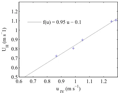
We also estimated discharge from the H-ADCP data based on the IVM approach (Le Coz et al., 2008). We compute dis-charge by regressing the H-ADCP index velocity with cross-section averaged velocity, yielding discharge after multiply-ing it with the cross-section area. We used the more represen-tative and accurate part of the HADCP velocity profile data

IV

Fig. 9. IVM rating fitted by linear regression over five boat surveys

covering the whole channel width.

fromβ= 0.5 to 0.7 for computing the index velocity. The IVM discharge was computed as:

QIVM=f (u)A (10)

whereuis the index velocity andAis river cross sectional area calculated from the bathymetry profile and the measured water level. The reference mean velocityUH at the H-ADCP

section is obtained from: UH=Qref/A, hereinQrefis the

reference discharge measured by ADCP. The linear regres-sion over five ADCP surveys covering the whole channel cross section yieldedf (u)=0.95u−0.1 (Fig. 9).

3.4 Stage-discharge relation

To investigate the degree in which discharge at Melak sta-tion can be captured by a rating curve, Jones’ formula was applied, which reads:

Q=Qkin

1+ 1 cS0

∂h ∂t

1/2

(11) whereQkinis the kinematic or equilibrium discharge, cis the wave celerity,S0is the bed slope, and∂h/∂tis the rate of water level change in timet all measured at the same lo-cation (Petersen-Overleir, 2006). The celerity c was esti-mated fromc=dQ

dA=B −1dQ

dh (Henderson, 1966) based on the steady flow rating curve obtained for Melak. Herein,Ais river cross sectional area andBis river width. The bed slope of 10−4was estimated from the Mahakam River bed level profile derived from SRTM data by van Gerven and Hoitink (2009).Qkinwas calculated using the Manning formula:

Qkin= 1 nS

1/2 0 AR

2/3 ₍₁₂₎

Table 1. Evaluation of channel conditions at Melak station to

esti-mate the Manning coefficient.

Factor (index) Description (value)

Additive factors

−Material involved (n₀) Earth (0.02) −Degree of irregularity (n₁) Minor (0.005) −Var. in location of thalweg (n₂) Gradual (0.00) −Effect of obstruction (n₃) Negligible (0.00) −Riparian vegetation (n₄) Medium (0.01) Multiplicative factors

−Degree of meandering (m) Appreciable (1.15)

n=(n₀+n₁+n₂+n₃+n₄)m=0.04025

perimeter of the river cross-section. The Manning coefficient was estimated based on an evaluation of the river geometry and composition, following a standard empirical technique provided by Gore (2006). The details of channel evaluation to determinenare presented in Table 1.

We used the rating curve discharge estimate from Eq. (11) in most of the discussion in Sect. 4. Equation (12), how-ever, is used with the assumption that the river reach (Fig. 2, top panel) has a uniform channel geometry. The presence of the jetty and boats resulted in irregularity in the channel cross-section (Fig. 2, bottom panel) locally at the station. In the original version of the Jones formula, the discharge taken from the currently available steady flow rating curve (Q0) is used instead of using Eq. (12). For a comparison, we also computed discharge using the Jones’ formula based onQ0.

4 Results and discussion

Table 2 shows the validation results. Discharge estimates obtained by applying the method by Sassi et al. (2011) and IVM differed less than 5 % from the accurate estimates ob-tained from the boat surveys. Figure 10 shows time-series of the absolute and relative difference between QDSM and QIVM, which indicate that the validation results represent the medium to high flows well. During low flows,QDSM and QIVM can deviate much more, both in a relative and in an absolute sense. Unfortunately, a planned validation survey during the low flow condition was cancelled due to technical problems, which could have shed more light on the validity of the low-flow discharge estimates. Regarding high flows, the larger difference betweenQDSMandQIVMcould be due to the fact that the H-ADCP is monitoring flow at a rela-tive depth that changes with the river stage, which challenges the constancy of the conversion factor to calculate discharge from the index velocity. The IVM is heavily dependent on the degree in which the velocity measurements within the

Table 2. Results of the three validation surveys of the DSM and

the IVM methods. QBSdenotes the discharge calculated from the boat survey, which can be considered truth.

Val. Q_BS Q_DSM Q_IVM Q_DSM/Q_BS Q_IVM/Q_BS

1 1823 1875 1889 1.03 1.04

2 2438 2439 2465 1.00 1.01

3 2387 2417 2382 1.01 1.00

H-ADCP range unambiguously covary with the cross-section averaged velocity and on the degree in which the calibration surveys cover extreme conditions. The obtained results high-light the merits of applying the more elaborate procedure ad-vocated by Hoitink et al. (2009) and Sassi et al. (2011) par-ticularly in a remote poorly-gauged area. Compared to the IVM, the DSM is more physically based, which provides a better resilience to cope with a lack of discharge measure-ments during high flows and low flows. Even in the case of an equal performance, as established from a small number of validation surveys in our study, the DSM is to be preferred because the IVM can be right for the wrong reasons. The IVM is only to be preferred over the DSM when calibration data cover the full range of conditions and there are no iner-tial effects, which create a time lag between local flow veloc-ity and cross-section averaged flow velocveloc-ity.

−1000 0

∆

Q (m

3 s

−

02−Apr−2008 11−Jul−2008 19−Oct−2008 27−Jan−2009 07−May−2009 15−Aug−2009 −0.5

0 0.5

∆

Q/Q (−)

Fig. 10. Continuous series of discharge estimates derived from H-ADCP data with the DSM and the IVM. Central and bottom panels offer a

comparison between DSM and the IVM to convert H-ADCP data to discharge, where1Q=QDSM−QIVM.

0 1000 2000 3000 4000

2 4 6 8 10

Q (m3 s−1)

h (m)

H−ADCP (IVM) H−ADCP (DSM) Rating curve

Fig. 11. Water stage and discharge estimates at Melak station,

ob-tained from a rating curve (Jones’ formula) and from H-ADCP mea-surements. Water stage is with respect to the position of a pressure gauge about 9 m from the deepest part of the river cross-section.

Mahakam delta. At low discharges in August 2009, the tidal signal is clearly visible in the discharge series. Due to the flat terrain of the middle and lower Mahakam, tidal energy propagates up to the Mahakam lakes area, where much of the tidal energy is dissipated. Subharmonics such as the MSf, an oceanographic term for the fortnightly constituent of the tide created by nonlinear interaction of the tides induced by the Moon and the Sun with the river discharge, may extend be-yond the lakes region. However, this effect cannot be readily isolated from river discharge variation as discharge variation features fortnightly variation both in the presence and in ab-sence of a tidal influence.

0 500 1000 1500 2000 2500 3000 4

5 6 7 8 9 10

Q (m3 s−1)

h (m)

H−ADCP (IVM) H−ADCP (DSM) Rating curve

28 June 24 May

Fig. 12. Water stage versus discharge for the period between 24 May–28 June 2008. Multiple loops and discharge oscillations in-dicate variable backwater effects also occurred within the hysteresis loop.

19−May−2008 29−May−2008 08−Jun−2008 0 1000 2000 3000 Q (m

3 s

− 1) 0 2 4 6 8 10 h (m)

29−Oct−2008 08−Nov−2008 18−Nov−2008 0

1000 2000 3000

Q (m

3 s

− 1) 0 2 4 6 8 10 h (m) Q Melak h Melak h Lake Jempang h Muara Kaman

Fig. 13. Water stage and discharge during lake emptying (top) and

during lake filling (bottom). Muara Kaman, where the tidal signal was observed during most of the measurement period, is located downstream of the Mahakam lakes area about 170 km from Melak.

velocity. Figure 13 illustrates the lake emptying and lake fill-ing influencfill-ing water levels and discharge upstream. At the start of lake emptying, when the lake level was still high, water stage in Melak was relatively high for a relatively low discharge. When the lake level dropped, the backwater effect was reduced and discharge increased while water stage kept decreasing until the point that discharge was sufficiently high to make water stage follow the trend in the discharge time-series. The opposite mechanism took place during lake fill-ing as shown in Fig. 13 (bottom panel). Water stage records downstream of the Mahakam lake area (Muara Kaman) indi-cate that some peaks of water level were shaved by the lake filling and emptying mechanism.

The discharge obtained from the stage-discharge relation using Jones formula is merely a rough estimate of discharge at Melak station, indicating the range of discharge variation. It did not capture the detailed discharge dynamics as revealed by the H-ADCP measurements. This can be related to a wide variety of reasons. The Froude number takes a value around 0.01, which likely indicates the inertial term in the momen-tum equation to be negligible. A non-dimensional version of the St. Venant equations directly shows that the inertial terms drop out for small values of the Froude number (Pearson, 1989). The key assumption used to derive the Jones formula is the applicability of the kinematic wave equation to deal

500 1000 1500 2000 2500 3000 3500 500 1000 1500 2000 2500 3000 3500 Q

J−Qsteady RC (m 3

s−1) Q J−Qkinematic

(m

3 s

−

1 )

Fig. 14. Comparison of discharge estimates obtained using the

Jones formula based onQkin(uniform channel geometry assump-tion) and those based onQ0(discharge taken from the steady flow rating curveQ0=125.98×(h+1.5)1.256) for the whole observa-tion period. The small deviaobserva-tion confirms that the two approaches yield similar results. Only during peak discharges, the use ofQ0 instead ofQkin can result in slightly different rating curve-based estimates of the discharge.

ventional boat-mounted ADCP measurements were periodi-cally taken to establish water discharge through the cross sec-tion. We followed a recently developed semi-deterministic, semi-stochastic method (DSM) to convert the H-ADCP to discharge, and compared the results with those obtained from the index-velocity method (IVM) and a rating curve model. The DSM method was found to be comparable with the IVM, the difference with discharge estimates from the boat-mounted ADCP surveys was less than 5 % based on three validation surveys. The continuous time-series of dis-charge showed that the validation data were representative for medium to high flows. A stage-discharge model based on Jones’s formula captured only a small portion of the dis-charge dynamics, which was attributed to the invalidity of the kinematic wave assumption due to backwater effects. A dis-charge range of about 2000 m3s−1was established for a par-ticular stage in the recorded discharge series, which is about 60 % of the peak discharge and therefore exceptionally large. The large range of discharge occurring for a given stage was attributed to multiple backwater effects from lakes and tribu-taries, floodplain impacts and effects of river-tide interaction, which generate subharmonics that cannot readily be isolated from river discharge oscillations.

Acknowledgements. This research has been supported by the Netherlands organisation for scientific research, under grant number WT 76-268. The help from Fajar Setiawan and Unggul Handoko (LIPI – Research Centre for Limnology) and David Vermaas (Wageningen University) in data collection is gratefully acknowledged. The authors appreciate comments and suggestions from the three reviewers that helped improve the manuscript.

Edited by: G. Di Baldassarre

References

Beven, K. J.: Rainfall-runoff modelling: the primer, John Wiley & Sons, Chichester, England, 2001.

Buschman, F. A., Hoitink, A. J. F., van der Vegt, M., and Hoekstra, P.: Subtidal water level variation controlled by river flow and tides, Water Resour. Res, 45, 1–12, doi:10.1029/2009WR008167, 2009.

Godin, G. and Mart´ınez, A.: Numerical experiments to investigate the effects of quadratic friction on the propagation of tides in a channel, Cont. Shelf Res., 14, 723–748, 1994.

Gordon, R. L.: Acoustic measurement of river discharge, J. Hy-draul. Eng., 115, 925–936, 1989.

Gore, J. A.: Methods in Stream Ecology, chap. Discharge Measure-ments and Streamflow Analysis, Academic Press, 51–77, 2006. Henderson, F. M.: Open channel flow, Prentice Hall, 544 pp., 1966. Herschy, R. W.: Streamflow Measurement, Taylor & Francis,

Lon-don and New York, 3rd Edn., 2009.

Hidayat, Hoekman, D. H., Vissers, M. A. M., and Hoitink, A. J. F.: Combining ALOS-PALSAR imagery with field water level mea-surements for flood mapping of a tropical floodplain, Proceed-ings of the International Symposium on LIDAR and Radar Map-ping: Technologies and Applications, Nanjing, China, in press, 2011.

Hoitink, A. J. F., Buschman, F. A., and Vermeulen, B.: Continuous measurements of discharge from a horizontal acoustic Doppler current profiler in a tidal river, Water Resour. Res, 45, 1–13, doi:10.1029/2009WR007791, 2009.

Jones, B. E.: A method of correcting river discharge for a changing stage, US Geological Survey Water Supply Paper, 375-E, 117-130, 1916.

Koussis, A. D.: Comment on “A praxis-oriented perspective of streamflow inference from stage observations – the method of Dottori et al. (2009) and the alternative of the Jones Formula, with the kinematic wave celerity computed on the looped rating curve” by Koussis (2009), Hydrol. Earth Syst. Sci., 14, 1093– 1097, doi:10.5194/hess-14-1093-2010, 2010.

Lamberti, P. and Pilati, S.: Quasi-kinematic flood wave propaga-tion, Meccanica, 25, 107–114, 1990.

Le Coz, J., Pierrefeu, G., and Paquier, A.: Evaluation of river dis-charges monitored by a fixed side-looking Doppler profiler, Wa-ter Resour. Res., 44, 1–13, doi:10.1029/2008WR006967, 2008. McMillan, H., Freer, J., Pappenberger, F., Krueger, T., and Clark,

M.: Impacts of uncertain river flow data on rainfall-runoff model calibration and discharge predictions, Hydrol. Process., 24, 1270–1284, doi:10.1002/hyp.7587, 2010.

Moore, S. A., Le Coz, J., Hurther, D., and Paquier, A.: Backscat-tered intensity profiles from horizontal acoustic Doppler cur-rent profilers, in River Flow 2010, Bundesanstalt fur Wasserbau, Braunschweig, Germany, 1693–1700, 2010.

15, doi:10.1029/2008WR006970, 2008.

Pearson, C. P.: One-dimensional flow over a plane: Criteria for kinematic wave modelling, J. Hydrol., 111, 39–48, 1989. Perumal, M. and Ranga Raju, K. G.: Approximate

convection-diffusion equations, J. Hydrol. Eng., 4, 160–164, 1999. Perumal, M., Shrestha, K. B., and Chaube, U. C.: Reproduction of

Hysteresis in Rating Curves, J. Hydrol. Eng.-ASCE, 130, 870-878, 2004.

Petersen-Overleir, A.: Modelling stage-discharge relationships af-fected by hysteresis using the Jones formula and nonlinear re-gression, Hydrol. Sci. J., 51, 365–388, 2006.

Petersen-Overleir, A. and Reitan, T.: Bayesian analysis of stage-fall-discharge models for gauging stations affected by variable backwater, Hydrol. Process., 23, 3057–3074, doi:10.1002/hyp.7417, 2009.

Sassi, M. G., Hoitink, A. J. F., Vermeulen, B., and Hidayat: Dis-charge estimation from H-ADCP measurements in a tidal river subject to sidewall effects and a mobile bed, Water Resour. Res., 47, W06504, 1–14, doi:10.1029/2010WR009972, 2011.

Schmidt, A. R.: Analysis of stage-discharge relations for open-channel flows and their associated uncertainties, PhD the-sis,University of Illinois, available at: https://netfiles.uiuc.edu/ aschmidt/www/ARS Thesis/ARS Thesis.htm (last access: 9 Au-gust 2011), 2002.

Simpson, M. R. and Bland, R.: Methods for accurate estimation of net discharge in a tidal channel, IEEE J. Oceanic Eng, 25, 437– 445, 2000.

Tsai, C. W.: Flood routing in mild-sloped rivers – wave characteris-tics and downstream backwater effect, J. Hydrol., 308, 151–167, doi:10.1016/j.jhydrol.2004.10.027, 2005.

van Gerven, L. P. A. and Hoitink, A. J. F.: Analysis of river plan-form geometry with wavelets: application to the Mahakam River reveals geographical zoning, in: Proceedings of RCEM, 2009. Yen, B. C. and Tsai, C. W. S.: On noninertia wave versus diffusion