www.hydrol-earth-syst-sci.net/15/1081/2011/ doi:10.5194/hess-15-1081-2011
© Author(s) 2011. CC Attribution 3.0 License.
Earth System
Sciences
Assessment of a vertical high-resolution
distributed-temperature-sensing system in a shallow thermohaline environment
F. Su´arez1, J. E. Aravena2, M. B. Hausner3, A. E. Childress2, and S. W. Tyler1 1Department of Geological Sciences and Engineering, University of Nevada, Reno, USA 2Department of Civil and Environmental Engineering, University of Nevada, Reno, USA 3Graduate Program of Hydrologic Sciences, University of Nevada, Reno, USA
Received: 28 November 2010 – Published in Hydrol. Earth Syst. Sci. Discuss.: 5 January 2011 Revised: 25 March 2011 – Accepted: 26 March 2011 – Published: 30 March 2011
Abstract. In shallow thermohaline-driven lakes it is im-portant to measure temperature on fine spatial and tempo-ral scales to detect stratification or different hydrodynamic regimes. Raman spectra distributed temperature sensing (DTS) is an approach available to provide high spatial and temporal temperature resolution. A vertical high-resolution DTS system was constructed to overcome the problems of typical methods used in the past, i.e., without disturbing the water column, and with resistance to corrosive environments. This paper describes a method to quantitatively assess ac-curacy, precision and other limitations of DTS systems to fully utilize the capacity of this technology, with a focus on vertical high-resolution to measure temperatures in shallow thermohaline environments. It also presents a new method to manually calibrate temperatures along the optical fiber achieving significant improved resolution. The vertical high-resolution DTS system is used to monitor the thermal be-havior of a salt-gradient solar pond, which is an engineered shallow thermohaline system that allows collection and stor-age of solar energy for a long period of time. The vertical high-resolution DTS system monitors the temperature pro-file each 1.1 cm vertically and in time averages as small as 10 s. Temperature resolution as low as 0.035◦C is obtained when the data are collected at 5-min intervals.
Correspondence to: F. Su´arez (suarezf@unr.edu)
1 Introduction
Temperature fluctuations are a major driver of changes in nat-ural and managed aquatic systems (Rosenzweig et al., 2007). In thermohaline aquatic environments such as estuaries or saline lakes, it is important to measure temperature on fine spatial and temporal scales to detect stratification or different hydrodynamic regimes. Spatial variability in shallow ther-mohaline systems can occur on vertical scales of centime-ters and temporal variability occurs on time scales ranging from minutes to months, or even years (Anati and Stiller, 1991; Lorke et al., 2004; Lu et al., 2004; Kurt and Ozkay-mak, 2006). Measuring temperature at these scales, espe-cially when diurnal cycles need to be recorded over a long time period, can be difficult because of the cost involved (Branco et al., 2005) and other practical limitations, such as placing multiple sensors in a limited space. Multiple sen-sors need to be independently calibrated and may be subject to different intensities of drift in thermohaline environments (Bergman et al., 1985).
Fiber-optic distributed temperature sensing (DTS) is an approach available to provide coverage in both space and time that can be used to continuously monitor real-time data in different environments. It was first developed in the 1980s (Dakin et al., 1985) and used in the oil and gas industry dur-ing the 1990s and early 2000s (Kersey, 2000); only since 2006 has it been widely used in hydrologic applications (Selker et al., 2006; Westhoff et al., 2007; Moffett et al., 2008; Tyler et al., 2009; Vogt et al., 2010). DTS technol-ogy uses Raman spectra scattering in a fiber-optic cable to measure temperatures along the cable length (this is referred to as the temperature trace). The ratio between the anti-Stokes and anti-Stokes wavelengths of the Raman scattering is used to estimate the temperature along the fiber, and the loca-tion of the temperature measurement along the cable is cal-culated using the travel times of the incident and scattered lights. A detailed description of the theoretical basis of DTS systems is out of the scope of this work and can be found elsewhere (Rogers, 1999; Selker et al., 2006). Commonly available DTS systems can achieve a temperature resolution as fine as 0.01◦C (using 30-min integration-time intervals) with typical spatial and temporal resolutions of 1–2 m and 10–60 s, respectively, for cables up to 10 km (Selker et al., 2006). However, there are hydrologic environments such as shallow (<2 m deep) lakes or ponds where thermal obser-vations at smaller vertical scales are required (Losordo and Piedrahita, 1991; Branco and Torgersen, 2009; Su´arez et al., 2010a). This has resulted in the development of vertical high-resolution DTS systems.
The pioneering of a vertical high-resolution DTS system for hydrologic applications was presented by Selker et al. (2006). They monitored temperatures on a glacier and in a lake using an optical fiber wrapped around a 75 mm diame-ter 2 m length polyvinyl chloride (PVC) pole. Two platinum resistance thermistors (PT100), located at the top and bot-tom of the pole, were used to calibrate the temperature mea-surements along the optical fiber. This DTS system achieved a vertical spatial sampling resolution of 0.4 cm and a temper-ature resolution of 0.05◦C when 2 min integration intervals were used. Radiative heating on the pole had a profound impact on the air measurements above the glacier (Huwald et al., 2009). In the lake, where the water column was strongly mixed by the presence of waves during overcast con-ditions, radiative heating of the DTS pole was not observed. As the main purpose of the work performed by Selker et al. (2006) was to demonstrate the potential of DTS methods, only limited efforts were made to quantitatively assess the limitations of their DTS system. For example, having only two points of independent temperature measurements along the DTS pole may result in lower temperature accuracy along the optical fiber than that achieved with longer sections of cable at known temperature. Recently, Vogt et al. (2010) constructed a high-resolution DTS vertical temperature pro-filer to estimate seepage rates in a losing reach of a river. A fiber-optic cable was wrapped around a 51 mm diameter
1.9 m length PVC piezometer tube. The calibration of their DTS system was performed in the laboratory before field in-stallation with two reference sections at two known tempera-tures. According to their manufacturer specifications, a tem-perature resolution of at least 0.11◦C should be achieved for cables shorter than 2 km when 10 min integration intervals were used. Although they were able to study groundwater and surface water interactions, deviations occurred due to calibration and signal noise of the DTS as well as solar ra-diation heating the DTS pole when the river stage was very low.
With their spatial and temporal resolution, DTS methods offer significant advantages over traditional measurement systems in natural or managed thermohaline environments. Fibers are low cost, with no issues of bias or fluid column dis-turbance, and can be made completely non-corroding. Radi-ation effects are similar to traditional sensors (Neilson et al., 2010). Nonetheless, DTS methods have complications and limitations that must be understood and assessed in order to achieve improved resolution. For instance, accuracy and precision of DTS systems depend on the fraction of incident light that is backscattered in the optical fiber and thus, one of the main limitations of DTS systems is low signal strength. Hence, care must be taken to avoid signal strength reduc-tions, and evaluation of accuracy and precision of DTS sys-tems is necessary for each installation. Also, DTS syssys-tems must be calibrated for differential attenuation of the anti-Stokes and anti-Stokes intensities along the cable as well as in-strument sensitivity and drift. Previous DTS investigations in hydrological or environmental applications have never pre-sented the equations that DTS systems use for temperature estimation or temperature calibration. Few investigations in the field of light physics have derived the governing equa-tion for temperature estimaequa-tion along the fiber (Farahani and Gogolla, 1999; Yilmaz and Karlik, 2006), but their notation is inconsistent and some parameters have not been clearly defined. Therefore, temperature estimation (or calibration) in fiber-optic DTS systems still remains unclear.
monitor temperatures in a salt-gradient solar pond (hereafter, the term salt-gradient will be dropped), an engineered shal-low thermohaline system that consists of three distinctive layers (Su´arez et al., 2010b): the upper convective zone, a thin layer of cooler, less salty water; the non-convective zone, which has gradients in temperature and salinity; and the lower convective zone, a layer of high salinity brine (near saturation) where temperatures are the highest. In particu-lar, temperatures collected with electrical conductivity (EC) probes are used to compare the DTS measurements within the solar pond, and the effects of radiative heating on the op-tical fiber are evaluated.
2 Materials and methods
2.1 Vertical high-resolution DTS system
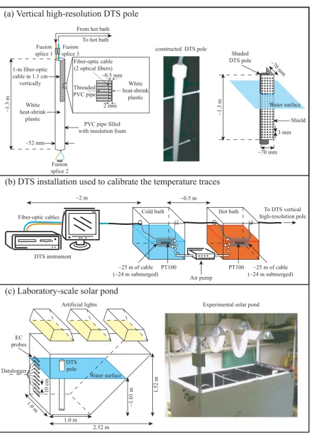
A vertical high-resolution DTS system was constructed con-sisting of a vertical high-resolution pole, a DTS instrument, two water baths at different temperatures (for calibration pur-poses), and a fiber-optic cable that connects all the compo-nents. The total length of the fiber-optic cable was∼400 m, with∼200 m used in the vertical high-resolution DTS pole, ∼50 m used in each bath, and the remainder used to connect the DTS instrument with each component of the system. 2.1.1 Vertical high-resolution DTS pole
A vertical high-resolution DTS pole (Fig. 1a) was con-structed by carefully wrapping a duplex (i.e., two fibers in one cable) multi-mode fiber-optic cable (AFL Telecommu-nications, Spartanburg, SC) around a 51 mm diameter PVC pipe∼1.3 m in length. The geometric characteristics of the fiber-optic cable and the PVC pipe allowed 1 m of cable to occupy 1.1 cm of pipe length. The fiber-optic cable consists of a plastic jacket tube filled with a thixotropic gel and two non-armored optical fibers with core and cladding diameters of 50 and 125 µm, respectively. The cable was secured to the pipe using a white heat-shrink plastic, which is likely to reduce radiative heating. The interior of the PVC pipe was filled with insulating foam to prevent convective heat flow in-side the pipe itself. The result was an easily handled, chem-ically inert, light-weight pole, resistant to the corrosive en-vironment of hot saline water. The two optical fibers were fused at the end of the cable to create a loop of a single ca-ble with both ends connected to the DTS instrument. This allowed access to the entire optical path of the cable via con-nection of the DTS to either end of the fiber.
2.1.2 DTS instrument
The vertical high-resolution DTS pole was connected to a Sensornet Sentinel DTS instrument (Sensornet Ltd., Herth-fordshire, England), which according to the manufacturer,
has a temperature resolution<0.01◦C (60 min integration
in-tervals) and a spatial sampling interval of 1.015 m, when ca-bles shorter than 5 km are used. A four-channel multiplexer was employed to allow the use of single- or double-ended measurements. Single-ended measurements refer to temper-atures estimated from light transmission in only one direction along the fiber. These measurements provide more preci-sion near the instrument and degrade with distance due to the energy loss along the fiber length. Double-ended measure-ments refer to temperatures estimated from light transmis-sion in both directions along the fiber. In double-ended mea-surements, the temperature is estimated using single-ended measurements made from each end of the optical fiber and accounts for spatial variation in the differential attenuation of the anti-Stokes and Stokes signals, which often occurs in damaged or strained fibers. This results in a signal noise more evenly distributed across the entire length of the cable, but uniformly greater than that obtained in a single-ended measurement (Tyler et al., 2009).
2.1.3 Calibration and verification
Here, we present a new method to calibrate temperatures along the fibers for single-ended measurements. We recog-nize that it is also necessary to present a calibration method for double-ended measurements, especially for damaged or strained cables that have spatially variable differential atten-uation. However, because the differential attenuation along the length of our cable was fairly constant and due to the complexity of this method, it is out of the scope of this work and it remains to be a topic that will continue to be addressed in future investigations.
The temperature in an optical fiber can be estimated by (Farahani and Gogolla, 1999; Yilmaz and Karlik, 2006):
T (z) = γ
ln[C] − ln[R(z)] + 1 α z (1)
R(z) = IaS(z)/IS(z) (2)
constructed DTS pole
Shield Shaded
DTS pole ~70 mm
~70 mm 3 mm
~1.3 m
Water surface
~52 mm White heat-shrink
plastic
Fusion splice 2 Fusion splice 1
Fusion splice 3
1-m fiber-optic cable in 1.1 cm
vertically
Threaded PVC pipe
White heat-shrink
plastic Fiber-optic cable
(2 optical fibers) ~0.5 mm
2 mm
~1.3 m
PVC pipe filled with insulation foam From hot bath
To hot bath
(a) Vertical high-resolution DTS pole
(b) DTS installation used to calibrate the temperature traces
DTS instrument
To DTS vertical high-resolution pole
Cold bath Hot bath
~0.5 m
~25 m of cable (~24 m submerged) ~25 m of cable
(~24 m submerged) ~2 m
Air pump
PT100 PT100
Fiber-optic cables
(c) Laboratory-scale solar pond
10 cm
EC probes
DTS pole
2.52 m
1.52 m
1.0 m
~1.01 m
Water surface Datalogger
Artificial lights
1.0 m
[image:4.595.72.525.57.694.2]Experimental solar pond
generally assumes that the constantγis known ahead of time and thus, the calibration requires two points (or sections) of known temperature to determine the constants 1α andC. This calibration method has been widely used in previous hydrologic investigations (Selker et al., 2006; Westhoff et al., 2007; Tyler et al., 2009). Second, temperatures can be cali-brated manually using Eq. (1) (this is referred to as extended calibration). This calibration method assumes that the con-stants1α,γ andCare not known ahead of time. As a result, this calibration method requires three points (or sections) of known temperature. Two of these points can be at the same temperature and the other one at a different temperature. In the extended calibration method, two points held at the same temperature on the optical fiber are used to calculate1α. If z1andz2are the positions of these points, Eq. (1) yields: 1α = (ln [R (z1)] − ln [R (z2)])
(z1 −z2)
(3) Once1α is known, the values of C and γ are calculated using Eq. (1) at two points on the fiber held at different tem-peratures:
ln[C] = (ln [R (z1)] −1α z1) T (z1) T (z1) −T (z3)
...
−(ln[R (z3)] −1α z3) T (z) T (z1) −T (z3)
(4) γ = (ln[C] − ln [R (z1)] +1α z1) T (z1) (5) wherez3is the position of a point on the fiber that has differ-ent temperature than that at positionsz1orz2. When sections (instead of points) of known temperature are used to estimate the calibration parameters, the differential attenuation is cal-culated using the mean value of the1αof contiguous points within the section, thenCandγ are estimated using Eqs. (4) and (5). After the values of1α,Candγ are known, Eq. (1) is used to calculate the temperatures along the entire fiber. Calibration parameters (1α, C andγ) are recalculated for each time-step and are assumed to be uniform over the entire fiber length.
Two water baths were used as known-temperature refer-ence sections to calibrate and verify the temperature read-ings of the DTS system (Fig. 1b). The first 25 m of cable were placed in a room-temperature water bath (cold bath) and were used to calibrate the temperature along the fiber. A four-wire 100-Ohm platinum resistance thermistor (PT100, ±0.1◦C) was positioned in the cold bath. The next 25 m of cable were placed in a microprocessor-controlled water bath (Precision 280, Thermo Electron Corporation, Waltham, MA) at a constant temperature of∼60◦C (hot bath). A sec-ond PT100 thermistor (±0.1◦C) was placed in the hot bath to verify the calibrated DTS readings. Air was circulated in both water baths to insure well mixed, isothermal condi-tions. The PT100 thermistors were previously calibrated us-ing an NIST-traceable VWR thermometer (±0.05◦C; Con-trol Company, Friendswood, TX).
2.1.4 Resolution and repeatability
Spatial resolution is typically defined by DTS manufacturers as the length of cable required to show 80% of the temper-ature change between two known tempertemper-atures. To evaluate the spatial resolution of the DTS system, the step change in temperature between the cold and hot baths was analyzed. To evaluate the temporal resolution, a location on the optical fiber was monitored. When a fast and significant change in temperature occurred, the response time of the system was recorded and the temporal resolution was determined.
Repeatability refers to the agreements between successive measurements carried out under the same conditions. Spa-tial repeatability was quantified during a single trace by the standard deviation of consecutive temperature measurements over a given length of fiber that is at uniform temperature (Tyler et al., 2009). Temporal repeatability was quantified in a single point of the trace that was at a constant temperature by calculating the standard deviation of consecutive temper-ature measurements over a given time period.
2.1.5 Single- and double-ended measurements
The effect of single- and double-ended measurements on the temperature measurements was evaluated by comparing the temperature readings in the hot bath. In addition, the effect of temporal integration was also studied. Different combina-tions of measurements (single- and double-ended) and inte-gration times were evaluated.
2.2 Evaluation of the vertical high-resolution DTS system in an experimental solar pond
0 50 100 150 200 250 300 350 400 10
20 30 40 50 60 70
Distance along fiber optic [m]
T
emperature [ºC]
2000 2500 3000 3500 4000 4500 5000
Scattered amplitude
Stokes anti-Stokes
25 Mar 2009 - 11:46 am
25 Mar 2009 - 11:46 am 10 Mar 2009 - 08:24 am
(a)
(b)
Hot bath
Cold bath
LCZ NCZ
UCZ Air
Vertical high-resolution DTS pole
Fusion splice 1
Fusion splice 3 Fusion
splice 2
Hot bath
Cold bath
0 50 100 150 200 250 300 350 400
Vertical high-resolution DTS pole
LCZ: lower convective zone NCZ: non-convective zone UCZ: upper convective zone
z1 z3 z2
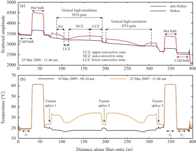
Fig. 2. (a) Typical Raman-scattering traces obtained during the experiment show the impact of temperature on the anti-Stokes and Stokes signals. Locations of the system components (cold and hot baths, vertical high-resolution DTS pole) are also shown. (b) Typical temperature traces measured during the experiment (obtained using the manufacturer-internal calibration method). The black line was obtained at the beginning of the experiment and the orange line was obtained after 15 days.
The lower 50 cm of the solar pond (i.e., the lower convec-tive zone) were filled with a 20 wt% sodium chloride (NaCl) solution. Then, eight layers of successively lower concentra-tions were added up to an elevation of 90 cm measured from the bottom of the solar pond (i.e., the non-convective zone). Each layer had a NaCl concentration that was 2.2% lower than that of the previous layer. The final layer (i.e., the up-per convective zone) was filled with tap water. The average water level in the solar pond was 101 cm (measured from the bottom), but the actual level varied from 98 to 103 cm due to evaporation and freshwater resupply. The average water level was used to calculate depths within the solar pond through-out the experiment (regardless that the true water level var-ied). The solar pond was covered tightly and allowed to sit for three days after filling. Then, the pond was typically ex-posed to the artificial lights 12 h per day (from 06:00 a.m. to 06:00 p.m. with the exception of the first day that was from 09:00 a.m. to 06:00 p.m.) and its thermal response was mon-itored using 5 min integration-time intervals.
In a separate investigation to assess the impact of radia-tive heating on the DTS pole, the lights over the pond were operated continuously. When the solar pond was close to
thermal steady state, the DTS pole was shaded using a white expanded-foam PVC shield (Fig. 1a). Holes were made in the shield to allow air (above the water surface) and water to move across it. The DTS pole was covered for approximately 60 min until a new steady state was reached. After this, the DTS pole was uncovered and temperatures were recorded us-ing 10 s integration-time intervals until the initial value was reached.
3 Results and discussion
3.1 Vertical high-resolution DTS system
[image:6.595.98.495.63.367.2]cable was fused. The temperature traces are symmetrical be-cause the two fibers within the cable were fused at the end (fusion splice 2) to create a single loop. Figure 2 also shows how the temperature along the optical fiber affects the anti-Stokes and anti-Stokes signals. As expected, the anti-anti-Stokes sig-nal is strongly dependent on the temperature along the fiber while the Stokes signal is weakly dependent on the tempera-ture.
3.1.1 Calibration and verification
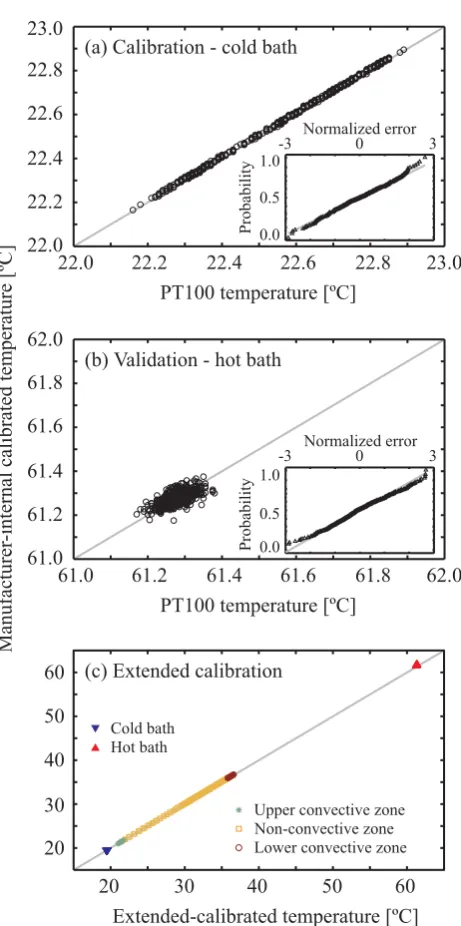
Figure 3a shows a comparison of the temperatures measured in the cold bath by the PT100 and by the DTS system. The DTS temperatures were calibrated using the manufacturer-internal calibration. These temperatures are expected to be equal because the DTS instrument uses the temperature sured in the cold-bath PT100 to correct the temperature mea-surements along the entire optical fiber. A normal probabil-ity plot (inset of Fig. 3a) shows that the difference between the DTS and PT100 temperatures follows a standard normal distribution (i.e.,∼N (0,1)). Thus, these temperature differ-ences are verified to be independent and could be considered as random noise with 95% confidence (Box et al., 2008).
The manufacturer-internal-calibrated DTS readings were verified by comparing the DTS and the PT100 measurements in the hot bath, as shown in Fig. 3b. The temperatures of both instruments are in agreement, although their differences have more variability than those measured in the cold bath. How-ever, a normal probability plot shows that these temperature differences are also ∼N (0,1). Thus, random noise in the DTS system is the main reason for the observed differences, with a 5% significance level (Box et al., 2008). Statistically, the DTS and the thermistor measure the same temperature, verifying the readings of the DTS system.
To illustrate the extended calibration method, single-ended traces of the anti-Stokes and Stokes intensities were used to estimate the temperatures along the optical fiber. These temperatures were compared to the manufacturer-internal-calibrated temperatures. The mean value of the 1α was calculated from two sections on the optical fiber held at the same temperature (between 10 and 25 m and between 370 and 385 m, in the cold bath at∼19.6◦C, as shown in Fig. 2). The values ofC andγ were calculated from two points on the fiber held at different temperatures (z1= 17.5 m at∼19.6◦C in the cold bath andz3= 347.5 m at∼61.5◦C in the hot bath). Figure 3c compares manufacturer-internal-and extended-calibrated temperatures within the solar pond. Generally, these calibrated temperatures differ in less than 0.1◦C in the solar pond. The root mean square error (RMSE) of the points of known temperature along the cable was used to determine the goodness of the agreement between these calibrations. The extended-calibrated temperatures (RMSE = 0.05◦C) are closer than the manufacturer-internal-calibrated temperatures (RMSE = 0.25◦C) to the indepen-dent measures of temperature of the baths. This occurred
Upper convective zone Non-convective zone Lower convective zone Cold bath
Hot bath
22.0 22.2 22.4 22.6 22.8 23.0
22.0 22.2 22.4 22.6 22.8 23.0
61.0 61.2 61.4 61.6 61.8 62.0
61.0 61.2 61.4 61.6 61.8 62.0
20 30 40 50 60
20 30 40 60
50
Extended-calibrated temperature [ºC]
Manufacturer
-internal calibrated temperature [ºC]
PT100 temperature [ºC]
-3 0 3
0.0 0.5 1.0
Probability
Normalized error
-3 0 3
0.0 0.5 1.0
Probability
Normalized error
(c) Extended calibration (b) Validation - hot bath (a) Calibration - cold bath
PT100 temperature [ºC]
Fig. 3. (a) The DTS system is calibrated by comparing the PT100 temperature measurements with the DTS manufacturer-internal cal-ibrated temperatures in the cold bath. (b) The DTS system is vali-dated in the hot bath. (c) Extended- and manufacturer-internal cali-brated temperatures are compared.
because manufacturer-internal-calibrated temperatures were estimated by varying two calibration parameters (1αandC), while in the extended-calibrated temperatures three calibra-tion parameters (1α,Candγ) were allowed to vary. Thus, manual post-processed data resulted in a more robust and us-able data set.
[image:7.595.313.544.54.518.2]Table 1. Sensitivity analysis of the extended calibration for dif-ferent lengths (L) of the calibration sections. RMSE andσ cor-respond to the root mean square error and the standard deviation of the extended-calibrated temperatures in the known-temperature sections.
L RMSE σ
[m] [◦C] [◦C] 1 2.077 0.051 5 1.532 0.044 10 0.556 0.038
of the selection ofz1 andz3on quality of the calibration is negligible compared to the effect of the length of the known-temperature section (data not shown). Table 1 show that both the RMSE and the standard deviation of the extended-calibrated temperatures in the calibration baths are reduced as the length of the calibration section is increased. Thus, longer calibration sections are recommended for improved temperature resolution.
3.1.2 Resolution and repeatability
The spatial resolution was evaluated using the step change in temperature between the cold and hot baths. Utilizing 15 days of data (4495 temperature traces), it was found that the mean spatial resolution of the DTS system was 2.056±0.047 m, which is twice that reported by the man-ufacturer. The results obtained here and in a previous study (Tyler et al., 2009) suggest that spatial resolution is at least two times the sampling resolution of the instrument. The temporal resolution of the high-resolution DTS pole was evaluated at∼1 cm above the air-water interface. An integra-tion time of 10 s was utilized. Before the lights were turned on, a constant temperature of 24.223±0.096◦C was
moni-tored. After the lights were turned on, a significant and fast change in temperature (>4◦C in less than 5 min) was
ob-served. The DTS system took less than 40 s to register an increase in temperature larger than 2σ= 0.192◦C. Thus, the temporal resolution of the DTS system was∼40 s with 95% confidence.
Spatial repeatability was quantified during a single trace in the hot bath. The average temperature was 61.429 ± 0.014◦C. This is a very good spatial repeatability that is much better than that obtained in previously reported DTS experiments (Tyler et al., 2008, 2009). Temporal repeatabil-ity was also evaluated in the hot bath. The PT100 reported an average temperature of 61.333±0.120◦C, while that re-ported by DTS system was 61.410±0.121◦C. This suggests that actual variability of the hot bath controls the repeatabil-ity of the DTS measurement.
Table 2. Comparison between single-ended (SE) and double-ended (DE) measurements in the hot bath (obtained using the manufacturer-internal calibration method). T is average tempera-ture andσis standard deviation.
Integration time TSE σSE TDE σDE [s] [◦C] [◦C] [◦C] [◦C] 20 61.419 0.103 61.322 0.112 120 61.612 0.046 61.321 0.069 300 61.618 0.035 61.261 0.055
3.1.3 Single- and double-ended measurements
Selection of single- or double-ended measurements needs to be analyzed because it can result in different degrees of accuracy and temperature resolution. While single-ended measurements provide more precision near the instrument, double-ended measurements allow the users to accurately de-rive temperatures from fibers with spatial variation in the dif-ferential attenuation of the backscattered signals, which typ-ically occurs in damaged or strained fibers.
As shown in Table 2, as the integration time increases the standard deviations of both single- and double-ended measurements decrease. For all the integration times, single-ended measurements show smaller standard deviation than double-ended measurements. An integration time of 300 s showed spatial repeatability (standard deviations) of 0.035 and 0.055◦C in the hot bath for single- and
As a result, the expected decrease in standard deviation due to increasing averaging time is also smaller.
3.2 Evaluation of the vertical high-resolution DTS system in an experimental solar pond
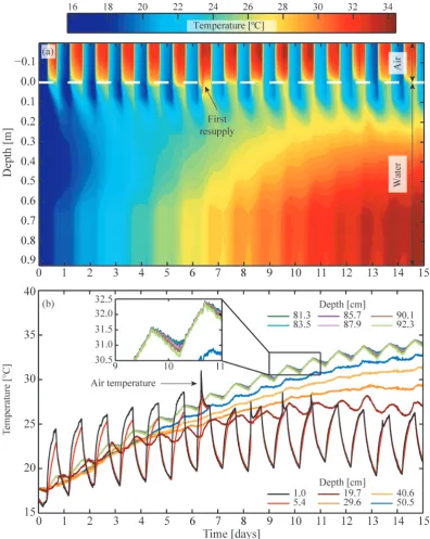
The thermal evolution of the water column and the air above it is presented in Fig. 4a. The night surface cooling, the non-convective zone stratification, and the warming of the lower convective zone are observed at high spatial and temporal resolutions. To the best of our knowledge, this is the first time that temperatures have been reported at such high spatial and temporal resolution in solar ponds (Lu et al., 2004; Kurt and Ozkaymak, 2006). This spatial and temporal resolution of the temperature observations is not only a tool for monitoring temperatures at near real-time but also could become a tool for decision-making. For instance, at the beginning of the experiment, no water was added to the surface of the pond and evaporation decreased the water level. After one week, the DTS system showed air temperatures at more than 5 cm depth; for this reason it was decided to resupply freshwater at the surface of the pond. The timing of the first resupply is clearly observed in Fig. 4a.
Figure 4b shows the thermal evolution at different depths within the solar pond. It can be seen that during the first days of the experiment, the upper convective zone (red and black lines) is stratified during the day and completely mixed during the night. After one week, the upper convective zone is always completely mixed. Figure 4b also shows that the non-convective zone strongly stratifies and that temperatures in the middle of this zone (orange and gold lines) are less affected by daily fluctuations. The close-up in Fig. 4b shows that the lower convective zone is completely mixed during the day but stratified at night because heat is lost through the non-convective zone as well as through the bottom and sides of the experimental solar pond. These heat losses can be easily assessed using the DTS system (e.g., by evaluating the thermal gradient measured near the bottom). For a detailed interpretation of the physics observed in this experiment, the reader is referred to the work of Su´arez et al. (2010c).
Figure 5 shows the temperature profiles using the DTS sys-tem and using EC probes for different days of the experiment. The initial design of the experiment located the interface be-tween the non-convective and the lower convective zones at 0.5 m depth. On the morning of 6 March 2009, only the lower convective zone of the solar pond was filled. At this time, the temperature profile measured with the DTS system showed an essentially uniform water temperature below the air boundary layer that begins at the water surface. The spa-tial resolution obtained with the vertical high-resolution DTS system cannot be readily achieved with a fixed array of ther-mocouples; or by using a DTS system with a linear arrange-ment of the fiber. The DTS method was also found to be less affected by the aggressive saline environment. For instance, on the morning of 6 March, though the EC probes showed
the same spatial trend as the DTS system, the submerged EC probes exhibited higher temperatures than those measured by the vertical high-resolution DTS system. On the other hand, the EC probes above the water surface confirmed that the air temperature measured with the DTS pole was properly reported by the DTS instrument. It appears that the brine caused an offset of ∼0.5◦C in the submerged EC probes. Electrode drift due to the saline environment (Bergman et al., 1985) could have been one of the reasons for this offset. The EC probe located at ∼0.4 m depth, which was the single probe made of epoxy, consistently reported lower tempera-tures than the other probes. This clearly demonstrates the disadvantage of data scatter due to biases between sensors when using a fixed array. In addition, the EC probe located at∼0.75 m depth did not record both temperature and EC throughout the experiment.
The filling of the pond was completed the afternoon of 6 March and the pond was tightly covered to avoid heat trans-fer between the water and the ambient air. On 9 March, the pond was left uncovered during the night and the experi-ments started at 09:00 a.m. the morning of 10 March. At 08:54 a.m. (6 min before turning on the lights for the first time), the effect of surface cooling at night is clearly visi-ble in both the DTS system and the EC probes (yellow data in Fig. 5). By 13 March, the DTS system already shows that the lower convective zone is completely mixed. Furthermore, the vertical high-resolution DTS system shows that the inter-face between the non-convective and lower convective zones is located deeper than the desired level (at∼0.65 m depth). This reduction of the lower convective zone occurred when constructing the salt gradient (Su´arez et al., 2010c). If the temperatures measured with the EC probes are analyzed, the lower convective zone is not as clear as in the DTS mea-surements because almost all the data points along the water column are scattered between 23 and 24◦C (without consid-ering the probe located at ∼0.4 m depth). On 25 March, the DTS system shows that the temperature profile in the non-convective zone corresponds with the theoretical pro-file expected when a static fluid is absorbing energy, i.e., a non-linear gradient occurs when conduction is the main heat transfer mechanism and radiation produces internal heating of the fluid (Bejan, 2004). The temperatures measured by the EC probes show a slight curvature in the non-convective zone, but it is not clear if it is a constant temperature gradient or not. In Fig. 5, the gray-dashed line shows erosion of the lower convective zone observed using the DTS system. On 25 March, the DTS system shows the location of the inter-face between the non-convective and lower convective zones at∼0.7 m depth. Because of the poor spatial distribution of the EC probes, these sensors show the interface between the non-convective and lower convective zone at∼0.6 m depth.
Fig. 4. (a) Thermal evolution of the water column and the air above it collected with the vertical high-resolution DTS system. (b) Time series of temperature at specific depths inside the solar pond. These measurements were obtained using the manufacturer-internal calibration method.
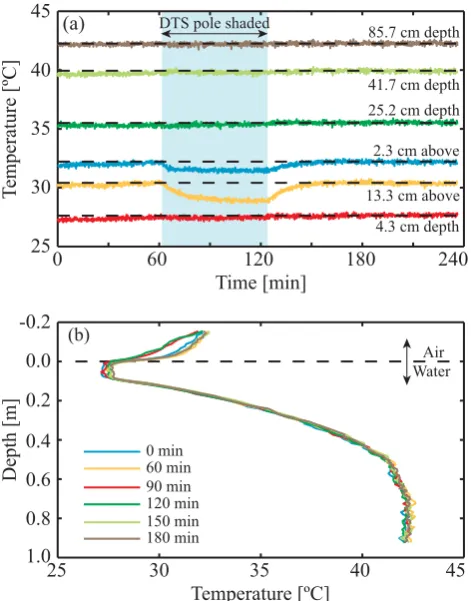
while the water temperatures below the upper convective zone were not affected when the DTS pole was shaded. As shown in Fig. 6a, after 20 min of covering the DTS pole, the temperature readings at 2.3 cm above the water level achieved a new steady-state. Here, the temperature readings were 0.7◦C lower than those without the cover. Figure 6b shows the thermal profiles measured with the DTS system
[image:10.595.98.495.62.560.2]15 20 25 30 35 -0.2
0.0
0.2
0.4
0.6
0.8
1.0
Air Water
Depth [m]
Temperature [ºC] 10-Mar-08:54
13-Mar-12:01
EC
25-Mar-12:01 17-Mar-12:02
06-Mar-08:47 DTS EC DTS
[image:11.595.51.286.62.266.2]Air Water
Fig. 5. Comparison of the temperature profile measured with the DTS system and with electrical conductivity (EC) probes. In the morning of 6 March the solar pond was filled to a depth of 0.50 m. These measurements were obtained using the manufacturer-internal calibration method.
In the upper convective zone, the temperature decreased by ∼0.1◦C when the DTS pole was shielded. When the shield was removed, the temperature of this zone increased rapidly for the first 15 min until a new steady state was reached at the end of the experiment, demonstrating how radiation absorp-tion in the DTS pole affects the temperature measurements at shallow depths.
Radiative heating of the DTS pole, for the radiation levels tested here (net radiation of 243 W m−2at the water surface – limited by the intensity of the artificial lights), was significant only when air or shallow water were measured. Temperature measurements with the DTS pole between the water surface and 10 cm depth showed only an additional 0.1◦C that was attributed to radiation absorption. Peaks of natural solar radi-ation can be 3–4 times higher than the radiradi-ation levels tested here. Hence, the impact of solar radiation absorption on the DTS pole, as well as on other temperature sensors that are not shielded, may be important when water temperatures are being measured. The systems may be especially sensitive when water velocities are very small, i.e., when conduction is the dominant heat transfer mechanism, and when the mag-nitude of solar radiation is large (Huwald et al., 2009; Neil-son et al., 2010). The impact of solar radiation absorption on fiber-optic cables can be reduced using reflective coatings or using shields to shade the cables. An optimal shield should minimize the radiation reaching the cable and the radiation absorbed by the shield, while maximizing the air or water flow around the cable (Richardson et al., 1999). If reflective coatings are used, care must be taken to not affect, i.e., warm, the surrounding environment (e.g., see Huwald et al., 2009).
Air Water DTS pole shaded
(a)
25 30 40
35 45
13.3 cm above
4.3 cm depth 25.2 cm depth 41.7 cm depth 85.7 cm depth
2.3 cm above
T
emperature [ºC]
0 60 120 180 240
Time [min]
25 30 35 40 45
-0.2
0.0
0.2
0.4
0.6
0.8
1.0
Depth [m]
0 min 60 min 90 min 120 min 150 min 180 min
(b)
Temperature [ºC]
Fig. 6. Assessment of radiative heating of the DTS pole. (a) Ther-mal evolution at different depths in the water column and in the air. (b) Temperature profile measured with the DTS system at different times of the experiment. These measurements were obtained using a 10-s integration-time interval and using the manufacturer-internal calibration method.
4 Summary and conclusions
As temperature is a major driver of changes in natural and managed aquatic systems, there is a need to observe temper-atures at high spatial and temporal resolutions. The verti-cal high-resolution DTS system provides a reliable method to monitor temperature in space and time, which is essen-tial in many hydrological applications such as thermohaline environments. In addition, the presented DTS system over-comes the problems typical of methods used in the past such as drift due to corrosive environment. This is a major issue in thermohaline systems, particularly in solar ponds where the salinity approaches saturation.
[image:11.595.310.546.63.364.2]in time averages as small as 10 s. Temperature resolution as low as 0.035◦C was obtained when the data were collected
at 5 min intervals. It was found that the DTS system resolved temperatures with very small variability using either single-or double-ended measurements, and that the observed noise in the system could be due to a combination of white and flicker noise. Using the vertical high-resolution DTS system, stratification, mixing, interface erosion, and freshwater re-supply were observed in the solar pond at a resolution that is hardly achievable using traditional temperature sensors. In our experimental setup, radiation absorption was found to be significant only when air or shallow water temperatures were measured. However, it may be important in systems exposed to natural solar radiation.
Acknowledgements. The authors wish to thank the Department of Energy (DOE) for funding Grants DE-FG02-05ER64143 and 656-1769-01-NV-REC (Nevada Renewable Energy Consortium), and the National Science Foundation (NSF) for partial funding of this work by Award NSF-EAR-0929638. The authors greatly appreciate the support of Jeffrey Ruskowitz, the valuable input from John S. Selker, and the constructive suggestions of Mar-tijn Westhoff, Hendrik Huwald (reviewers) and Ty Ferre (editor).
Edited by: T. P. A. Ferre
References
Anati, D. A. and Stiller, M.: The post-1979 thermohaline structure of the dead-sea and the role of double-diffusive mixing, Limnol. Oceanogr., 36, 342–354, 1991.
Bejan, A.: Convection Heat Transfer, 3rd edition, John Wiley and Sons, Inc, New Jersey, 2004.
Bergman, T. L., Incropera, F. P., and Stevenson, W. H.: Miniature fiber-optic refractometer for measurement of salinity in double-diffusive thermohaline systems, Rev. Sci. Instrum., 56, 291–296, 1985.
Box, G., Jenkins, G., and Reinsel, G.: Time Series Analysis. Fore-casting and Control, 4th edition, John Wiley and Sons, Inc, New Jersey, 2008.
Branco, B., Torgersen, T., Bean, J. R., Grenier, G., and Arbige, D.: A new water column profiler for shallow aquatic systems, Lim-nol. Oceanogr. Meth., 3, 190–202, 2005.
Branco, B. F. and Torgersen, T.: Predicting the onset of thermal stratification in shallow inland waterbodies, Aquat. Sci., 71, 65– 79, 2009.
Dakin, J. P., Pratt, D. J., Bibby, G. W., and Ross, J. N.: Distributed optical fiber Raman temperature sensor using a semiconductor light-source and detector, Electron. Lett., 21, 569–570, 1985. Farahani, M. A. and Gogolla, T.: Spontaneous Raman scattering in
optical fibers with modulated probe light for distributed temper-ature Raman remote sensing, J. Lightwave Technol., 17, 1379– 1391, 1999.
Huwald, H., Higgins, C. W., Boldi, M. O., Bou-Zeid, E., Lehn-ing, M., and Parlange, M. B.: Albedo effect on radiative errors in air temperature measurements, Water Resour. Res., 45, W08431, doi:10.1029/2008WR007600, 2009.
Kaulakys, B. and Alaburda, M.: Modeling scaled processes and 1/fβ noise using nonlinear stochastic differential equa-tions, J. Stat. Mech.-Theory E., P02051, doi:10.1088/1742-5468/2009/02/P02051, 2009.
Kersey, A. D.: Optical fiber sensors for permanent downwell moni-toring applications in the oil and gas industry, IEICE T. Electron., E83-C, 400–404, 2000.
Kurt, H. and Ozkaymak, M.: Performance evaluation of a small-scale sodium carbonate salt gradient solar pond, Int. J. Energ. Res., 30, 905–914, 2006.
Lawrence, A., Watson, M. G., Pounds, K. A., and Elvis, M.: Low-frequency divergent X-ray variability in the Seyfert galaxy NGC4051, Nature, 325, 694–696, 1987.
Lorke, A., Tietze, K., Halbwachs, M., and Wuest, A.: Response of Lake Kivu stratification to lava inflow and climate warming, Limnol. Oceanogr., 49, 778–783, 2004.
Losordo, T. M. and Piedrahita, R. H.: Modeling temperature vari-ation and thermal stratificvari-ation in shallow aquaculture ponds, Ecol. Model., 54, 189–226, 1991.
Lu, H. M., Swift, A. H. P., Hein, H. D., and Walton, J. C.: Ad-vancements in salinity gradient solar-pond technology based on sixteen years of operational experience, J. Sol. Energ.-T. ASME, 126, 759–767, 2004.
McDowell, E. J., Ren, J., and Yang, C.: Fundamental sensitivity limit imposed by dark 1/f noise in the low optical signal detec-tion regime, Opt. Express, 16, 6822–6832, 2008.
Moffett, K. B., Tyler, S. W., Torgersen, T., Menon, M., Selker, J. S., and Gorelick, S. M.: Processes controlling the thermal regime of saltmarsh channel beds, Environ. Sci. Technol., 42, 671–676, 2008.
Neilson, B. T., Hatch, C. E., Ban, H., and Tyler, S. W.: Solar radiative heating of fiber-optic cables used to moni-tor temperatures in water, Water Resour. Res., 46, W08540, doi:10.1029/2009WR008354, 2010.
Richardson, S. J., Brock, F. V., Semmer, S. R., and Jirak, C.: Mini-mizing errors associated with multiplate radiation shields, J. At-mos. Ocean. Tech., 16, 1862–1872, 1999.
Rogers, A.: Distributed optical-fibre sensing, Meas. Sci. Technol., 10, R75–R99, 1999.
Rosenzweig, C., Casassa, G., Karoly, D. J., Imeson, A., Liu, C., Menzel, A., Rawlins, S., Root, T. L., Seguin, B., and Try-janowski, P.: Assessment of observed changes and responses in natural and managed systems, in: Climate Change 2007: Impacts, Adaptation and Vulnerability. Contribution of Work-ing Group II to the Fourth Assessment Report of the Intergov-ernmental Panel on Climate Change, edited by: Parry, M. L., Canziani, O. F., Palutikof, J. P., and van der Linden, P. J., Cam-bridge University Press, 79–131, 2007.
Rubiola, E.: On the measurement of frequency and of its sample variance with high-resolution counters, Rev. Sci. Instrum., 76, 054703, doi:10.1063/1.1898203, 2005.
Selker, J. S., Thevenaz, L., Huwald, H., Mallet, A., Luxemburg, W., van de Giesen, N. C., Stejskal, M., Zeman, J., Westhoff, M., and Parlange, M. B.: Distributed fiber-optic temperature sens-ing for hydrologic systems, Water Resour. Res., 42, W12202, doi:10.1029/2006WR005326, 2006.
Su´arez, F., Tyler, S. W., and Childress, A. E.: A theoretical study of a direct contact membrane distillation system coupled to a salt-gradient solar pond for terminal lakes reclamation, Water Res., 44, 4601–4615, 2010b.
Su´arez, F., Childress, A. E., and Tyler, S. W.: Temperature evolu-tion of an experimental salt-gradient solar pond, J. Water Climate Change, 1, 246–250, 2010c.
Tyler, S. W., Burak, S. A., Mcnamara, J. P., Lamontagne, A., Selker, J. S., and Dozier, J.: Spatially distributed temperatures at the base of two mountain snowpacks measured with fiber-optic sensors, J. Glaciol., 54, 673–679, 2008.
Tyler, S. W., Selker, J. S., Hausner, M. B., Hatch, C. E., Torgersen, T., Thodal, C. E., and Schladow, S. G.: En-vironmental temperature sensing using Raman spectra DTS fiber-optic methods, Water Resour. Res., 45, W00D23, doi:10.1029/2008WR007052, 2009.
Vogt, T., Schneider, P., Hahn-Woernle, L., and Cirpka, O. A.: Es-timation of seepage rates in a losing stream by means of fiber-optic high-resolution vertical temperature profiling, J. Hydrol., 380, 154–164, 2010.
Westhoff, M. C., Savenije, H. H. G., Luxemburg, W. M. J., Stelling, G. S., van de Giesen, N. C., Selker, J. S., Pfister, L., and Uh-lenbrook, S.: A distributed stream temperature model using high resolution temperature observations, Hydrol. Earth Syst. Sci., 11, 1469–1480, doi:10.5194/hess-11-1469-2007, 2007.