https://doi.org/10.5194/hess-21-6541-2017 © Author(s) 2017. This work is distributed under the Creative Commons Attribution 3.0 License.
Development and evaluation of a stochastic daily rainfall model
with long-term variability
A. F. M. Kamal Chowdhury1,a, Natalie Lockart1, Garry Willgoose1, George Kuczera1, Anthony S. Kiem2, and Nadeeka Parana Manage1
1School of Engineering, The University of Newcastle, Callaghan 2308, New South Wales, Australia 2School of Environmental and Life Sciences, The University of Newcastle, Callaghan 2308, New South Wales, Australia
anow at: Department of Civil Engineering, International University of Business Agriculture and Technology, Dhaka 1230, Bangladesh
Correspondence:Garry Willgoose ([email protected]) Received: 14 February 2017 – Discussion started: 27 February 2017
Revised: 7 July 2017 – Accepted: 9 October 2017 – Published: 22 December 2017
Abstract.The primary objective of this study is to develop a stochastic rainfall generation model that can match not only the short resolution (daily) variability but also the longer res-olution (monthly to multiyear) variability of observed rain-fall. This study has developed a Markov chain (MC) model, which uses a two-state MC process with two parameters (wet-to-wet and dry-to-dry transition probabilities) to sim-ulate rainfall occurrence and a gamma distribution with two parameters (mean and standard deviation of wet day rain-fall) to simulate wet day rainfall depths. Starting with the traditional MC-gamma model with deterministic parameters, this study has developed and assessed four other variants of the MC-gamma model with different parameterisations. The key finding is that if the parameters of the gamma distribu-tion are randomly sampled each year from fitted distribudistribu-tions rather than fixed parameters with time, the variability of rain-fall depths at both short and longer temporal resolutions can be preserved, while the variability of wet periods (i.e. num-ber of wet days and mean length of wet spell) can be pre-served by decadally varied MC parameters. This is a straight-forward enhancement to the traditional simplest MC model and is both objective and parsimonious.
1 Introduction
Observed rainfall data generally provide a single realisation of a short record, often not more than a few decades. The direct application of these data in hydrological and agricul-tural systems may not provide the necessary robustness in identification and implication of extreme climate conditions (e.g. droughts, floods). In particular, for urban water secu-rity analysis of reservoirs, long-term hydrologic records are required to sample extreme droughts that drive the security of the urban system (Mortazavi et al., 2013). However, the observed data may still be suitable to calibrate stochastic rainfall models that can, in turn, be used to generate long stochastic streamflow sequences for use in reservoir reliabil-ity modelling. In addition to historical and current scenarios, the stochastic models are useful to evaluate the climate and hydrological characteristics of future climate change scenar-ios (Glenis et al., 2015).
variability of rainfall may cause an overestimation of reser-voir reliability in urban water planning (Frost et al., 2007). Therefore, preserving key statistics of wet and dry spells, and rainfall depths in daily to multiyear resolutions, is important in stochastic rainfall simulation.
Markov chain (MC) models are very common for stochas-tic rainfall generation. A typical MC rainfall model is com-posed of two parts: a rainfall occurrence model that uses a transition probability between wet and dry days, and a rain-fall magnitude model that uses a probability distribution of wet day rainfall depths (commonly a gamma distribution) fitted to the observed data. The two-part MC-gamma model is one of the most popular parametric models for daily rain-fall simulation, primarily proposed by Richardson (1981) and known as WGEN (weather generator). In addition to rainfall, the WGEN also simulates temperature and solar radiation. While other models such as point process models (Cowpert-wait et al., 1996) are also used for stochastic rainfall genera-tion, this study has focused on MC-type models.
The first component of the MC model defines wet and dry days. This is determined by the state and order of the Markov process. Most MC models (Richardson, 1981; Dubrovský et al., 2004) use a simple two-state, first-order approach, that is, a day can be either “wet” or “dry” (two-state) and the state of the current day is only dependent on the state of the preced-ing day (first-order). Other models use higher states and or-ders; examples include the four-state model (Jothityangkoon et al., 2000), the alternating renewal process model with negative binomial distribution of wet and dry spell lengths (Wilby et al., 1998), the bivariate mixed distribution model (Li et al., 2013), and the multi-order model (Lennartsson et al., 2008). These models are more complex as the num-ber of parameters required in the model increases with the number of states and orders of the Markov process. How-ever, the two-state, first-order MC model can often repro-duce the statistics of wet and dry periods just as well as these higher state/order models (Chen and Brissette, 2014). Dubrovský et al. (2004) recommended that, rather than try-ing an increased order MC, one should consider other ap-proaches for better reproduction of wet and dry days. Mehro-tra and Sharma (2007) proposed a modified MC process us-ing memory of past wet periods, which has been found to reproduce the wet and dry spell statistics reasonably well. They also tested a first-order and a second-order process in their modified MC model and found that the second-order process provided only marginal improvements over the first-order process. Another important finding of Dubrovský et al. (2004) was that the order of MCs generally had no effect on the variability of monthly rainfall depths.
The second component of the MC model is the prob-ability distribution for the wet day rainfall. As the distri-bution of wet day rainfall is generally right-skewed (Hun-decha et al., 2009), it is common practice to use right-skewed exponential-type distributions. Common distribu-tions include the gamma distribution (Wang and Nathan,
2007; Chen et al., 2010), Weibull distribution (Sharda and Das, 2005), truncated normal distribution (Hundecha et al., 2009), and kernel-density estimation techniques (Harrold et al., 2003). A number of other studies fitted a mixture of two or more distributions; for example, the mixed expo-nential distribution (Wilks, 1999a; Liu et al., 2011), gamma and generalised Pareto distribution (Furrer and Katz, 2008), and transformed normal and generalised Pareto distribution (Lennartsson et al., 2008). However, the gamma distribution is the most commonly used distribution, because it has only two parameters, that can be calculated from the mean and standard deviation (SD) of wet day rainfall, and adequately represent the rainfall probability distribution functions. The parameterisation and application of the distribution in the model is straightforward. Although the gamma distribution has been found to be appropriate for simulating most of the variability in rainfall depth (Bellone et al., 2000), the major drawback of using a gamma distribution is that its tail is too light to capture heavy rainfall intensities (Vrac and Naveau, 2007). Therefore, direct use of a gamma distribution usually causes an underestimation of SD and extreme rainfall depths at monthly to multiyear resolutions.
A number of methods have been developed in an attempt to resolve the underestimation of long-term variability. The major approaches for resolving this issue include (i) models with mixed distributions, (ii) nesting-type models, (iii) mod-els with rainfall-climate index correlation, and (iv) modmod-els with modified Markov chains.
Nesting models adjust the daily rainfall series at differ-ent temporal resolutions to obtain statistics that are optimal for all resolutions. These models initially generate a daily rainfall series, which is then modified to adjust the monthly and yearly statistics. Several models (Dubrovský et al., 2004; Wang and Nathan, 2007; Srikanthan and Pegram, 2009; Chen et al., 2010) use the nesting method. They generally generate a daily rainfall series, then the generated daily rainfall data are aggregated to monthly rainfall values, and these monthly values are modified by a lag–1 autoregressive monthly rain-fall model. The modified monthly rainrain-fall values are aggre-gated to annual rainfall values and these values are then mod-ified by another lag–1 autoregressive annual model (Srikan-than and Pegram, 2009). The nesting-type models gener-ally perform well to reproduce the rainfall variability at all resolutions. Dubrovský et al. (2004) also showed satisfac-tory performance of their nesting-type model to reproduce the variability of monthly streamflow characteristics and the frequency of extreme streamflow. Although the nesting-type models preserve the daily, monthly and yearly statistics, they are generally based on subjective statistical adjustments and thus have a weak physical basis.
Some parametric models introduced the influence of large-scale climate mechanisms such as the El Niño/Southern Os-cillation (ENSO) in parameterisation (Hansen and Mavroma-tis, 2001; Furrer and Katz, 2007). Bardossy and Plate (1992) used the correlation between atmospheric circulation pat-terns and rainfall in a transformed conditional multivariate autoregressive AR(1) model for daily rainfall simulation. Katz and Parlange (1993) developed a model with parame-ters conditioned on the ENSO indices. Yunus et al. (2016) developed a generalised linear model for daily rainfall by us-ing ENSO indices as predictors. Although the climate indices were often not strongly correlated to the rainfall, Katz and Zheng (1999) described it as a diagnostic element to detect a “hidden” (i.e. unobserved) index, which could be used to ob-tain long-term variability. Thyer and Kuczera (2000) devel-oped a hidden state MC model for annual data, while Ramesh and Onof (2014) developed a hidden state MC model for daily data. The major drawback of this model approach is that the hidden index is unobserved and its origin is un-known.
Modified MC models concentrate not only on the order of MC but also introduce modifications to the parameterisation of the MC process to better reproduce the rainfall variability. The transition probabilities are generally modified by consid-ering their long-term variability (i.e. memory of past wet and dry periods), and the wet day rainfall depth is modelled using a nonparametric kernel-density simulator conditional on pre-vious day rainfall (Lall et al., 1996; Harrold et al., 2003). The nonparametric kernel-density techniques usually used resampling of observed data (Rajagopalan and Lall, 1999). While these models perform reasonably well, they usually cannot generate extreme values higher than the observed ex-tremes, because only the original observations are
resam-pled in the model (Sharif and Burn, 2006). Mehrotra and Sharma (2007) proposed a semi-parametric Markov model, which was further evaluated by Mehrotra et al. (2015). To in-corporate the long-term variability, they modified the transi-tion probabilities of the MC process by taking the memory of past wet periods (i.e. beyond lag–1) into account, while the wet day rainfall depths were simulated by a nonparametric kernel-density process. For rain gauge data around Sydney, the semi-parametric model preserved the rainfall variability at daily to multiyear resolutions (Mehrotra et al., 2015).
The MC models that focus specifically on resolving the underestimation of long-term variability involve subjective assumptions and limitations. In the models with mixed distri-butions, defining a certain rainfall depth as an extreme value is subjective. The nesting-type models used empirical adjust-ment factors, generally without physical foundation. The hid-den indices of hidhid-den state MC models are unobserved. The models with modified MC parameters, modified the transi-tion probabilities of wet and dry periods to obtain long-term variability, but used the kernel-density technique to resam-ple wet day rainfall depths from observed records. Therefore, they usually cannot generate more extreme values than the observed extremes.
The overarching objective of the research, that this paper forms part of, is to develop a stochastic rainfall generator that can be calibrated to daily rainfall data derived from dynami-cally downscaled global climate simulations, and which also preserves long-term variability (Evans et al., 2014). A com-mon problem with these simulations is that typical compu-tational CPU limits mean that the length of the simulation is rarely more than a few decades, not long enough to facili-tate stochastic assessment of the reliability of water supply reservoirs (e.g. Lockart et al., 2016). Accordingly, we need a rainfall simulator that can be calibrated and run at the daily timescale (to be used as input into a hydrology model at the daily resolution), but which has the right statistical properties (specifically variability about the mean) when averaged over periods up to a decade. In this paper, we develop and test five models using observed rainfall at two sites in Australia with contrasting climates.
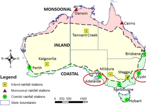
per-Figure 1.Location map of 12 rain gauge stations around Australia. This study has presented the assessment results of the developed models for Sydney and Adelaide stations (red circled) only. The shaded green, yellow, and red colours indicate the coastal, inland, and monsoonal areas, respectively.
formance against the incremental increases in model com-plexity.
2 Data and study sites
This study has used daily rain gauge data from Sydney Ob-servatory Hill and Adelaide Airport stations (station num-ber 66062 and 023034, respectively) obtained from the Bu-reau of Meteorology (BoM), Australia (Fig. 1) for 1979– 2008 (BoM, 2013). These two stations have been used be-cause they provide a contrast between a highly seasonal Mediterranean climate with low interdecadal variability in Adelaide and a relatively non-seasonal climate with high interdecadal variability in Sydney (see Fig. 2). Risbey et al. (2009) also showed that the major climate drivers of rain-fall (e.g. ENSO) in Sydney and Adelaide are different for all seasons. This paper also used the Oceanic Nino Index (ONI) and the Interdecadal Pacific Oscillation (IPO) index at monthly resolution for the 1979–2008 period (Folland, 2008; NOAA, 2014). These climate indices are used to develop two variants of the MC models discussed in Sect. 4.2.2.
3 Model assessment procedures
3.1 Statistics for assessment of model performance Each model developed in this study has been assessed to un-derstand its ability to reproduce the distribution and autocor-relation of observed rainfall. Assessment of the distribution and autocorrelation are generally used to inform the suitabil-ity of the model for urban drought secursuitabil-ity assessment. The assessment criteria of each model consider its ability to
re-produce (i) mean, SD, and 95th percentile of rainfall depths at daily to multiyear resolutions; (ii) mean and SD of the number of wet days and mean length of wet spells at monthly to multiyear resolutions; and (iii) month-to-month autocor-relations of monthly rainfall depths and monthly number of wet days. The performances of the MC models for dry pe-riod statistics are found to be similar to the wet pepe-riod statis-tics (the term “wet period statisstatis-tics” will hereafter refer to the number of wet days and mean length of wet spells), and hence, only representative results for annual mean length of dry spells are shown.
At daily and monthly resolutions, the distribution statistics are assessed for each month starting from January; while at multiyear resolutions, the distribution statistics are assessed for 1 to 10 overlapping years. Mean length (in days) of wet spells are calculated at monthly, and annual resolution by ex-tracting wet spells of one or more consecutive wet days (two successive wet spells are separated by at-least one dry day) and using Eq. (1):
mean length of wet spell= P
(length of wet spells)
P
(occurrences of wet spells). (1)
Similar to wet spells, the mean length of dry spells are also calculated at monthly and annual resolution by extracting dry spells of one or more consecutive dry days.
3.2 Calculation ofZscores
For the distribution statistics (i.e. mean and SD) of rainfall depths and wet periods (number of wet days and mean length of wet spells), this study has calculated the expected value and error limit (SD) to calculate theZscore of a model sim-ulation. The calculation of theZscore is as follows:
1. Run the model 1000 times using the probability distri-bution of the parameters calibrated to the observed data, with each run being the same length as the observed data.
2. Calculate the desired statistics (e.g. mean and SD of the daily rainfall depths) in each run, which gives 1000 re-alisations of each statistic.
3. For each statistic, calculate the mean (expected value) and SD (error limit) of the 1000 realisations.
4. Calculate theZscore of each statistic by comparing the expected value with the respective observed value (cal-culated from the observed data), as follows:
ZScore=Observed value−Expected value
SD . (2)
[image:4.612.48.286.69.242.2]of the simulated rainfall, assuming a normal distribution ap-proximates the sampling distribution of Z. A Z score less than−2 or greater than+2 suggests that the statistic is over-or under-estimated, respectively, in the model simulation.
4 Markov chain (MC) models
This study has developed and assessed the following five variants of a Markov chain (MC) model:
– Model 1: Average Parameter Markov Chain (APMC) model,
– Model 2: Decadal Parameter Markov Chain (DPMC) model,
– Model 3: Compound Distribution Markov Chain (CDMC) model,
– Model 4: Hierarchical Markov Chain (HMC) model, – Model 5: Decadal and Hierarchical Markov Chain
(DHMC) model.
4.1 Model 1: Average Parameter Markov Chain (APMC) model
The first MC model – the APMC – is a traditional two-part MC-gamma distribution model. This is similar to the rainfall generator proposed by Richardson (1981), widely known as the WGEN model. The exception is that the parameters in WGEN were smoothed with Fourier harmonics, which has not been done in the case of APMC parameters. Although APMC is not the final model of this study, it is the base-line modelling approach against which the more sophisti-cated models developed in this study are compared.
The APMC simulates the daily rainfall in two steps: daily rainfall occurrence (i.e. wet and dry day) simulation by first-order Markov chain, and wet day rainfall depth simulation by gamma distribution. To incorporate the seasonal variability in the model, the APMC uses a separate set of parameters for each month, where the first month of the simulation is January.
4.1.1 Rainfall occurrence simulation
The APMC uses 24 (2 parameters×12 months) MC param-eters, and transition probabilities of dry-to-dry day (P00)and wet-to-wet day (P11)for dry and wet day occurrence simu-lation. In addition, the unconditional probability of a dry day (π0)in January is used to simulate rainfall occurrence for the first day of the series. In the model calibration, these de-terministic MC parameters are calculated from the observed daily rainfall data. To calculate these parameters, a day with rainfall depth of 0.3 mm and above has been considered a wet day, otherwise it was considered a dry day (similar to Mehro-tra et al., 2015). In simulation, the MC parameters are used
in a Monte-Carlo process to simulate the occurrences of wet and dry days.
4.1.2 Rainfall depth simulation
After simulation of the rainfall occurrence using MC param-eters, the next step is to generate rainfall depths for the wet days. The rainfall depth for dry days is zero. The APMC rain-fall depth simulation process assumes that (i) daily rainrain-fall depth for wet days follows a gamma distribution, and (ii) the rainfall depth for a wet day is independent of the rainfall depth of the preceding day.
The gamma distribution has two parameters,α(shape pa-rameter) and β (scale parameter), with mean µ=αβ and variance σ2=αβ2. Since both αi andβi are directly pro-portional to and can be derived fromµi andσi of wet day rainfall of the monthi, then during calibration of the model it is convenient to calculateµi andσi values from the daily rainfall observed data. The appropriate ratios ofµiandσican then be used in the rainfall depth generation process using the gamma distribution. Therefore,µi andσi will be referred to as the gamma distribution parameters in further discussions of this paper.
In the calibration of APMC, deterministic average values ofµi andσi are calculated from the entire period of the data record for each month. This gives 12 values ofµandσeach. In simulations, the rainfall depth for each wet day of a month
i is generated using theµi andσi values of the respective month using the gamma distribution. In generating the rain-fall depth for a wet day, if a random sample from the gamma distribution gives a rainfall depth less than 0.3 mm then the rainfall for that day is set to 0.3 mm (i.e. the threshold rain-fall depth), while the rainrain-fall depths for dry days are set to 0.0 mm. Chowdhury (2017) showed that setting rainfall be-low 0.3 mm to 0.3 mm for the be-lowest rainfall depth does not significantly affect the overall distribution of modelled rain-fall depths.
4.1.3 Independence of rainfall depths in successive wet days
The APMC assumes that the rainfall depth for a particular day is independent of the rainfall depth of the preceding day. To validate this assumption, this study examined the auto-correlation of wet day rainfall depths, and only found very weak lag–1 autocorrelations (r2< 0.1) for both Sydney and Adelaide. This finding is consistent irrespective of seasonal variations. The conclusion is that the underlying assumption of daily independence of the APMC is consistent with the respective characteristic of the observed data.
4.2 Model 2: Decadal Parameter Markov Chain (DPMC) model
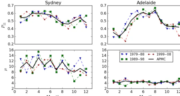
res-Figure 2.Comparison of the decadal variability of the DPMC parametersP11andµ(mm) with the APMC parameters.
olutions. The DPMC assumes that the interannual rainfall variability can be captured by the decade-to-decade variabil-ity of the parameters that APMC failed to capture. The idea is to divide the observed rainfall sample into subsamples of 10 years duration (similar models with climate-based sub-samples are discussed in Sect. 4.2.2). For example, a 30-year rainfall sample is divided into three subsamples of 10 years in duration. Then, 4×12 parameters ofP00,P11,µ, andσ(one set of four parameters for each of the 12 months) are calcu-lated from each of the subsamples. The simulation proceeds in a way similar to the APMC, except that the determinis-tic, decadal average, parameters of DPMC are varied from decade to decade.
4.2.1 Decadal variability of DPMC parameters
Figure 2 shows the DPMC values of P11 and µ for each decade along with APMC values (i.e. the 30-year averages) for Sydney and Adelaide. For Sydney, DPMC values ofP11 andµshow clear variability between the three decadal sam-ples and deviations from the APMC values. However, DPMC values ofP11 andµfor Adelaide show less variability be-tween the decadal samples.
The use of decadally varied parameters in DPMC is sub-ject to the question of how significant the decadal variability of these parameters is – is the decadal variability statistically significant or just sampling variability? Therefore, the sta-tistical significance of the decadal variability of DPMC pa-rameters were examined by Monte-Carlo simulations as per Sect. 3.2. This examination suggested that the sampling vari-ability of DPMC parameters in decadal samples is mostly within the sampling variability of their corresponding APMC values (not shown). This suggests that the decadal variability of DPMC parameters is not statistically significant.
4.2.2 Potential impact of climate modes
This study has also investigated other subsampling ap-proaches of the MC-gamma parameters similar to the DPMC. In these models, this study has calibrated the MC-gamma parameters to subsamples of rainfall time series di-vided according to the phases of IPO (e.g. positive and neg-ative) and ENSO (La Niña, Neutral, and El Niño). Since previous studies (Verdon-Kidd et al., 2004) found that the interannual variabilities of east-Australian rainfall are influ-enced by these large-scale climate drivers, the idea behind these models was to introduce more interannual variability to the model by simulating rainfall for different phases of cli-mate drivers with parameters calibrated to respective phases. These climate-based models are very similar to DPMC, ex-cept that the subsamples are different. The following two types of climate-based models have been tested:
– The IPO based model: the observed data for every month was divided into two subsamples according to the positive and negative phases of the monthly IPO in-dex (e.g. for January, data of the years with positive IPO index and data of the years with negative IPO index are separated). Then, for each month, the MC-gamma parameters (P00,P11,µ, andσ ) are calibrated to each subsample. In simulation, the rainfall for the months of each IPO phase were modelled by using parameters of the respective phase.
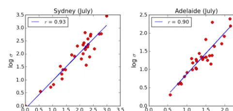
[image:6.612.143.457.67.235.2]Figure 3.Lognormal probability plots ofµandσfor July (typical of other months).
4.3 Model 3: Compound Distribution Markov Chain (CDMC) model
The results in Sect. 6 will show that neither APMC nor DPMC can satisfactorily reproduce the SD of rainfall depths for monthly to multiyear resolutions. Therefore, in the third MC model – the CDMC – this study has incorporated the long-term variability of rainfall depths by introducing ran-dom variability inµandσ. However, for wet and dry period simulation, the CDMC still uses the deterministic parameters ofP00andP11, as in the APMC. Thus, this model stochasti-cally varies the rainfall depth model, but not the rainfall oc-currence model.
In the CDMC,µi andσi are randomly sampled for each month of each year. The random sampling was done inde-pendently of the sampling for the preceding month(s). To es-timate the distribution ofµi andσi, this study has calculated
µi andσi for every month of every year from the observed data. For example, from the 30-year observed data, for Jan-uary (i=1), this study has calculated 30 samples ofµ1and
σ1values each.
By testing the probability distributions ofµi andσi val-ues for each month, this study has found that bothµiandσi values for each month are lognormally distributed. Figure 3 shows the lognormal probability plots ofµiandσivalues for July (i=7), which is representative of the other months. The
r2for logµi and logσi are generally above 0.90, indicating a very good fit of the lognormal distributions. Additionally, the hypothesis that logµiand logσiare normally distributed is supported by the Kolmogorov–Smirnov test at 5 % signifi-cance level. In addition to the lognormally distributedµiand
σi values, this study has also found that the logµiand logσi values for each month are strongly correlated with each other with correlation coefficientrc,i around 0.90 (Fig. 4). There-fore, for each monthi, this study has fitted a bivariate-normal distribution to the logµi and logσi values with parameters (λµ,i,ζµ,i), (λσ,i,ζσ,i), andrc,i. Theλandζ parameters de-note the mean and SD of the log variate, whilercis the cor-relation coefficient between logµand logσ.
At the start of each month of each year of the simulation, the logµi is sampled from its fitted normal distribution log
Figure 4.Correlation between logµand logσfor July (typical of other months).
µi∼N (λµiζ
2
µi) for month i. Then, the log σi is sampled
from the fitted conditional normal distribution: logσi|logµi
∼N
λσi+
ζσi
ζµi
rc,i logµi−λµi
1−rc2,i
ζσi
2
. (3)
These stochastically sampledµi andσi values are then used to generate rainfall in the wet days for the month in question, while the sequence of wet and dry days is determined using the deterministic APMC values ofP00,i andP11,i. However, the sampledµiandσivalues of a month (i)are not correlated to theµi−1andσi−1of the preceding month (i−1) as this study has found that the month-to-month autocorrelations of
µandσ values are not strong (Fig. 5).
4.4 Model 4: Hierarchical Markov Chain (HMC) model
[image:7.612.308.549.230.344.2]Figure 5.Month-to-month autocorrelations ofP00,P11,µ, andσ
for(a)Adelaide and(b)Sydney. The shadings indicate 95 % confi-dence limits.
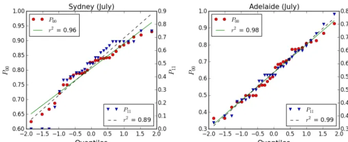
i, theseP00,i andP11,i values (e.g. 30P11,7values for July from the 30-year observed data) are found to be normally dis-tributed with values between 0 and 1 (Fig. 6). Therefore, this study has fitted a truncated normal distribution, bounded by 0 and 1, to the calculatedP00 andP11values. In simulation, for each year, theP00,iandP11,iare sampled from their trun-cated normal distributions. This procedure is similar to what was done forµi andσi to sample from bivariate-lognormal distribution. However, it does not include a bivariate distri-bution because the correlation betweenP00,i andP11,i was weak.
4.4.1 Impact of autocorrelations on stochasticity of MC parameters
In the HMC, the sampled MC parameters of each month are independent of the parameters of the preceding month.
How-ever, this study has found strong month-to-month autocorre-lations of theP00 andP11 for Adelaide (Fig. 5a), although the autocorrelations are weak for Sydney (Fig. 5b). There-fore, this study has tested an alternative to the HMC (referred to as HMC2), which uses a lag–1 autocorrelation equation (a similar equation was used by Wang and Nathan (2007) in their rainfall depth model) in the stochastic sampling ofP00,i andP11,ifrom the truncated normal distribution. The follow-ing lag–1 autocorrelation equation has been used to modify the randomly sampledP00,i (same method used forP11,i) for monthiby correlating with theP00,i−1 of monthi−1 (preceding month):
P00,i−mean(P00,i) sd(P00,i)
=r×P00,i−1−mean(P00,i−1)
sd(P00,i−1)
+(1−r2)1/2P00,i−mean(P00,i)
sd(P00,i)
, (4)
where for a monthi(e.g. January),
– mean(P00,i)is the mean of the yearly varied parameter values calculated from observed data for monthi (e.g. mean of 30P00,7values for July),
– sd(P00,i)is the SD of the yearly varied parameter values calculated from observed data for monthi,
– mean(P00,i−1)is the mean of the parameter values cal-culated from observed data for monthi−1,
– sd(P00,i−1)is the SD of the parameter values calculated from observed data for monthi−1,
– r is the lag–1 autocorrelation coefficient for observed month-to-month autocorrelation ofP00(constant for all month),
– P00,i is the stochastic parameter value sampled from a truncated normal distribution fitted to the yearly varied observed parameter values for monthi,
– P00,i−1 is auto-correlated parameter value for month
i−1 (used to simulate the dry days of the preceding month),
– P00,i is the final auto-correlated parameter value which was used in simulation of dry days for monthi.
P11,i for monthiis sampled using a similar process. 4.4.2 Impact of cross-correlations on stochasticity of
MC parameters
Figure 6.Normal probability plots ofP00andP11for July (typical of other months).
and logµi and logσi are weak. Therefore, another alterna-tive to HMC (referred to as HMC3) was tested by using a multivariate sampling system for theP11,i,µi, andσi, while
P00,i remains independent.
4.5 Model 5: Decadal and Hierarchical Markov Chain (DHMC) model
Section 6 will show that the CDMC, with APMC values of MC parameters, significantly underestimates the wet period variability at multiyear resolutions, while the HMC (includ-ing the two alternatives HMC2 and HMC3) with stochastic MC parameters, significantly overestimates the wet period variability at monthly resolution. However, we found that the DPMC can satisfactorily preserve the wet period vari-ability at both monthly and multiyear resolutions, although it underestimates the rainfall depth variability. Therefore, in the DHMC model, this study has used the DPMC values of MC parameters (the parameter values vary for each decade of simulation) for simulation of wet and dry days, while the stochastic parameters of the gamma distribution (same as CDMC) are used for simulation of wet day rainfall depths.
5 Methodological comparison of five MC models
The following points discuss the key common features in the five MC models of this study, while other key methodological comparisons are shown in Table 1:
– All models use first-order MC parameters to simulate the rainfall occurrences and gamma distribution to sim-ulate rainfall depths in wet days.
– Simulation of rainfall depth for each wet day is inde-pendent of the rainfall depth of the preceding day. – Separate sets of parameters are used for each month
(e.g. 12 sets of MC and gamma parameters) to incor-porate seasonal variability.
6 Model comparison for distribution statistics
This section compares the performances of the five MC mod-els for the mean and SD of rainfall depths and wet period statistics (i.e. number of wet days and mean length of wet spells).
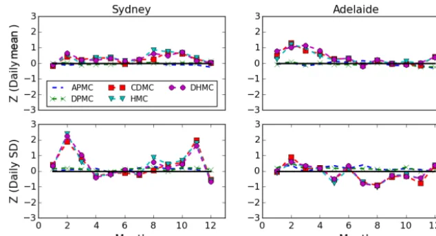
6.1 Mean and SD of rainfall depths
Figures 7, 8, and 9 compare the five MC models for the mean and SD of rainfall depths at daily, monthly, and mul-tiyear resolutions, respectively. Figure 9 also compares the 95th percentile of multiyear rainfall depths. For mean and SD of rainfall depths, the performances of APMC and DPMC are similar. The performances of CDMC, HMC, and DHMC are also similar, but different from APMC and DPMC. All five models preserve the mean (i.e. satisfactorily reproduce the observed mean) rainfall depths at all resolutions with
Table 1.Methodological comparison of the five MC models.
Wet and dry day simulation Wet day rainfall depth simulation
APMC Uses deterministic MC parameters, same set of parameters for each simulation year.
Uses deterministic gamma parameters, same set of parameters for each simulation year.
DPMC Uses decadally varied deterministic MC parame-ters.
Uses decadally varied deterministic gamma parameters.
CDMC Same as APMC. Uses stochastic parameters (sampled from fitted
bivariate-lognormal distribution) of gamma distribu-tion, parameters vary for each simulation year.
HMC Uses stochastic MC parameters (sampled from fit-ted truncafit-ted normal distribution), parameters vary for each simulation year.
Same as CDMC.
DHMC Same as DPMC. Same as CDMC.
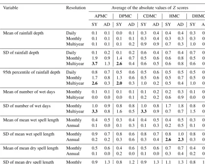
Table 2.Average of the absolute values ofZscores (average of theZscores for all 12 months at daily and monthly resolutions, and average of theZscores for 1 to 10 years at multiyear resolution) for Sydney (SY) and Adelaide (AD). The averagedZscores greater than 2 are shown in bold.
Variable Resolution Average of the absolute values ofZscores
APMC DPMC CDMC HMC DHMC
SY AD SY AD SY AD SY AD SY AD
Mean of rainfall depth Daily 0.1 0.1 0.0 0.1 0.3 0.4 0.4 0.4 0.3 0.4
Monthly 0.1 0.1 0.1 0.1 0.3 0.4 0.3 0.3 0.3 0.4
Multiyear 0.1 0.1 0.1 0.2 0.9 0.9 0.7 0.3 1.0 0.9
SD of rainfall depth Daily 0.1 0.2 0.1 0.2 0.6 0.4 0.7 0.4 0.7 0.4
Monthly 1.9 0.9 1.4 0.7 0.5 0.6 0.6 0.8 0.5 0.6
Multiyear 3.7 1.3 2.6 0.4 0.6 0.5 0.6 0.8 0.6 0.6
95th percentile of rainfall depth Daily 0.8 0.7 0.5 0.6 0.5 0.6 0.5 0.5 0.5 0.6
Monthly 1.7 0.8 1.3 0.6 0.5 0.6 0.5 0.7 0.5 0.6
Multiyear 2.6 0.3 2.0 0.3 1.0 0.2 0.5 0.4 1.0 0.2
Mean of number of wet days Monthly 0.1 0.1 0.1 0.1 0.1 0.2 0.2 0.3 0.1 0.1
Multiyear 0.0 0.0 0.0 0.1 0.2 0.2 0.6 0.9 0.0 0.1
SD of number of wet days Monthly 1.0 0.9 0.8 0.8 1.0 0.8 1.7 1.8 0.8 0.8
Multiyear 3.3 0.8 1.6 0.5 3.3 0.9 0.7 0.7 1.5 0.5
Mean of mean wet spell length Monthly 0.4 0.5 0.3 0.4 0.4 0.5 0.4 0.5 0.3 0.4
Annual 0.1 0.0 0.1 0.3 0.1 0.3 0.2 0.5 0.1 0.2
SD of mean wet spell length Monthly 0.9 0.7 0.8 0.6 0.8 0.7 0.8 1.0 0.8 0.7
Annual 0.2 0.2 0.3 0.6 0.3 0.4 2.6 2.3 0.3 0.6
Mean of mean dry spell length Monthly 0.5 0.6 0.4 0.6 0.5 0.6 0.7 0.7 0.4 0.5
Annual 0.1 0.0 0.2 0.0 0.1 0.0 0.3 0.4 0.2 0.1
SD of mean dry spell length Monthly 0.9 1.3 0.8 1.2 0.9 1.3 1.1 1.3 0.8 1.3
[image:10.612.90.509.367.702.2]Figure 7.Comparison of the mean and SD of daily rainfall depths for the five MC models.
Figure 8.Comparison of the mean and SD of monthly rainfall depths for the five MC models.
6.2 Mean and SD of number of wet days
Figures 10 and 11 compare the five MC models for the mean and SD of number of wet days at monthly and multiyear resolutions, respectively. All five models preserve the mean of number of wet days for both monthly and multiyear res-olutions. For the SD of the monthly number of wet days, all models except HMC can satisfactorily reproduce the SD withZ scores between−2 and+2 for almost all months of both stations, while the HMC tends to overestimate the SD (Fig. 10). For the SD of multiyear number of wet days, the APMC and CDMC significantly underestimate the SD for Sydney but preserve the statistic for Adelaide. The DPMC and DHMC perform similarly and satisfactorily to preserve the SD of multiyear number of wet days for both Sydney and Adelaide, while HMC also preserves the statistic for both stations. We conclude that the models with decadally varied MC parameters (i.e. DPMC and DHMC) perform satisfacto-rily at reproducing the variability of the number of wet days at monthly and multiyear resolutions for both stations.
6.3 Mean and SD of mean length of wet and dry spells
Figure 12 compares the five MC models for the mean and SD of mean length of wet and dry spells at annual resolu-tion. The averages of the absolute values of theZscores for monthly resolution are shown in Table 2. The comparative performances of the five MC models for the mean and SD of mean length of wet spells at monthly (Table 2) and annual (Fig. 12) resolutions are mostly consistent with their respec-tive performances for mean and SD of number of wet days. All models except HMC preserve the mean and SD of mean length of wet spells, while the HMC tends to overestimate the SD (Fig. 12).
indi-Figure 9.Comparison of the mean, SD, and 95th percentiles of multiyear rainfall depths for the five MC models.
Figure 10.Comparison of the mean and SD of monthly number of wet days for the five MC models.
cates that the DPMC and DHMC perform better (Z scores closer to zero) than the APMC and CDMC to reproduce the SD of annual mean length of dry spells.
We conclude that models with decadally varied MC pa-rameters (i.e. DPMC, DHMC) perform relatively better and more satisfactorily at reproducing the variability of the length of wet and dry spells. The HMC introduces too much vari-ability in the length of wet and dry spells, while the APMC and CDMC tend to underestimate the variability.
6.4 Potential impact of climate modes
Since the DPMC significantly underestimates the SD of rain-fall depths at monthly and multiyear resolutions, the ma-jor target of the models with subsamples according to
cli-mate modes such as IPO and ENSO indices (discussed in Sect. 4.2.2) was to preserve the SD of rainfall depths at monthly and multiyear resolutions. However, we found that these climate-based models also significantly underestimate the SD of rainfall depths at month and multiyear resolutions with performances similar to the DPMC, and are therefore not considered further.
6.5 Impact of stochasticity on MC parameters
[image:12.612.141.455.327.496.2]Figure 11.Comparison of the mean and SD of multiyear number of wet days for the five MC models.
Figure 12.Comparison of the mean and SD of annual mean length of wet and dry spells for the five MC models.
was to better preserve the SD. However, these models also significantly overestimate the SD of monthly wet periods with performances similar to the HMC (negative Z scores less than −2 for all months). We conclude that the models with stochastic, yearly varied, parameters for the MC part of the model (i.e. HMC, HMC2, and HMC3) consistently over-estimate the variability of monthly wet periods.
6.6 Overall performances
Table 2 shows the average of the absolute values ofZscores (average of 12 values at daily and monthly resolutions and 10 values at multiyear resolution) for the distribution statistics of rainfall depths, and wet and dry periods at daily, monthly, annual, and multiyear resolutions. It shows that models 1– 4 (APMC, DPMC, CDMC, and HMC) fail to preserve the following statistics:
– the APMC fails to preserve the SD and 95th percentile of rainfall depths and SD of number of wet days at mul-tiyear resolution for Sydney,
– the DPMC fails to preserve the SD and 95th percentile of rainfall depths at multiyear resolution for Sydney, – the CDMC fails to preserve the SD of number of wet
days at multiyear resolution for Sydney,
– the HMC fails to preserve SD of mean length of wet spell at annual resolution for both Sydney and Adelaide. However, model 5, DHMC, has preserved all of the statistics for both stations. We conclude that the DHMC is better than the other four models at reproducing the distributions of rain-fall depths, and wet and dry periods for resolutions varying from daily to multiyear.
7 Reproduction of seasonal autocorrelations
Figure 13 compares how the five MC models reproduce the month-to-month autocorrelations of the monthly num-ber of wet days and monthly rainfall depths. For Adelaide (Fig. 13a), the lag–1 and lag–12 autocorrelations are strong with systematic seasonal variation, which have been re-produced very well in the corresponding APMC, DPMC, CDMC, and DHMC simulations, while the HMC (the model with stochastic MC parameters) tends to underestimate the autocorrelations. For Sydney (Fig. 13b), the month-to-month autocorrelations of monthly number of wet days and monthly rainfall depths in the data are weak and all models perform well.
8 Discussion
[image:13.612.62.274.282.437.2]Figure 13.Comparison of the autocorrelations of monthly number of wet days and monthly rainfall depths for the five MC models for(a)Adelaide and(b)Sydney. The shadings indicate 95 % confi-dence limits.
only the short resolution (daily) variability, but also the longer resolution (monthly to multiyear) variability of ob-served rainfall. Preserving long-term variability in rainfall models has been a difficult challenge for which a number of solutions have been proposed in the stochastic rainfall gen-eration literature. The solutions developed and tested by this study are relatively simple MC models: two MC parameters (P00andP11)of two-state, first-order processes defining the wet and dry days, and two gamma-distribution parameters (µandσ )defining the rainfall depths in wet days. For sea-sonal variability, the models operate at daily time step with monthly varying parameters for each of the 12 months. Start-ing with the simplest MC-gamma modellStart-ing approach with
deterministic parameters (similar to Richardson, 1981), this study has developed and assessed four other variants of the MC-gamma modelling approach with different parameterisa-tions. The key finding is that if the parameters of the gamma distribution are randomly sampled from fitted distributions prior to simulating the rainfall for each year, the variabil-ity of rainfall depths at longer resolutions can be preserved, while the variability of wet periods (i.e. number of wet days and mean length of wet spell) can be preserved by decadally varying parameters for the MC model. This is a straightfor-ward enhancement to the traditional simplest MC model, and the enhancement is both objective and parsimonious.
The overall comparative performances of the models to re-produce the distribution and autocorrelation characteristics of observed rainfall are as follows:
– For the simulation of the distribution of rainfall depths, the performances of the APMC and DPMC with de-terministic gamma parameters are similar, although DPMC with more parameters (e.g. the decadally vary-ing MC parameters) performs slightly better. The per-formances of CDMC, HMC, and DHMC are similar as they use the same stochastic sampling for the parame-ters of the gamma distribution.
– For the mean and SD of daily rainfall depths, all five models perform satisfactorily. Good reproduction of daily statistics is expected as the model parameters are calibrated to daily time series. While the APMC and DPMC reproduce the statistics almost exactly, the CDMC, HMC, and DHMC show a slight tendency to underestimate the SD. This indicates that the stochas-tic parameters of these three models slightly affected their performances at daily resolution compared to the APMC and DPMC with deterministic parameters. – For the monthly to multiyear resolution, the APMC and
DPMC reproduce the mean of rainfall depths well, but significantly underestimate the SD of rainfall depths. The underestimation of rainfall variability at monthly to multiyear resolutions by APMC-like models with deter-ministic parameters is a well-known limitation of these models (Wang and Nathan, 2007). Although the DPMC uses more parameters than the APMC, the DPMC has not significantly improved performance in reproducing the SD of rainfall depths at monthly to multiyear res-olutions. Other models similar to DPMC (e.g. models with parameters varying for phases of IPO or ENSO) show similar performances to the DPMC and still sys-tematically underestimate the SD of rainfall depths at monthly to multiyear resolutions. This suggests that the use of deterministic parameters in DPMC-like models might not be adequate to satisfactorily reproduce the SD of rainfall depths at longer resolutions.
un-derestimate the SD of rainfall depths at monthly to mul-tiyear resolutions, the CDMC, HMC, and DHMC, with stochastic parameters for the gamma distribution, pre-serve the SD of rainfall depths at monthly to multiyear resolutions. This indicates that the stochastic parame-ters for the gamma distribution are useful to incorporate the longer-term variability of rainfall depths. However, these three models show a tendency to underestimate the mean of rainfall depths at all resolutions.
– The models that can preserve the SD of rainfall depths can also preserve the 95th percentile of rainfall depths. – For the simulation of the distribution of wet periods, the
performances of the APMC and CDMC are similar as both models use the same deterministic MC parame-ters. With a similar trend, the DPMC and DHMC per-form better than the APMC and CDMC, while DPMC and DHMC use more deterministic MC parameters. The performance of the HMC, with stochastic MC parame-ters, is different (discussed below) from the other four models (that use deterministic MC parameters). – For the mean of wet period statistics (e.g. number of
wet days and mean length of wet spells) at monthly to multiyear resolutions, all models except HMC per-form similarly and satisfactorily, while the HMC tends to overestimate the mean. We conclude that introducing stochasticity from year to year into the MC parameters, as in HMC, degrades the performance.
– For the SD of monthly wet period statistics, all models except HMC perform similarly and satisfactorily, while the HMC significantly overestimates the SD. This in-dicates that the stochastic MC parameters of the HMC introduce excessive variability in the wet period simu-lation at monthly resolution. This study has further ex-amined two other variants of the HMC with different stochastic parameterisation of the MC process, but they did not perform better than the HMC. We conclude that introducing stochasticity from year to year into the MC parameters, as in HMC, degrades the ability to repro-duce the variability about the mean of all of the wet pe-riod statistics.
– For the SD of wet period statistics at annual and mul-tiyear resolutions, the APMC and CDMC tend to un-derestimate the SDs. This suggests that the APMC val-ues of MC parameters (same monthly parameter valval-ues for each year of simulation) limits the reproduction of the wet period variability at multiyear resolutions. How-ever, the APMC and CDMC preserved the multiyear SDs for Adelaide, where the interdecadal variability of MC parameters is less variable. This suggests that for locations with less variability of wet-to-wet and dry-to-dry day transitions, a single set of deterministic MC pa-rameters is adequate, however for locations with more
transition variability, a single set of MC parameters (i.e. not varying with time) is insufficient, as it cannot intro-duce enough variability.
– The DPMC and DHMC with decadally varied MC pa-rameters show a better ability to reproduce the SD of annual mean length of wet spells and SD of mul-tiyear number of wet days. This suggests that the decadally varied MC parameters can significantly im-prove the simulation of wet period variability, although the decadally varied gamma parameters cannot improve the simulation of rainfall depth variability. However, the HMC preserves the SD of multiyear number of wet days but overestimates the SD of annual mean length of wet spells. This suggests that the monthly and annually varying stochastic MC parameters can improve the sim-ulation of wet period (i.e. number of wet days and mean length of wet spell) variability at multiyear resolutions, although they significantly overestimate the wet period variability at monthly and annual resolutions (i.e. they introduce too much variability).
– The models that can preserve the wet spells distributions can also preserve the dry spells distributions and vice versa probably because the wet and dry days are mod-elled using similar transition probabilities of wet-to-wet and dry-to-dry days, respectively.
– The autocorrelation assessments have shown that the APMC, DPMC, CDMC, and DHMC can satisfactorily reproduce the strong lag–1 and lag–12 monthly autocor-relations of monthly number of wet days and monthly rainfall depths. However, the HMC (the only model with monthly and annually varying MC parameter values) tends to underestimate the autocorrelations, which is possibly due to excessive variability in wet period sim-ulation at monthly resolution.
9 Conclusions
wet periods. However, the DHMC with decadally varied MC parameters (same as DPMC) performs better than the CDMC and HMC, and preserves the wet period and dry period vari-ability at monthly to multiyear resolutions.
Among the five MC models of this study, the overall performance of the DHMC is the best. The DHMC model has (1) monthly varying MC parameters that vary from decade to decade and (2) stochastic parameters for the gamma rainfall distribution, where the parameters are ran-domly varied from year to year using a probability distribu-tion funcdistribu-tion that is derived for each month of the year. While the DHMC has great potential to be used in hydrological and agricultural impact studies (e.g. urban drought security as-sessment), there are two important limitations of the DHMC: – The DHMC tends to underestimate the mean of multi-year rainfall depths, which is probably linked to the use of stochastic gamma parameters. A more sophisticated stochastic sampling strategy for the gamma parameters might overcome this limitation.
– The performance of the DHMC suggests that the use of decadally varied MC parameters are effective to in-corporate the long-term variability of wet periods (al-though the use of decadally varied gamma parameters in DPMC was not effective to incorporate the long-term variability of rainfall depths). However, other climate-based subsamples (e.g. according to the ENSO phases) instead of decadal samples can be used for parameter calibration. This study tested the subsamples according to the phases of IPO and ENSO climate modes with a focus on incorporating the long-term variability of rain-fall depths, but has not incorporated climate-based sub sampling into DHMC because DHMC had not been de-veloped at the time this analysis was performed. A more comprehensive assessment of such ideas might improve the wet period simulation of the DHMC.
In a subsequent paper, the performances of the CDMC, HMC, and DHMC will be compared against the semi-parametric model of Mehrotra and Sharma (2007) using rain gauge data from 30 stations around Sydney (those used in Mehrotra et al., 2015) and the 12 stations (Fig. 1) around Australia.
Data availability. Daily rainfall data used in this study can be ob-tained from the Bureau of Meteorology, Australia (BoM, 2013) at http://www.bom.gov.au/climate/data/index.shtml by using weather station number 66062 and 023034 for Observatory Hill and Ade-laide Airport stations, respectively.
ONI and IPO indices used in this study can be obtained from the National Oceanic and Atmospheric Administration (NOAA, 2014) website link https://www.esrl.noaa.gov/psd/data/ climateindices/list/ and Folland (2008), respectively.
Code availability. Python codes for modelling and statistical anal-ysis of this study are available from the first author.
Author contributions. AFMKC has conducted the model develop-ment and statistical analysis of this study. NL and GW were the primary supervisors of this work and provided scientific oversight for the model development and statistical analysis. GK and AK pro-vided more focussed advice on statistics and climatology. NPM was involved in scientific discussions as a team member of our project team.
Competing interests. The authors declare that they have no conflict of interest.
Acknowledgements. Funding for this project was provided by an Australian Research Council Linkage Grant LP120200494, the NSW Office of Environment and Heritage, NSW Department of Financial Services, NSW Office of Water, and Hunter Water Corporation. Authors of this paper are also grateful to Venkat Lakshmi, Sri Srikanthan, and Niko Verhoest for their constructive comments as reviewers, which have helped to improve the paper.
Edited by: Carlo De Michele
Reviewed by: Sri Srikanthan, Venkat Lakshmi, and Niko Verhoest
References
Bardossy, A. and Plate, E. J.: Space-Time Model for Daily Rainfall Using Atmospheric Circulation Patterns, Water Resour. Res., 28, 1247–1259, https://doi.org/10.1029/91wr02589, 1992.
Bellone, E., Hughes, J. P., and Guttorp, P.: A Hidden Markov Model for Downscaling Synoptic Atmospheric Pat-terns to Precipitation Amounts, Clim. Res., 15, 1–12, https://doi.org/10.3354/cr015001, 2000.
BoM: Daily Rainfall Data, available at: http://www.bom.gov.au/ climate/data/index.shtml (last access: 20 December 2013), Bu-reau of Meteorology (BoM), Australia, 2013.
Chen, J. and Brissette, F. P.: Comparison of Five Stochastic Weather Generators in Simulating Daily Precipitation and Temperature for the Loess Plateau of China, Int. J. Climatol., 34, 3089–3105, https://doi.org/10.1002/joc.3896, 2014.
Chen, J., Brissette, F. P., and Leconte, R.: A Daily Stochas-tic Weather Generator for Preserving Low-Frequency of Climate Variability, J. Hydrol., 388, 480–490, https://doi.org/10.1016/j.jhydrol.2010.05.032, 2010.
Chowdhury, A. F. M. K.: Development and Evaluation of Stochas-tic Rainfall Models for Urban Drought Security Assesment, PhD Thesis, The University of Newcastle, Australia, 2017.
Cowpertwait, P. S. P., O’Connell, P. E., Metcalfe, A. V., and Mawdsley, J. A.: Stochastic Point Process Modelling of Rain-fall. I. Single-Site Fitting and Validation, J. Hydrol., 175, 17–46, https://doi.org/10.1016/S0022-1694(96)80004-7, 1996. Dubrovský, M., Buchtele, J., and Žalud, Z.: High-Frequency
Weather Generator and Its Effect on Agricultural and Hydrologic Modelling, Climatic Change, 63, 145–179, https://doi.org/10.1023/b:clim.0000018504.99914.60, 2004. Evans, J. P., Ji, F., Lee, C., Smith, P., Argüeso, D., and Fita,
L.: Design of a regional climate modelling projection ensem-ble experiment – NARCliM, Geosci. Model Dev., 7, 621–629, https://doi.org/10.5194/gmd-7-621-2014, 2014.
Folland, C.: Interdecadal Pacific Oscillation Time Series, Met Of-fice Hadley Centre for Climate Change, Exeter, UK, 2008. Frost, A. J., Srikanthan, R., Thyer, M. A., and
Kucz-era, G.: A General Bayesian Framework for Cali-brating and Evaluating Stochastic Models of Annual Multi-Site Hydrological Data, J. Hydrol., 340, 129–148, https://doi.org/10.1016/j.jhydrol.2007.03.023, 2007.
Furrer, E. M. and Katz, R. W.: Generalized Linear Modeling Ap-proach to Stochastic Weather Generators, Clim. Res., 34, 129– 144, 2007.
Furrer, E. M. and Katz, R. W.: Improving the Simu-lation of Extreme Precipitation Events by Stochastic Weather Generators, Water Resour. Res., 44, W12439, https://doi.org/10.1029/2008wr007316, 2008.
Glenis, V., Pinamonti, V., Hall, J. W., and Kilsby, C. G.: A Transient Stochastic Weather Generator Incorporating Cli-mate Model Uncertainty, Adv. Water Resour., 85, 14–26, https://doi.org/10.1016/j.advwatres.2015.08.002, 2015. Hansen, J. W. and Mavromatis, T.: Correcting Low-Frequency
Variability Bias in Stochastic Weather Generators, Agr. For-est Meteorol., 109, 297–310, https://doi.org/10.1016/S0168-1923(01)00271-4, 2001.
Harrold, T. I., Sharma, A., and Sheather, S. J.: A Non-parametric Model for Stochastic Generation of Daily Rainfall Amounts, Water Resour. Res., 39, 1343, https://doi.org/10.1029/2003wr002570, 2003.
Hundecha, Y., Pahlow, M., and Schumann, A.: Modeling of Daily Precipitation at Multiple Locations Using a Mixture of Distri-butions to Characterize the Extremes, Water Resour. Res., 45, W12412, https://doi.org/10.1029/2008wr007453, 2009. Jothityangkoon, C., Sivapalan, M., and Viney, N. R.: Tests of a
Space-Time Model of Daily Rainfall in Southwestern Australia Based on Nonhomogeneous Random Cascades, Water Resour. Res., 36, 267–284, https://doi.org/10.1029/1999wr900253, 2000. Katz, R. W. and Parlange, M. B.: Effects of an Index of Atmospheric Circulation on Stochastic Properties of Precipitation, Water Re-sour. Res., 29, 2335–2344, https://doi.org/10.1029/93WR00569, 1993.
Katz, R. W. and Zheng, X.: Mixture Model for Overdispersion of Precipitation, J. Climate, 12, 2528–2537, https://doi.org/10.1175/1520-0442(1999)012<2528:MMFOOP>2.0.CO;2, 1999.
Lall, U., Rajagopalan, B., and Tarboton, D. G.: A Non-parametric Wet/Dry Spell Model for Resampling Daily Precipitation, Water Resour. Res., 32, 2803–2823, https://doi.org/10.1029/96wr00565, 1996.
Lennartsson, J., Baxevani, A., and Chen, D.: Modelling Precipitation in Sweden Using Multiple Step Markov Chains and a Composite Model, J. Hydrol., 363, 42–59, https://doi.org/10.1016/j.jhydrol.2008.10.003, 2008.
Li, C., Singh, V. P., and Mishra, A. K.: A Bivariate Mixed Distri-bution with a Heavy-Tailed Component and Its Application to
Single-Site Daily Rainfall Simulation, Water Resour. Res., 49, 767–789, https://doi.org/10.1002/wrcr.20063, 2013.
Liu, Y., Zhang, W., Shao, Y., and Zhang, K.: A Com-parison of Four Precipitation Distribution Models Used in Daily Stochastic Models, Adv. Atmos. Sci., 28, 809–820, https://doi.org/10.1007/s00376-010-9180-6, 2011.
Lockart, N., Willgoose, G. R., Kuczera, G., Kiem, A. S., Chowd-hury, A. F. M. K., Manage, N. P., Zhang, L., and Twomey, C.: Case Study on the Use of Dynamically Downscaled GCM Data for Assessing Water Security on Coastal NSW, Journal of South-ern Hemisphere Earth Systems Science, 66, 177–202, 2016. Mehrotra, R. and Sharma, A.: A Semi-Parametric Model for
Stochastic Generation of Multi-Site Daily Rainfall Exhibit-ing Low-Frequency Variability, J. Hydrol., 335, 180–193, https://doi.org/10.1016/j.jhydrol.2006.11.011, 2007.
Mehrotra, R., Li, J., Westra, S., and Sharma, A.: A Programming Tool to Generate Multi-Site Daily Rainfall Using a Two-Stage Semi Parametric Model, Environ. Modell. Softw., 63, 230–239, https://doi.org/10.1016/j.envsoft.2014.10.016, 2015.
Mortazavi, M., Kuczera, G., Kiem, A. S., Henley, B., Berghout, B., and Turner, E.: Robust Optimisation of Urban Drought Secu-rity for an Uncertain Climate, 74 pp., National Climate Change Adaptation Research Facility, Gold Coast, 2013.
Naveau, P., Huser, R., Ribereau, P., and Hannart, A.: Modeling Jointly Low, Moderate, and Heavy Rainfall Intensities with-out a Threshold Selection, Water Resour. Res., 52, 2753–2769, https://doi.org/10.1002/2015WR018552, 2016.
NOAA: Climate Indices: Monthly Atmospheric and Ocean Time Series: available at: https://www.esrl.noaa.gov/psd/data/ climateindices/list/ (last access: 13 October 2014), National Oceanic and Atmospheric Administration (NOAA), 2014. Rajagopalan, B. and Lall, U.: A K-Nearest-Neighbor Simulator for
Daily Precipitation and Other Weather Variables, Water Resour. Res., 35, 3089–3101, https://doi.org/10.1029/1999wr900028, 1999.
Ramesh, N. I. and Onof, C.: A Class of Hidden Markov Models for Regional Average Rainfall, Hydrolog. Sci. J., 59, 1704–1717, https://doi.org/10.1080/02626667.2014.881484, 2014.
Richardson, C. W.: Stochastic Simulation of Daily Precipitation, Temperature, and Solar Radiation, Water Resour. Res., 17, 182– 190, https://doi.org/10.1029/WR017i001p00182, 1981. Risbey, J. S., Pook, M. J., McIntosh, P. C., Wheeler, M.
C., and Hendon, H. H.: On the Remote Drivers of Rain-fall Variability in Australia, Mon. Weather Rev., 137, 3233– 3253, https://doi.org/10.1175/2009MWR2861.1, 2009.
Sharda, V. N. and Das, P. K.: Modelling Weekly Rain-fall Data for Crop Planning in a Sub-Humid Cli-mate of India, Agr. Water Manage., 76, 120–138, https://doi.org/10.1016/j.agwat.2005.01.010, 2005.
Sharif, M. and Burn, D. H.: Simulating Climate Change Scenarios Using an Improved K-Nearest Neighbor Model, J. Hydrol., 325, 179–196, https://doi.org/10.1016/j.jhydrol.2005.10.015, 2006. Srikanthan, R. and Pegram, G. G. S.: A Nested Multisite Daily
Rainfall Stochastic Generation Model, J. Hydrol., 371, 142–153, https://doi.org/10.1016/j.jhydrol.2009.03.025, 2009.
Verdon-Kidd, D. C., Wyatt, A. M., Kiem, A. S., and Franks, S. W.: Multidecadal Variability of Rainfall and Stream-flow: Eastern Australia, Water Resour. Res., 40, W10201, https://doi.org/10.1029/2004wr003234, 2004.
Vrac, M. and Naveau, P.: Stochastic Downscaling of Precipitation: From Dry Events to Heavy Rainfalls, Water Resour. Res., 43, W07402, https://doi.org/10.1029/2006wr005308, 2007. Wang, Q. J. and Nathan, R. J.: A Method for Coupling
Daily and Monthly Time Scales in Stochastic Gen-eration of Rainfall Series, J. Hydrol., 346, 122–130, https://doi.org/10.1016/j.jhydrol.2007.09.003, 2007.
Wilby, R. L., Wigley, T. M. L., Conway, D., Jones, P. D., Hewitson, B. C., Main, J., and Wilks, D. S.: Statistical Downscaling of General Circulation Model Output: A Com-parison of Methods, Water Resour. Res., 34, 2995–3008, https://doi.org/10.1029/98wr02577, 1998.
Wilks, D. S.: Interannual Variability and Extreme-Value Charac-teristics of Several Stochastic Daily Precipitation Models, Agr. Forest Meteorol., 93, 153–169, https://doi.org/10.1016/S0168-1923(98)00125-7, 1999a.
Wilks, D. S.: Simultaneous Stochastic Simulation of Daily Pre-cipitation, Temperature and Solar Radiation at Multiple Sites in Complex Terrain, Agr. Forest Meteorol., 96, 85–101, https://doi.org/10.1016/S0168-1923(99)00037-4, 1999b. Wilson, P. S. and Toumi, R.: A Fundamental Probability
Distri-bution for Heavy Rainfall, Geophys. Res. Lett., 32, L14812, https://doi.org/10.1029/2005gl022465, 2005.