www.hydrol-earth-syst-sci.net/20/4525/2016/ doi:10.5194/hess-20-4525-2016
© Author(s) 2016. CC Attribution 3.0 License.
Multiple runoff processes and multiple thresholds
control agricultural runoff generation
Shabnam Saffarpour1, Andrew W. Western1, Russell Adams1, and Jeffrey J. McDonnell2,3
1Department of Infrastructure Engineering, The University of Melbourne, Parkville, 3010, Australia 2Global Institute for Water Security, University of Saskatchewan, Saskatoon, SK S7N 3H5, Canada 3School of Geosciences, University of Aberdeen, Aberdeen, UK
Correspondence to:Andrew Western ([email protected])
Received: 6 June 2016 – Published in Hydrol. Earth Syst. Sci. Discuss.: 14 June 2016 Revised: 19 October 2016 – Accepted: 24 October 2016 – Published: 11 November 2016
Abstract.Thresholds and hydrologic connectivity associated with runoff processes are a critical concept for understand-ing catchment hydrologic response at the event timescale. To date, most attention has focused on single runoff response types, and the role of multiple thresholds and flow path con-nectivities has not been made explicit. Here we first sum-marise existing knowledge on the interplay between thresh-olds, connectivity and runoff processes at the hillslope–small catchment scale into a single figure and use it in examining how runoff response and the catchment threshold response to rainfall affect a suite of runoff generation mechanisms in a small agricultural catchment. A 1.37 ha catchment in the Lang Lang River catchment, Victoria, Australia, was instru-mented and hourly data of rainfall, runoff, shallow ground-water level and isotope ground-water samples were collected. The rainfall, runoff and antecedent soil moisture data together with water levels at several shallow piezometers are used to identify runoff processes in the study site. We use iso-tope and major ion results to further support the findings of the hydrometric data. We analyse 60 rainfall events that pro-duced 38 runoff events over two runoff seasons. Our results show that the catchment hydrologic response was typically controlled by the Antecedent Soil Moisture Index and rain-fall characteristics. There was a strong seasonal effect in the antecedent moisture conditions that led to marked seasonal-scale changes in runoff response. Analysis of shallow well data revealed that streamflows early in the runoff season were dominated primarily by saturation excess overland flow from the riparian area. As the runoff season progressed, the catch-ment soil water storage increased and the hillslopes con-nected to the riparian area. The hillslopes transferred a
signif-icant amount of water to the riparian zone during and follow-ing events. Then, durfollow-ing a particularly wet period, this con-nectivity to the riparian zone, and ultimately to the stream, persisted between events for a period of 1 month. These find-ings are supported by isotope results which showed the dom-inance of pre-event water, together with significant contribu-tions of event water early (rising limb and peak) in the event hydrograph. Based on a combination of various hydrometric analyses and some isotope and major ion data, we conclude that event runoff at this site is typically a combination of sub-surface event flow and saturation excess overland flow. How-ever, during high intensity rainfall events, flashy catchment flow was observed even though the soil moisture threshold for activation of subsurface flow was not exceeded. We hy-pothesise that this was due to the activation of infiltration excess overland flow and/or fast lateral flow through prefer-ential pathways on the hillslope and saturation overland flow from the riparian zone.
1 Introduction
Tromp-van Meerveld et al., 2007). Hydrological connectivity is now a useful generic concept that links reservoirs to their downstream conduits (Tetzlaff et al., 2010) and a connectiv-ity framework can provide a powerful explanator of catch-ment flow and transport response (Ali et al., 2013; Detty and McGuire, 2010; Lehmann et al., 2007; McGuire and McDon-nell, 2010; Western et al., 1998, 2001).
In this paper we are interested in connectivity in terms of the movement of water from hillslopes to streams at the timescale of events and longer. We say there is connectiv-ity along a flow pathway when water is moving along that pathway and contributing to stream flow from the catch-ment. Connectivity and thresholds are intimately related; typ-ically a threshold in some catchment state controls the tran-sition between connected and disconnected states, for exam-ple, the observation that subsurface flow becomes connected above some soil water storage and rainfall threshold (Detty and McGuire, 2010; Tromp-van Meerveld and McDonnell, 2006a; Fu et al., 2013; Penna et al., 2015). In this study we use the threshold concept to examine runoff generation mechanisms and to discuss how various mechanisms produce runoff and change in importance during the runoff season.
Despite significant progress in understanding the non-linear behaviour of catchments related to soil moisture thresholds, watertable dynamics, connectivity of surface and subsurface pathways and their influence on runoff gener-ation mechanisms, it is not explicitly understood how the non-linear properties of catchments (connectivity and thresh-olds) work to convert rainfall to runoff or how such be-haviours vary between different types of catchments. It has been argued that interactions between the various processes and thresholds lead to complex non-linear rainfall–runoff be-haviour in catchments (Hopp and McDonnell, 2009; Kirch-ner, 2006; Tetzlaff et al., 2010; Uchida et al., 2005), including thresholds for initiation of hillslope-to-stream connectivity (Ali et al., 2013; Detty and McGuire, 2010; Fujimoto et al., 2008; Lehmann et al., 2007; McGuire and McDonnell, 2010; Tromp van Meerveld and McDonnell, 2005, 2006a), variable flow hysteresis patterns depending on rainfall amount and an-tecedent soil moisture conditions (Bowes et al., 2009; Holz, 2010; McGuire and McDonnell, 2010), and flushing of nu-trients in agricultural catchments (Bracken and Croke, 2007; Ocampo et al., 2006; Tockner et al., 1999; Withers and Lord, 2002). Moreover, the explicit linkage of runoff mechanisms and flow pathways has received less attention in agricultural landscapes compared with forested basins. An exception is the study of Ocampo et al. (2006). Ocampo et al. (2006) in-vestigated hydrologic connectivity, the threshold dependency of connectivity and its influence on seasonal and event based runoff mechanisms in an agricultural catchment in Western Australia.
While the concept of connectivity has been useful in many of these studies, most studies have concentrated on individ-ual mechanisms. It is less clear how catchments behave when subject to a mixture of runoff mechanisms including
infiltra-tion excess and saturainfiltra-tion excess overland flow, and subsur-face stormflow. Only a small number of studies have tried to tease apart the influence of multiple processes in catchments where infiltration excess runoff, saturation excess runoff and subsurface stormflow are all important (e.g. Lana-Renault et al., 2007, 2014; Latron and Gallart, 2008). These catchments are in Mediterranean environments and have typically been studied by field inspection of the catchment surface to iden-tify infiltration excess runoff generation areas, field inspec-tion of saturated areas to identify saturainspec-tion excess source areas and also by examination of hydrographs in combina-tion with groundwater wells. These studies associate certain controls with specific processes, such as past cultivation be-ing associated with infiltration excess runoff (Lana-Renault et al., 2014). These studies have generally not considered rainfall intensity information at scales finer than daily. De-spite the considerable improvement in our understanding of basic catchment functional mechanisms, today it is still chal-lenging to apply our understanding of these specific case studies to other areas due to the problems of catchment het-erogeneity, complexity, non-linearity of behaviour, scale, etc. (Beven, 2002).
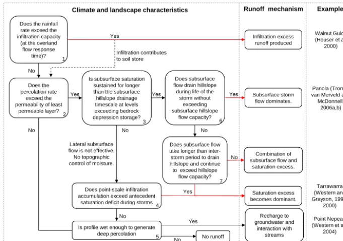
To aid systematic consideration of the variation in runoff processes between catchments and over time, we develop a summary of the status quo in terms of the combined effects of thresholds and connectivity on runoff processes at the hill-slope to zero-order catchment scale (Fig. 1). Often we think of dominant runoff processes and, as Fig. 1 is easiest to in-terpret in that context, the following discussion takes that view initially. However, there is often a mix of runoff pro-cesses either spatially due to heterogeneity or for different events, and Fig. 1 can also be used to interpret such a mixture, which we will return to later. This paper aims to tease apart the influence of different processes by considering 60 rain-fall events (resulting in 38 runoff events) in a small agricul-tural catchment. We show the shifting importance of differ-ent processes over time associated with changes in catchmdiffer-ent wetness and rainfall intensity and apply the runoff process framework. We consider the role of thresholds in different catchment states and fluxes as well as the role of thresholds in certain timescales in controlling different modes of hydro-logic connectivity and associated rainfall–runoff responses. The variety of potential thresholds leads to a variety of runoff processes, as illustrated in the following discussion.
Yes
Panola (Tromp-van Merveld and
McDonnell, 2006a,b) Runoff mechanism
Climate and landscape characteristics
Does subsurface flow drain hillslope
during life of the storm without
exceeding subsurface hillslope
flow capacity? Does the rainfall
rate exceed the infiltration capacity
(at the overland flow response
time)?
Does the percolation rate
exceed the permeability of least
permeable layer?
Recharge to groundwater and
interaction with streams No
Is subsurface saturation sustained for longer than the subsurface hillslope drainage timescale at levels exceeding bedrock depression storage? Yes
No
Lateral subsurface flow is not effective.
No topographic control of moisture.
Infiltration excess runoff produced Infiltration contributes
to soil store
No
Subsurface storm flow dominates. Yes
Saturation excess becomes dominant. Yes
Does subsurface flow take longer than inter-storm period to drain hillslope and continue to exceed hillslope
flow capacity?
Yes
Combination of subsurface flow and
saturation excess. Yes
No
No
Does point-scale infiltration accumulation exceed antecedent
saturation deficit during storms No 1
2
3
4
6
7
Example
Tarrawarra (Western and Grayson, 1998,
2000) Point Nepean (Western et al.,
2004) Is profile wet enough to generate
deep percolation 5
Walnut Gulch (Houser et al,
2000)
[image:3.612.128.469.67.306.2]No runoff No
Figure 1.The role of flux and timescale thresholds in determining runoff processes. The red lines indicate cases where there is surface or subsurface hillslope connectivity to the stream.
to represent the competing effects of transport and reaction timescales on the loss of material along a flow path. When the reaction timescale is small compared with the transport timescale, the reactant is consumed before reaching the exit of the flow path it is moving along. A complication here is that both flux and time thresholds are important. This arises because there is finite capacity for flow in various parts of the catchment system.
Figure 1 is divided into three parts; the left-hand area pro-vides a series of catchment thresholds that depend on hy-droclimatic and landscape characteristics and influence the type of runoff process and the connectivity between the hill-slope and stream, depending on whether they are exceeded or not. The middle area points to the outcome in terms of dominant runoff generation processes and the right-hand area provides example catchments from the literature that exhibit those processes. In Fig. 1 we define the specific runoff pro-cesses as follows.
Infiltration excess runoff: runoff that occurs due to the rainfall (or throughfall) rate exceeding the infiltration capac-ity of the surface and that results in flows of water to the catchment outlet by surface flow pathways.
Subsurface stormflow: runoff due to infiltration that gener-ates rapid lateral subsurface flow (i.e. a quickflow response) that flows to the catchment outlet through subsurface flow paths for at least part of the distance to the outlet. This wa-ter may exfiltrate in low convergent parts of the catchment or directly into the stream before reaching the catchment outlet. Often impeding layers and preferential flow paths are impli-cated.
Saturation excess runoff: runoff due to rainfall on saturated areas that flows to the catchment outlet by surface flow path-ways. The saturated area may be generated by either lateral flow in excess of the capacity of the hillslope to transmit the lateral flow, a drainage impediment at depth coupled with a sufficient excess of infiltration over evapotranspiration and drainage, or a combination of these.
Some of the thresholds are posed in terms of flux rate com-pared with a flow capacity (e.g. box 2) and some in terms of a state threshold (box 5). The flux and state thresholds are con-sidered in the context of process timescales and durations. This is because the threshold needs to be exceeded for a suffi-cient time for the action of the process to lead to a significant impact. That impact typically involves lateral flow either on the surface or through the subsurface and hence also inter-actions upslope and downslope. Specific examples are given below.
celerity) is important. The remaining boxes consider thresh-olds in the context of subsurface flow times. Box 3 con-siders situations where subsurface saturation exists, allow-ing water to flow along lateral subsurface flow paths. If any one of deep infiltration through the impeding layer (Jackson et al., 2014), unfilled bedrock storage (Janzen and McDon-nell, 2015) or evapotranspiration (including between events) causes the saturation and/or lateral flow to cease before water can move a significant distance downstream, the water will not be effectively redistributed downslope, and subsurface connection will not be established. If the saturation persists for long enough for lateral subsurface flow to move down the hillslope and into the stream, connectivity between the hills-lope and the stream will develop. Thus the ratio of the lateral flow timescale for the hillslope and the evaporative drying (or other loss) timescale is important here. At the other ex-treme (box 7), if lateral flow is persistently exceeding the subsurface flow capacity, surface saturation will exist, lead-ing to saturation excess runoff because saturated areas will exist antecedent to the event in this case. Provided continu-ous saturation exists to the stream, this will lead to a surface flow path connecting the hillslope and stream. In this case the lateral flow timescale is long enough to lead to memory in the spatial patterns between events (non-local control of Grayson et al., 1997).
While Fig. 1 suggests catchment rainfall–runoff response is dominated by specific processes (e.g. saturation excess runoff), it needs to be recognised that many catchment con-ditions vary over time and space. For example, in our study, catchment summer rainfall is often more intense than win-ter rainfall, and this can lead to differences in runoff pro-cesses between events. Soil water conditions vary seasonally in response to both rainfall and potential evapotranspiration, sometimes leading to switching between characteristic spa-tial patterns of soil moisture and prevailing responses to rain-fall (Grayson et al., 1997; Western et al., 1999). Topographic, soil and vegetation conditions can also vary across a catch-ment. This all suggests that catchments could exhibit a mix of processes.
Having introduced the framework above, we use it to un-derstand the behaviour of a catchment in Australia that does indeed exhibit a mix of runoff processes. We examine how soil water storage and shallow water table response influence surface and subsurface connectivity and rainfall–runoff re-sponse at seasonal and event based timescales. We also ex-amine the relative role of saturation excess and subsurface flow in generating peak runoff rates and event volumes. Fi-nally we examine circumstances under which rainfall inten-sity plays a role in runoff generation responses. The field site is a small agricultural catchment in the Lang Lang River catchment, Victoria, Australia, which we examine through the lens of hydrometric and isotope and geochemistry mea-surements. In the context of Fig. 1, these results are used to examine various runoff generation mechanisms and flow pathways that are important in the study catchment and to
de-termine how they contribute to produce the catchment runoff as the catchment wetness and rainfall intensity vary. Thus the contributions of this paper revolve around the introduction of the framework in Fig. 1 and demonstration of its applica-tion using a catchment where multiple runoff processes are important. The paper also contributes to further understand-ing of the role of thresholds and connectivity in determin-ing flow pathways and runoff processes in agricultural catch-ments. Most connectivity studies in the past have focussed on forested catchments.
2 Methods 2.1 Study location
The study site is a 1.37 ha catchment (named RBF) located on a dairy farm at Poowong East, in the Lang Lang River catchment, Victoria, Australia, 130 km south-east of Mel-bourne (Fig. 2). The study area has a humid climate and rainfall is uniformly distributed across the year, with an an-nual mean (1961–1990) of 1100 mm (Bureau of Meteorol-ogy, 2009). Annual areal potential evapotranspiration (1961– 1990) is 1040 mm (Bureau of Meteorology, 2005).
A general description of the study catchment can be found in Adams et al. (2014). The study period was between September 2009 and December 2011. Elevation ranges from 160 to 210 mAHD (Australian Height Datum) and the slope varies from 2 to 50 %. Based on field observations, the to-pography, range of slopes and the groundwater behaviour, the catchment was divided into four different zones: (1) the riparian area located on the relatively flat convergent lower part of the catchment (outlined in red in Fig. 2) included sites 1, 2, 32 and 3; (2) the lower slope (low slope) area; (3) the mid-slope area with sites 4, 5, 6 and 7; and (4) the upper slope (upslope) area with sites 10, 11 and 15 (Fig. 2).
The catchment geology comprises sandstones and mud-stones of the Cretaceous Strezlecki Group (VRO, 2013). Out-crops on the lower stream banks of the catchment (just down-stream of the monitored hillslope) show weathered sandstone and mudstone bedrock. Hand augering revealed a soil depth of between 1 and 1.6 m, and the lower parts of the profile included mottled clay and weathered bedrock particles. The soils are acidic and mesotrophic brown dermosols (Isbell, 2002) that grade from a fine sandy clay loam to a medium clay with mottles and weathered bedrock. Soil profile depth decreases, moving downslope. These soils typically have a moderate hydraulic conductivity surface horizon (0–40 cm,
Ks ≈5×10⁻⁶m s−1, about 20 mm h−1). The dominant land
use is grazing by dairy cows.
2.2 Site instrumentation and hydrometric data monitoring
!
!
! !
!
! !
! !
!
!
!
#
!
Lower slope
Middle slope
Upper slope
185 180
175
170
190 165
195 160
200
205 AWS 4
5 6 3
7 2 1 16
32
15
11 10
±
^ ! Melbourne
Study area
Legend
! Wells
Main stream Drainage lines
Riparian zone
#
Flume
[image:5.612.154.441.69.223.2]0510 20m
Figure 2.The study site location within Australia and a hill shaded DEM, topography and sampling site locations at RBF. In this figure the black circles show shallow groundwater sites, the red circle shows the soil moisture site and the blue triangle demonstrates the catchment flume.
15-04-1013-05-1010-06-1008-07-1005-08-1002-09-1030-09-1028-10-1025-11-1023-12-1020-01-1117-02-1117-03-1114-04-1112-05-1109-06-1107-07-1104-08-1101-09-1129-09-1127-10-1124-11-11
Weekly rainfal (mm)
0 20 40 60 80 100
Rainfall
Weekly APET (mm)
0 10 20 30 40 50
(a)
APET
15-04-1013-05-1010-06-1008-07-1005-08-1002-09-1030-09-1028-10-1025-11-1023-12-1020-01-1117-02-1117-03-1114-04-1112-05-1109-06-1107-07-1104-08-1101-09-1129-09-1127-10-1124-11-11
Soil water storage (mm)
150 180 210 240 270 300
Soil water storage
Weekly runoff (mm)
0 10 20 30 40 50
(b)
Runoff
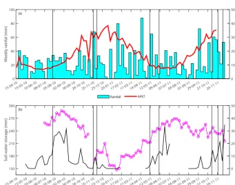
Figure 3. (a)Weekly rainfall and APET (areal potential evapotranspiration) time series,(b)soil water storage in the top 60 cm of the soil profile and weekly runoff time series for the flume at the catchment outlet. The rainfall, areal potential evapotranspiration and volumetric soil moisture used to calculate soil moisture storage were all recorded at the AWS (automatic weather station) (Fig. 1). The vertical bars show the timing of events in Fig. 4.
Odyssey (Dataflow Systems inc. Christchurch, NZ) pressure transducer (PT) recorded stream water levels every 10 min, which were used to compute instantaneous discharge rates. After August 2011, the PT was replaced with an ISCO (Tele-dyne ISCO, Lincoln, NE, USA) model 730 bubbler. The fol-lowing rating curve was used to calculateQfrom water level:
Q=0.001H2+0.0168H, (1)
[image:5.612.128.470.278.547.2]seasonal, resulting in strongly seasonal soil moisture con-tents and intermittent streamflow at RBF. Soil moisture stor-age was calculated from the volumetric soil water content which was measured for the 0–30 and 30–60 cm layers and recorded hourly by the AWS logger using two vertically in-stalled 30 cm long Campbell Scientific (CS625) soil moisture probes (Campbell Scientific, 2006). The 0–30 cm probe was inserted from the surface. To install the 30–60 cm probe, a 30 cm deep hole was dug, with the excavated soil set aside. The probe was inserted vertically and then the excavated soil was repacked so that the soil was replaced at a similar depth to that from which it had been removed.
The CS625 produces a pulse signal and the pulse period was temperature corrected using measured soil temperature, and the manufacturers recommended temperature correction, as follows (Campbell Scientific, 2006).
τcorrected(Tsoil)=τuncorrected+(20−Tsoil) (2) ·0.526−0.052·τuncorrected+0.00136·τuncorrected2 ,
whereτuncorrectedis the probe output period,Tsoil is the soil
temperature andτcorrectedis the corrected probe output. The VWC was then computed from τcorrected using (Campbell Scientific, 2006)
VWC= −0.0663−0.0063·period+0.0007·period2. (3) Soil water storage over the top 60 cm soil depth was com-puted by adding the VWC from the 0–30 and 30–60 cm lay-ers and then multiplying by the 300 mm soil depth. We use this soil water storage at the start of each rainfall event as an index of antecedent soil water (ASI) and assume it represents the catchment wetness condition.
To capture the nature of hydrologic connectivity, runoff mechanisms and flow pathways, shallow (1.5–1.6 m) ground-water wells were installed at 12 sites across the RBF catch-ment using 40 mm PVC pipes and backfilled with sand, ben-tonite, the topsoil and grass. Figure 2 shows these sites, of which 1, 2, 3, 16 and 32 were in the riparian zone; 4, 5, 6 and 7 were on the mid-slope; and 10, 11 and 15 were on the upper slope. Sites 4, 5 and 6 were equipped with water level loggers from July 2010 until the end of study period in De-cember 2011. Sites 3, 7, 16 and 32 were logged from winter 2011 until the end of the study period in December 2011. Wa-ter level loggers were not installed at sites 1 and 2 since they were nearly always saturated. At sites 1 and 2 groundwater levels were measured manually. Water levels were logged us-ing Odyssey PT loggers.
2.3 Water sampling and analysis
A rainfall sampler (Kennedy et al., 1979) collected up to 10 sequential rainfall samples per event, each being equiva-lent to 6.6 mm of rainfall. The sampler was initially installed close to the AWS; however, due to instances of damage by
animals, it was relocated near to the flume in August 2010 until the end of the study period (December 2011).
An auto sampler (Teledyne ISCO 6712) was installed at the flume and streamflow sampling was triggered based on the rising stage. Following triggering, the sampler was programmed to collect up to 24 samples of streamflow at hourly intervals. Samples were removed from the auto sam-pler within 48 h. To reduce the laboratory analysis workload, we plotted recorded water levels from the RBF catchment in the field prior to removing the event sample from the auto sampler and selected certain samples for analysis. All sam-ples during the rising limb and the peak were selected and samples were typically selected at an interval of 4 h during the falling limb. Routine grab sampling was undertaken at weekly intervals during the main runoff season when water was flowing through the RBF flume. This was supplemented by additional grab sampling during visits to collect event samples from the auto sampler. Routine grab sampling was also undertaken at weekly intervals during the main runoff season when water was flowing through the RBF flume.
Sub-samples for isotopic analysis were taken of stream water from both manual and auto sampler samples, and from all full rainfall sample bottles; these were collected in glass bottles for isotope analysis. Bottles were completely filled. The samples were refrigerated (+4◦C) until analysis for δ18O andδ2H. Stable isotope ratios were measured ei-ther at Monash University using a Finnigan MAT 252 and ThermoFinnigan Delta Advantage Plus mass spectrometers (2010 samples) or at the University of Melbourne, where a Picarro L2120i cavity ring-down isotope analyser was used to determine isotope ratios (2011 samples). The instrumen-tal precision wasδ18O= ±0.15 ‰ andδ2H= ±1 ‰ for the isotope samples analysed at Monash University, and it was
δ18O=0.1 ‰ andδ2H=0.4 ‰ for samples analysed at Mel-bourne University. The results from the isotope analysers were checked for systematic differences, by analysing du-plicate samples in both laboratories. We developed and ap-plied a correction between the two laboratories based on these samples. With the exception of determining pre-event end member uncertainty (described later), the analyses pre-sented here only use samples analysed at the Monash labo-ratory, and hence this difference between laboratories only affects our hydrograph separation uncertainty estimates. For isotope analysis, in total we collected 115 samples of rain-fall, 28 samples during low flows and multiple stream water samples of isotopes from five events.
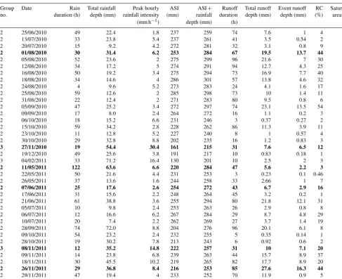
Table 1.Rainfall–runoff event summary at RBF. ASI is the Antecedent Soil moisture Index. RC is the quickflow runoff coefficient. Runoff event grouping is discussed in Sect. 3.2. The events in bold are shown in Fig. 4.
Group Date Rain Total rainfall Peak hourly ASI ASI+ Runoff Total runoff Event runoff RC Saturated no. duration (h) depth (mm) rainfall intensity (mm) rainfall duration depth (mm) depth (mm) (%) area (%)
(mm h−1) depth (mm) (h)
2 25/06/2010 49 22.4 1.8 237 259 74 7.6 1 4 4.5
2 13/07/2010 33 23.8 5.4 237 261 41 3.5 0.54 2
2 20/07/2010 15 9.2 4.2 272 281 32 3.1 0.8 9 5.3
2 01/08/2010 30 31.4 6.2 253 284 67 19.5 13.7 44 5.5
2 05/08/2010 52 23.6 2 275 299 96 21.6 7 30 5.5
2 12/08/2010 34 17.2 5 274 291 94 12.7 4.3 25 5.5
2 16/08/2010 50 19.2 3.4 275 294 73 16.9 7.7 40 5.5
2 18/08/2010 34 14.6 4 286 301 57 13.8 4.6 32 5.5
2 24/08/2010 4 9.6 5.2 273 283 24 4.1 1.6 17 5.5
2 25/08/2010 59 12.6 2 285 298 73 10 1.4 11 5.5
2 31/08/2010 22 12.4 2 271 283 80 9.5 0.8 6 5.5
2 05/09/2010 47 25.2 3.4 272 297 74 23.1 13.5 54 5.5
2 09/09/2010 17 8.0 2.4 264 272 16 1.1 0.2 3 5.3
2 06/10/2010 18 15.2 6.6 231 246 3 0.37 0.27 2 NA
2 15/10/2010 59 34.2 2.8 228 262 86 11.3 3.9 11 NA
2 23/10/2010 11 12.8 5.2 227 240 8 1 0.57 4 NA
2 30/10/2010 29 32.8 8.8 202 235 16 1.2 0.83 3 NA
3 27/11/2010 19 54.4 30.4 161 215 31 7.6 6.5 12 NA
2 19/12/2010 49 25.6 3.8 191 217 10 0.83 0.18 1 NA
3 04/02/2011 33 71.2 16.4 130 201 10 2.5 2 3 NA
2 11/05/2011 122 63.6 6.6 220 284 47 5.6 2.2 3 NA
2 22/05/2011 50 21.6 4.4 231 253 3 0.23 0.1 0.46 NA
2 26/05/2011 37 13.6 1.6 244 258 33 2.66 1 7 NA
2 07/06/2011 25 17.6 2.6 254 272 43 6.7 2.9 16 NA
2 17/06/2011 31 15.6 2.2 248 264 45 3.2 0.2 1 4.6
2 21/06/2011 61 38.8 3.6 255 294 80 21.8 12.1 31 4.6
2 05/07/2011 10 9.8 2.4 253 263 26 2.9 0.8 8 4.7
2 06/07/2011 12 16.6 6.2 267 284 29 8.7 4.8 29 4.7
2 10/07/2011 20 7.4 2.2 262 269 27 3.7 1.4 19 4.7
2 28/09/2011 74 72.0 8.8 204 276 96 20.1 6.1 8 5.4
2 09/10/2011 54 23.2 2.4 232 255 5 0.35 0.14 1 NA
2 28/10/2011 19 30.2 7.8 213 243 6 0.92 0.6 2 NA
3 08/11/2011 12 35.2 14.8 222 257 31 10 7.1 20 5.2
2 09/11/2011 14 23.8 6.8 239 263 44 15.7 8.9 37 5.2
2 18/11/2011 30 45.5 10.2 219 265 82 17.7 8.9 20 5.5
2 26/11/2011 29 36.8 8.4 216 253 85 27.6 16.3 44 5.5
2 29/11/2011 47 19.4 4 233 252 70 11.9 0.9 5 5.5
3 10/12/2011 16 52.6 31 192 245 32 41.1 35.6 68 5.5
Group 2 has ASI+Rain > 250 mm; Group 3 hasIpeak> 15 mm h−1. “NA” stands for “not available”.
– Mg2+was determined by atomic absorption spectrom-etry (APHA, 2005). The issue of interference with Si, Al, and P was solved using a combination of lanthanum and caesium. The determined uncertainty for Mg2+was Cm·0.0596, with a 95 % confidence interval (CI). – Ca2+ was analysed using atomic absorption
spec-trometry utilising an air/acetylene flame based on the American Public Health Association procedure (APHA, 2005). The issue of interferences with Si, Al, and P was solved using lanthanum releasing agents. The de-termined uncertainty for Ca2+ was Cm·0.0386 (95 % CI).
– Following the APHA (2005) approach, “flame atomic absorption spectrometry” was used to determine K+
concentration and caesium was used to solve the issue of ionisation. Uncertainty for K+ was Cm·0.0372 (95 % CI).
– Na+which is “ionized in the air/acetylene flame” was analysed by adding caesium to overcome this prob-lem following the APHA (2005) method. Uncertainty in Na+results was Cm·0.0432 (95 % CI).
2.4 Rainfall and runoff events
In order to analyse event behaviour, it was necessary to identify rainfall and runoff events. Based on an exami-nation of the time series of hourly rainfall in the catch-ment (in the study period which was between April 2010 and December 2011), rain events were defined as hav-ing >=5 mm total rainfall, and peak hourly rainfall inten-sity,Ipeak>=1.5 mm h−1. Distinct events were separated by
> 12 h without rainfall.
The runoff hydrograph was also divided into events. Runoff events began when the stream discharge hydrograph started to rise from its initial low flow value or moved above a threshold of 0.05 mm h−1following the commencement of a rainfall event. Events ended either when (1) the discharge returned to its initial value, (2) a new rainfall event started, or (3) 96 h after the end of the rainfall event in unusually wet situations where elevated flow continued. For each event, a number of characteristics were determined as shown in Ta-bles 1 and 2.
The Antecedent Soil moisture Index (ASI) was repre-sented as the amount of the soil water storage in the top 60 cm of the profile at the AWS at the start of each rainfall event. The topography of the catchment was surveyed using a dif-ferential Global Positioning System (dGPS) and a 1 m hori-zontal resolution DEM (digital elevation model) was devel-oped by interpolation methods. Instrument and well locations were also determined using dGPS. Then these data were used to produce maps of the study area, including sampling sites using Arc GIS. The lateral boundary of the saturated area was topographically constrained and field inspections suggested it was stable over time, while the upstream boundary moved up and down the riparian zone. The saturated area was esti-mated by locating the upper boundary through field inspec-tion and then measuring the distance from either well 2 or 3 (the saturated area extended towards site 3 during very wet conditions). Figure 2 demonstrates the approximate maxi-mum boundary location of the saturated area at site 3 and the main stream located close to the outlet of the catchment. The saturated area was then estimated from this information com-bined with the mapping of the riparian zone boundary in Ar-cGIS. These measurements were made between events. The proportion of saturated area was estimated using these data and then used to estimate saturation excess runoff genera-tion for the different events. Consistent with our definigenera-tions in Fig. 1, here we conceptually separate return flow and flow re-sulting from direct precipitation on the saturated area and use saturation excess runoff to refer to the latter. The event runoff depth (mm) and event runoff coefficient (RC %) were calcu-lated by separating the event hydrograph using the method of Hewlett and Hibbert (1967), which has been widely applied (Buttle et al., 2004; Fujimoto et al., 2008; McGuire and Mc-Donnell, 2010). The method assumes that baseflow increases at the rate of 0.55 L s−1km−2h−1(0.002 mm h−1) from the start of the rising limb. While this method, like other
hydro-graph based baseflow separation methods, is arbitrary, the re-sults are insensitive to the assumed rate of rise.
2.5 Isotopic hydrograph separation
Isotope samples are used for hydrograph separation into pre-event and event contributions. We applied the well-known one-tracer, two-component model of hydrograph separation approach (Pinder and Jones, 1969; Sklash and Farvolden, 1979). We determined uncertainties following Genereux (1998). We undertook the analysis using both the
2H and18O data. We used the mean of the rainfall samples
during the event to estimate the event water end member and low flow samples from the few days to the event for the pre-event end member. In the uncertainty analysis, the standard deviations of the event rainfall samples and of all the low flow samples across the study period were used. Half the analytic uncertainty was used to represent the standard deviation of the streamflow sample.
3 Results
The following results first provide an overview of the sea-sonal behaviour and rainfall–runoff events. They then exam-ine whether thresholds in the antecedent conditions and/or event rainfalls exist. Next, links between the catchment con-dition and the event runoff are examined using the piezome-ter and soil moisture data. Afpiezome-ter that, the recession behaviour of events is examined and linked to catchment wetness con-ditions. Finally, isotope and major ion data are presented for selected events.
3.1 Overview of runoff behaviour and rainfall–runoff event characteristics
Figure 3 shows time series of weekly rainfall, APET, soil wa-ter storage and runoff. The rainfall, although variable from week to week, exhibited seasonality, while there was strong seasonality in PET. This drove a strong seasonality in soil water storage. An examination of the weekly runoff data shows that there was generally no flow from about October to May due to the seasonal nature of this catchment; how-ever, an exception was that persistent low flow occurred from 26 November 2011 to the end of the event on 10 Decem-ber 2011. During this period the ASI was often relatively low, but there was frequent and substantial rainfall (> 200 mm in 30 days). While a strong link between runoff and soil water storage is evident at the seasonal scale in Fig. 3, there are ex-ceptions at the event scale. For example, in February 2011, there was runoff response despite the catchment being near to the lowest soil water storage for the study period.
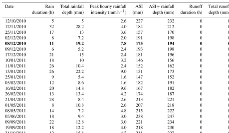
Table 2.Rainfall event summary at RBF with no runoff (Group 1 events). ASI is the Antecedent Soil moisture Index. The events in bold are shown in Fig. 4.
Date Rain Total rainfall Peak hourly rainfall ASI ASI+rainfall Runoff Total runoff
duration (h) depth (mm) intensity (mm h−1) (mm) depth (mm) duration (h) depth (mm)
12/10/2010 5 5 2.6 227 232 0 0
12/11/2010 32 28.2 4.0 184 212 0 0
25/11/2010 17 13 3.6 157 170 0 0
02/12/2010 8 7.2 2.0 191 198 0 0
08/12/2010 11 19.2 7.8 175 194 0 0
09/12/2010 6 5.2 2.4 193 198 0 0
17/12/2010 21 15 2.4 181 196 0 0
10/01/2011 18 10 3.2 146 156 0 0
11/01/2011 26 10.4 2.4 152 162 0 0
13/01/2011 26 22.2 9.0 151 173 0 0
25/01/2011 9 5.4 1.6 147 152 0 0
05/02/2011 12 8.6 1.6 182 191 0 0
16/02/2011 20 14.8 9.6 167 182 0 0
26/02/2011 13 13.4 4.2 174 187 0 0
21/04/2011 28 8.4 2.6 213 221 0 0
01/05/2011 8 10.8 2.6 207 218 0 0
08/05/2011 14 7.2 4.8 215 222 0 0
05/06/2011 18 9.4 3.0 238 247 0 0
09/09/2011 22 12.8 3.0 221 234 0 0
19/09/2011 18 12.2 4.0 218 230 0 0
24/10/2011 12 15.6 4.2 211 227 0 0
are not included in the analysis due to missing stream dis-charge data. For the 38 runoff events, total event rainfall var-ied from 7 to 72 mm,Ipeakranged from 2 to 31 mm h−1, the
ASI ranged from 130 to 286 mm and total event runoff varied between 0.23 and 41 mm. For the no-flow events (Table 2), total rainfall varied from 5 to 28 mm,Ipeakranged from 2 to
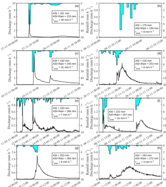
10 mm h−1 and the ASI ranged from 146 to 238 mm. Fig-ure 4 shows rainfall–runoff responses for selected events at RBF. These graphs are ordered from lowest (27 Novem-ber 2010) to highest ASI (7 June 2011) for the selected events. All events (except events on 26 November 2011 and 10 December 2011; Fig. 4c) presented in Fig. 4 had zero or very low initial flow. For the events on 26 November 2011 and 10 December 2011, the initial discharge was 0.07 and 0.13 mm h−1, respectively.
In Fig. 4 most events showed rapid response to rainfall, except for the event on 8 December 2010 (Fig. 4b), which did not produce any significant runoff, and the event on 7 June 2011. The events on 27 November 2010 and 10 De-cember 2011 in particular showed a very flashy response. These events had the highest peak hourly rainfall intensity (30.4 and 31 mm h−1, respectively) during the study period, and they occurred at the end of the flow season with low ASI (ASI was 161 and 192 mm, respectively). The highest peak runoff rates for the study period were for the events on 27 November 2010 and 10 December 2011, which were 2.4 and 5.6 mm h−1, respectively. In contrast to most events, the runoff response for the event on 27 November 2010 was
tran-sient with very rapid recession. For the event on 10 Decem-ber 2011, a second peak of moderate rainfall intensity (about 10 mm h−1) produced a second runoff peak, and there was a more significant recession flow following the rainfall bursts. This was also true for the other events (8 and 26 Novem-ber 2011, 11 May 2011, 1 August 2010, 7 June 2011) shown in Fig. 4, which were typical of responses to lower intensity rainfall during wetter (in terms of soil water) periods.
For events with Ipeak< 10 mm h−1 there was a general
increase in response as the ASI increased. The event on 12 November 2010 had 184 mm ASI and total rainfall was 28 mm, and it did not produce any runoff. This was a typi-cal example of no-flow events. Coming into the runoff sea-son, as the ASI increased (e.g. 220 mm on 11 May 2011), RBF started to respond gradually, producing small amounts of runoff (e.g. for events on 11 and 14 May 2011). When the ASI was > 250 mm for the event on 7 June 2011, it can be clearly seen that RBF responded to this low intensity, small size rainfall event with a delayed and smooth discharge hy-drograph with continued flow following the event. This also occurred for the next event on 1 August 2010.
3.2 Runoff thresholds
Rainfall (mm h -1) 0 10 20 30 40 50
27-11-10 06:00 27-11-10 18:00 28-11-10 06:00 28-11-10 18:00
Discharge (mm h -1) 0 2 4 6 8 10 (a)
ASI = 161 mm ASI+Rain = 215 mm Ipeak = 30 mm h-1
Rainfall (mm h -1) 0 2 4 6 8 10
08-12-10 00:00 08-12-10 12:00 09-12-10 00:00 09-12-10 12:00
Discharge (mm h -1) 0 0.2 0.4 0.6 0.8 1 (b)
ASI = 175 mm ASI+Rain = 194 mm Ipeak = 8 mm h-1
Rainfall (mm h -1) 0 10 20 30 40 50
10-12-11 06:00 10-12-11 18:00 11-12-11 06:00 11-12-11 18:00
Discharge (mm h -1) 0 2 4 6 8 10 (c)
ASI = 192 mm ASI+Rain = 245 mm Ipeak = 31 mm h-1
Rainfall (mm h -1) 0 4 8 12 16 20
26-11-11 00:0026-11-11 12:0027-11-11 00:0027-11-11 12:0028-11-11 00:0028-11-11 12:0029-11-11 00:00
Discharge (mm h -1) 0 0.4 0.8 1.2 1.6 2 (d)
ASI = 216 mm ASI+Rain = 253 mm Ipeak = 8 mm h-1
Rainfall (mm h -1) 0 2 4 6 8 10
11-05-11 00:0012-05-11 00:0013-05-11 00:0014-05-11 00:0015-05-11 00:0016-05-11 00:0017-05-11 00:00
Discharge (mm h -1) 0 0.2 0.4 0.6 0.8 1 (e)
ASI = 220 mm ASI+Rain = 284 mm Ipeak = 7 mm h-1
Rainfall (mm h -1 ) 0 4 8 12 16 20
08-11-11 00:0008-11-11 12:0009-11-11 00:0009-11-11 12:0010-11-11 00:0010-11-11 12:0011-11-11 00:00
Discharge (mm h -1) 0 0.4 0.8 1.2 1.6 2 (f)
ASI = 222 mm ASI+Rain = 257 mm Ipeak = 15 mm h-1
Rainfall (mm h -1) 0 6 12 18 24 30
01-08-10 00:0001-08-10 12:0002-08-10 00:0002-08-10 12:0003-08-10 00:0003-08-10 12:0004-08-10 00:00
Discharge (mm h -1) 0 0.6 1.2 1.8 2.4 3 (g)
ASI = 253 mm ASI+Rain = 284 mm Ipeak = 6 mm h
-1 Rainfall (mm h -1) 0 2 4 6 8 10
07-06-11 00:0007-06-11 12:0008-06-11 00:0008-06-11 12:0009-06-11 00:0009-06-11 12:0010-06-11 00:00
Discharge (mm h -1) 0 0.2 0.4 0.6 0.8 1 (h)
ASI = 254 mm ASI+Rain = 272 mm Ipeak = 3 mm h
[image:10.612.133.466.66.442.2]-1
Figure 4.Characteristics of eight selected rainfall–runoff events sorted by their Antecedent Soil moisture Index (ASI). Rainfall is shown in blue. It should be noted that the axis scales vary between events. All events (except those on 26 November and 10 December 2011) had
zero or very low initial discharge. For the events on 26 November and 10 December 2011, the initial discharges were 0.07 and 0.13 mm h−1,
respectively. Note that the axes vary between events.
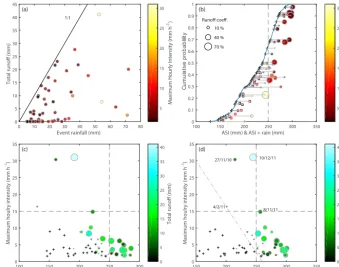
builds on approaches by Detty and McGuire (2010), who considered thresholds in ASI and ASI+Rain (i.e. Fig. 5c and d), and Janzen and McDonnell (2015), who considered the impact of event rainfall and rainfall intensity on event runoff (i.e. Fig. 5a). As we move from Fig. 5a to d, the var-ious influences on rainfall–runoff behaviour and thresholds become clearer. Figure 5a shows event runoff as a function of event rainfall, with the highest hourly rainfall intensity (Ipeak) indicated in colour. This illustrates that there is
lit-tle relationship between event rainfall and runoff or between rainfall intensity and runoff. For some quite large events (up to∼25mm), zero runoff can occur. There was also a wide variation in runoff coefficients (indicated by the scatter). It is also clear that the events with high peak hourly intensity also had relatively large total rainfall accumulations. Over-all, Fig. 5a shows that event rainfall and intensity do not
effectively differentiate rainfall–runoff behaviour when con-sidered by themselves.
Figure 5b begins to separate out different effects by show-ing the impact of five factors together. The cumulative curve shows the distribution of soil water storage as observed throughout the study period. Specific events are shown with the ASI identified (left-hand end of the grey lines) and the ASI+Rain depth (filled markers at the right end of the hori-zontal grey lines). The length of the lines is the rainfall depth for the event. The colour of each bubble shows the peak hourly rainfall intensity (Ipeak) and the size of the bubbles
Event rainfall (mm)
0 10 20 30 40 50 60 70 80
Total runoff (mm)
0 5 10 15 20 25 30 35 40 45 1:1
Maximum Hourly Intensity (mm h
-1) 5 10 15 20 25 30
ASI (mm) & ASI + rain (mm)
100 150 200 250 300 350
C u m u la tiv e pro b a b lili ty 0 0.1 0.2 0.3 0.4 0.5 0.6 0.7 0.8 0.9 1 Runoff coeff. 10 % 40 % 70 % Maximum hourly intensity (mm h ) -1 5 10 15 20 25 30 ASI (mm)
100 150 200 250 300
Maximum houlry intensity (mm h ) -1 0 5 10 15 20 25 30 35
Total runoff (mm)
0 5 10 15 20 25 30 35 40
ASI + rain (mm)
150 200 250 300 350
Maximum houlry intensity (mm h ) -1 0 5 10 15 20 25 30 35 27/11/10 10/12/11 4/2/11 8/11/11
Total runoff (mm)
[image:11.612.130.469.67.334.2]0 5 10 15 20 25 30 35 40 (a) (b) (c) (d)
Figure 5.Thresholds of runoff mechanisms at RBF.(a)Event rainfall vs. event total runoff, colours indicating the highest hourly rainfall
intensity.(b)The impact of five factors together, including the cumulative curve of the distribution of soil water storage as observed through
the study period, ASI, ASI+Rain; colour shows the peak hourly rainfall intensity (Ipeak) and the size of the bubbles shows the event runoff
coefficient.(c)ASI vs. the peak hourly rainfall intensity (Ipeak), and the size of the bubbles shows the event runoff coefficient and colour
shows event total runoff.(d)ASI+Rain vs. the peak hourly rainfall intensity (Ipeak), and the size of the bubbles shows the event runoff
coefficient and colour shows event total runoff. Note that ASI is the antecedent soil water storage (mm) in the top 60 cm of the soil at the AWS at the beginning of the event.
ASI+Rain=250 mm (right-hand end of the horizontal grey line).
There are several trends that can be discerned from Fig. 5b. First the rainfall events analysed here occurred across the full range of catchment wetness and were relatively evenly spread, showing that the rainfall events occur over a rep-resentative range of catchment antecedent conditions. The larger rainfall events generally occurred in summer when ASI < 250 mm and a mix of low and high intensity events occurred for these conditions, also in summer. All the events on a wet catchment (ASI > 250 mm) had low Ipeak
(≤6.2 mm h−1). Events where the ASI+Rain was less than 250 mm usually did not generate any runoff, although there were some high intensity rainfall events that were exceptions and a small number of events with very low runoff coeffi-cients (1–4 %) where the ASI+Rain was generally between 230 and 250 mm. These low runoff coefficient events were at the end of the runoff season.
Figure 5c and d examine the impact of catchment wetness, quantified as ASI and ASI+Rain, respectively, at the start (Fig. 5c) and end (Fig. 5d) of the event, on event runoff response, combined with the impact of rainfall intensity,
Ipeak. Catchment wetness is plotted on thex axis and
rain-fall intensity on they axis. Values ASI=250 mm (Fig. 5c), ASI+Rain=250 mm (Fig. 5d) and Ipeak=15 mm h−1 are
shown by grey dashed lines. The bubble size shows the event runoff coefficient, as before, and crosses indicate rainfall events that did not generate any runoff. Colour indicates the runoff volume. The runoff coefficient behaviour is separated into groups more clearly in Fig. 5d than in Fig. 5c. In Fig. 5d, three different groups of events can be identified. Looking along thexaxis, there is a threshold at ASI+Rain=250 mm that separates most events with a significant runoff response from those without. Looking along they axis direction, it can be seen that the ASI+Rain threshold is not success-ful at distinguishing runoff when Ipeak is high and there is
also a threshold in runoff response at Ipeak=15 mm h−1.
Thus the three groups are (1) events without runoff where ASI+Rain < 250 mm andIpeak< 10 mm h−1, (2) events that
produce runoff when ASI+Rain > 250 mm and (3) events with ASI+Rain < 250 mm and Ipeak> 15 mm h−1 that did
produce runoff (Tables 1 and 2). Where ASI+Rain exceeded 250 mm (group 2), some runoff was always produced.
rainfalls mostly happened in drier periods when ASI varied between 146 and 227 mm. It is assumed that rainfall com-pletely infiltrated into the soil and these events did not pro-duce runoff (see Table 2 for event characteristics).
The third group (Table 1) occurred during dry periods at the end of the flow season when the ASI was < 200 mm. The runoff coefficients for the four events with peak hourly intensity of 15 mm h−1 and higher are 3, 12, 20 and 68 % for peak hourly intensities of 16, 30, 15 and 31 mm h−1and ASI+Rain of 202, 215, 257 and 245 mm, respectively. Note that one of these events exceeds both the wetness and in-tensity thresholds. These events were distinguished by hav-ing maximum hourly rainfall intensities above∼15 mm h−1, and they did produce runoff. In particular, two of these events on 27 November 2010 and 10 December 2011 had the high-est rainfall intensities observed (Ipeak> 30 mm h−1), and they
produced the highest peak runoff rates (8.1 and 9.1 mm h−1)
and hourly runoff totals (2.4 and 5.6 mm) observed during the study period (Fig. 3). These runoff peaks happened at the same time as the highest recorded rainfall intensities. Antecedent stream discharge for the events on 27 Novem-ber 2010 and 4 February 2011 was zero and the hydro-graph rose and recessed quickly. For the event on 10 Decem-ber 2011, the ASI was 192 mm, and the total rainfall was 53 mm, with an initial discharge of 0.13 mm h−1(Table 1). It produced the highest observed peak hourly runoff of 5.6 mm, the runoff duration was 32 h and total runoff was 41 mm. The highest intensity was observed in the first 2 h of the event and the runoff coefficient calculated for the first 2 h of the rain-fall event was 18 %. The RC calculated for the duration this event was 68 %. These are large compared with the maxi-mum surface saturated extent throughout the study period of about 6 % of the catchment area, indicating that processes other than saturation excess runoff are important. The event on 10 December 2011 marked the end of a particularly rainy period, with more than 200 mm over 30 days. Note that due to flow measurement equipment being removed after this event, it was the last recorded at RBF.
Table 3 provides a summary of the average conditions for each group of events. In terms of rainfall characteristics, the events that produced runoff (groups 2 and 3) tended to have higher total rainfall, with the highest intensity events also having the largest total rainfall. Of course the grouping cri-teria mean larger groups are more likely to fall into group 2 compared with group 1. Peak rainfall intensities were both low and almost identical for groups 1 and 2. The runoff be-haviour is quite different, with almost no flow and very low runoff coefficients on average for group 1 and average runoff coefficients of 17.9 and 25.8 for groups 2 and 3, respectively. These runoff coefficients are clearly much higher than the observed maximum saturated area proportion (6 %).
We also undertook a bootstrap analysis to test for differ-ences between the group means. This showed that groups 2 and 3 are statistically different from group 1 at the 1 % signif-icant level for total event runoff, quick flow and the quickflow
runoff coefficient. Groups 1 and 2 (which are distinguished by ASI+Rain) are statistically similar in terms ofIpeak,
sug-gesting rainfall intensity does not explain the runoff response differences between these two groups. Groups 1 and 3 (which are distinguished byIpeak) are statistically similar in terms
of ASI+Rain, suggesting that catchment wetness does not explain the runoff response differences between these two groups.
Overall these results demonstrate a range of different rainfall–runoff responses. The responses depended on both the catchment wetness as quantified by ASI+Rain and on the peak hourly rainfall intensity, Ipeak, with thresholds of
250 mm and 15 mm h−1 being identified. Runoff was pro-duced whenever thresholds in either of these were exceeded. 3.3 Runoff processes and thresholds
The above presentation of results from Fig. 5d identifies a threshold catchment wetness expressed as antecedent soil water storage plus event rainfall depth of 250 mm above which runoff always occurred and another threshold of hourly rainfall depth exceeding 15 mm which also led to runoff production. It should be noted that there is some un-certainty in the Ipeak threshold as the most intense event
(for ASI+Rain < 250 mm) that failed to produce runoff was 10 mm h−1, while the least intense event that did produce runoff was 14.8 mm h−1. Looking at events in the lower right quarter of Fig. 5d also shows that the event runoff coefficient tends to increase as either catchment wetness or peak hourly intensity increases. In fact, runoff and non-runoff producing events are very well separated by the relationship
Ipeak=3/11·(ASI−260).
These results suggest that there are both wetness dependent and intensity dependent runoff production mechanisms oper-ating. This section examines the evidence for different runoff mechanisms contributing to event runoff.
ripar-Table 3.Average characteristics for each event group. ASI is the Antecedent Soil moisture Index.
Group and Event Ipeak ASI ASI+Rain Total Quickflow Quickflow
criteria rainfall (mm) (mm h−1) (mm) (mm) runoff (mm) (mm) runoff
coefficient (%)
1: ASI+Rain <=250 andIpeak< 15 14.0 4.3 194.1 208.0 0.2 0.1 0.4
2: ASI+Rain > 250 24.1 4.6 250.0 274.2 10.6 4.5 17.9
3:Ipeak>=15 53.4 23.2 176.3 229.5 15.3 12.8 25.8
03/10 05/10 07/10 09/10 11/10 01/11 03/11 05/11 07/11 09/11 11/11 01/12
Discharge (mm h
-1)
0 0.2 0.4 0.6 0.8 1
(a)
Depth to water table (cm)
0
40 60 80 100 120 130 140 150 160 Runoff
4 5 3 32 2 1
01/08 02/08 03/08 04/08 05/08 06/08 07/08 08/08 09/08 10/08 11/08 12/08 13/08 14/08 15/08 16/08 17/08 18/08 19/08 20/08 21/08
Discharge (mm h
-1)
0 0.4 0.8 1.2 1.6 2
(b)
Depth to water table (cm)
0
40 60 80 100 120 130 140 150 160 Runoff
4 5 3 32 2 1
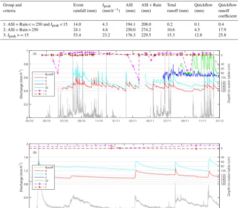
Figure 6.Time series of discharge (grey lines) and groundwater levels at sites 4, 5, 3, 32, 2 and 1; manually read sites are shown with dashed lines and diamonds at measurement points. Levels above zero at sites 1 and 2 occur as the soils are highly pugged in the riparian zone and water pooled on the surface in places, leading to slightly positive water levels being measured, at site 2 in particular.
ian zone during runoff events. Furthermore, the lower half of the riparian zone remained saturated to the surface for long periods during the runoff season. The data recorded at site 3 indicate that the water table at this site did not rise to the surface, even during events.
Looking at the discharge record in Fig. 6a, there were pe-riods where significant baseflow persisted between events. These correspond to periods where the water table at site 5 was above about 120 cm and at site 4 was above about 140 cm deep. Flow became more strongly persistent between rainfall events as the water table at sites 4 and 5 rose further. The water table recessions at sites 4 and 5 correspond to flow
re-cessions when the water table was above 120 and 140 cm at sites 4 and 5, respectively (Fig. 6b).
[image:13.612.61.530.86.496.2]Soil water storage (mm)
100 150 200 250 300
Depth to watertable (cm)
40
60
80
100
120
140
160
Site 5
Typical High intensity
Soil water storage (mm)
100 150 200 250 300
Depth to watertable (cm)
60
80
100
120
140
160
180
[image:14.612.97.235.68.333.2]Site 4
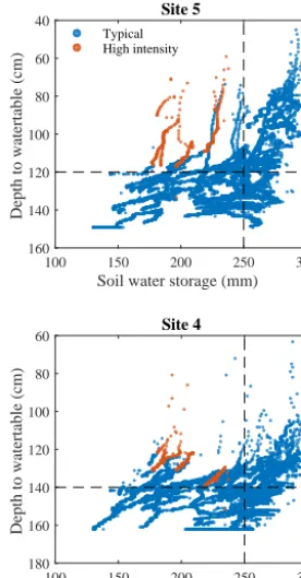
Figure 7.Soil water storage vs. water table level at sites 4 and 5. The red colour distinguishes events with high hourly rainfall
inten-sity, defined asIpeak> 15 mm, consistent with Fig. 5. The dashed
black lines correspond to values of water level and soil water stor-age discussed in the text. Soil water storstor-age is measured for the top 60 cm at the Automatic Weather Station.
chosen because they show significant dynamics and we had logged records available. Other sites with loggers had limited dynamics or short records. Site 5 in particular shows a rapid change in behaviour for soil water storage around 250 mm, which corresponds to the ASI+Rain threshold identified above. As soil water storage moves above this level, much higher water tables develop and those water tables showed relatively rapid recession when shallower than 120 cm. Sim-ilar observations were seen at site 4, but the corresponding depth was 140 cm. Figure 7 thus explains the linkage be-tween the 250 mm ASI+Rain threshold and runoff. When soil water storage exceeded this level, water tables rose and lateral subsurface drainage occurred, as evidenced by the re-cessions. The recessions in particular suggest that the water table moved into a more permeable zone on these occasions. This is consistent with soil profiles being characterised by mottled clay at depth, which is likely to have lower hydraulic conductivity. This behaviour at these two wells in combina-tion with the soil water and flow data indicate that the hill-slopes were becoming connected to the catchment outlet via subsurface flow from the hillslope to the riparian zone. Our analysis of isotope data below will add to the evidence for this. There were a few occasions where the water table re-sponded strongly for soil water storage of less than 250 mm
(Fig. 7). As indicated by the red colour, these corresponded to high intensity (Ipeak> 15 mm h−1) rainfall events.
Flow recessions provide information on the drainage char-acteristics of catchments. Figure 6 shows that the catchment flow usually ceased between events during the wet period, with no flow during dry periods. However, in August and early September 2010, continuous catchment flow endured for a month (Fig. 6). There was also a marked variation in the recession behaviour during August–September 2010 and at other times during the study period. To explore this, we cal-culated the recession constant,k(as inQ=Q0e−kt, where
Qtis discharge at timetduring the recession period,Q0is the
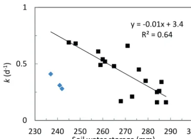
discharge at the beginning of the recession andkis the reces-sion constant). In fitting recesreces-sions, we target the period after the recession of the event flow, which typically ceased around 24 h after the end of the rainfall event. This was judged vi-sually by a marked change in slope of the recession hydro-graph plotted in semi-log space. Recessions were only fitted where a long enough period of reliable flow data (>=24 h) was available. Data availability was sometimes limited by the commencement of another event or flow falling to very low (< 0.05 mm h−1).kis plotted against soil water storage at the start of the catchment flow recession for individual events (Fig. 8). In total we could estimate values ofkfor 20 events. The three events in Fig. 8 coloured blue were from Novem-ber 2011 from a relatively dry period in late spring when there was a drying trend but where flow from the riparian area was just persisting. These were excluded from the fit-ting because, in our judgement, they appear to represent dif-ferent behaviour.kfor each event and the soil water storage at the start of the recession period were negatively correlated (R2=0.64) (Fig. 8). kdecreased as soil water storage in-creased at a rate of about 0.1 d−1 for each 10 mm increase
in soil water storage. Considering this and the transient na-ture of flow during dry periods, it is clear that the wetter the catchment is, the slower the recessions are. By inference, this suggests that greater (perhaps more spatially extensive) sub-surface connectivity is providing flows from the hillslope and maintaining catchment flow during wetter conditions. 3.3.2 Isotope and major ion results
y = -0.01x + 3.4 R² = 0.64
0 0.5 1
230 240 250 260 270 280 290 300
k
(d
-1)
[image:15.612.68.264.65.208.2]Soil water storage (mm)
Figure 8.Recession constant (k) and soil water storage at the start of the recession period for individual events. The choice of events is explained in the text, as are the three blue points.
Discharge (mm h
-1)
0 0.1 0.2 0.3 0.4 0.5 0.6 0.7 0.8 0.9 1
10/08/10 11/08/10 12/08/10 13/08/10 14/08/10
/
-80 -70 -60 -50 -40 -30 -20
Flow /D Rain /D Flow
10/08/10 11/08/10 12/08/10 13/08/10 14/08/10
0
2
4
6
Figure 9.Time series of total rainfall and discharge,2H of rainfall and runoff for the event on 12 August 2010.
these two events; therefore, these events were also excluded. For the event on 12 August 2010, the standard deviations were approximately 12 and 9 % for18O and2H, respectively, which we judged to be acceptable.
Figure 9 shows the event from 12 August 2010 during the wettest part of the study period. The antecedent soil water storage at the beginning of this event was 274 mm and to-tal rainfall was 17 mm. We used a pre-event low-flow sam-ple from ∼2 days before the analysed event as the pre-event end member. We estimated the contribution at the time of each stream water sample. Over the study period δ2H (δ18O) for rainfall varied between −7 and −83 ‰ (−1.4 and 12.6 ‰) and isotopic concentrations for low flows were highly damped. Low flow samples from the RBF flume be-fore and after the event showed a δ2H (δ18O) of −27 ‰ (−4.1 ‰) and rainfall for this event was strongly depleted (three samples prior to and during the event δ2H= −42, −67 and −57 ‰, δ18O= −6.5, −9.8 and −8.2 ‰), com-pared with low flow. The runoff samples showed a very
dif-ferent isotopic concentration during the rising limb and the peak of the hydrograph (δ2H= −43 ‰,δ18O= −6.8 ‰) in comparison to antecedent low flow. This shows that the iso-topic concentration moves significantly towards the rainfall sample concentrations. To estimate the overall event water contribution we first separated the hydrograph at each sam-pling time and then interpolated the fraction of event water between stream water sampling times and combined this with the discharge hydrograph to calculate the overall volume of event water. This analysis suggests that the percentage of rain becoming runoff based onδ2H andδ18O is 4.4 % (3.4–5.4 %) and 3.6 % (3.0–4.2 %), respectively. The figures in the brack-ets are 95 % confidence intervals for uncertainty based on the hydrograph separation uncertainty only. These results sug-gest that precipitation on the saturated area generates direct runoff in amounts that are close to what would be expected (i.e. 100 % runoff) given that the saturated area is around 5– 6 % of the catchment area.
Another interesting event is the higher intensity (Ipeak=15 mm h−1) event on 8 November 2011. Major
[image:15.612.47.287.268.440.2]ion geochemistry data were available for this event. Fig-ure 10a shows the typical relationship between discharge and chloride concentration, with samples from this event identified by red. Figure 10b shows the time series of chlo-ride concentration along with the hydrograph. The first and second chloride samples, respectively, plot above and within the typical scatter of data in Fig. 10a, while the remaining samples plot well below the typical variation in chloride con-centration with flow (Fig. 10a). Similar plots are shown for sodium, magnesium, calcium and potassium in Supplement Fig. S1. Sodium and magnesium show similar behaviour to chloride. Potassium also shows somewhat anomalous behaviour but with anomalously high concentrations. The relationship between discharge and K+ is also different to Cl−, Na+and Mg2+in that concentrations increase slightly as discharge increases to above about 0.2 mm mm−1, rather than decline. Calcium does not show anomalous behaviour.
Given the late spring timing of this event, the first sam-ple probably reflects some evapoconcentration of solutes in the riparian area. The flow shows a rapid peak in response to the main rainfall burst followed by a sustained relatively low flow and a recession over the second half of the day sugges-tive of subsurface flow. Up until the end of the first flow peak (i.e. 06:00), there had been 23.4 mm of rainfall and 1 mm of runoff. This runoff volume is 4.3 % of the rainfall volume, which is similar to the proportion of event water that became runoff for the 12 August 2010 event discussed above.
4 Discussion
4.1 Runoff mechanisms
iso-Discharge (mm h-1)
0 0.5 1 1.5 2
Chloride (mg L )
0 20 40 60 80 100 120 140
All samples 8 Nov 2011
Rainfall
(mm
h )
-1
0
5
10
15
Chloride (mg L )
0 20 40 60 80 100 120 140
08/11 00:00 08/11 06:00 08/11 12:00 08/11 18:00 09/11 00:00
Discharge
(mm
h
)
-1
0 0.5 1 1.5
Flow Chloride
-1 -1
(a) (b)
Figure 10. (a)Discharge vs. Cl−concentration for all events. The red colour identifies samples from the event on 8 November 2011.(b)Time
series of rainfall, runoff and Cl−concentration for the event on 8 November 2011.
tope and major ion geochemistry data provide further sup-porting evidence. The rainfall plus antecedent soil water threshold of 250 mm that needs to be exceeded for runoff in most circumstances shows that wetness dependent runoff processes are important, that is, either saturation excess or subsurface stormflow. Shallow groundwater data combined with field mapping of surface saturated areas show that com-plete profile saturation is limited to about 5 % of the catch-ment area and that this saturation is persistent, with only a small variation (see Table 1) over the winter–spring season but reducing over the dry summer–autumn period. The extent of the saturated area at the riparian zone varied seasonally and between events. Field observations of surface saturation extending to the flume and well hydrograph measurements of the water table at the surface showed that the saturated area was highly connected to the catchment outlet and sug-gest that it would be expected to produce saturation excess runoff. This surface connection disappeared during the dry summer season when the water level in all wells fell below the surface (see Fig. 6), so that the saturated area in the ripar-ian zone disappeared. The isotope results for 12 August 2010 enabled the event runoff to be separated into event water and pre-event water contributions. Four to five percent of the rain-fall volume on the catchment appeared in the event runoff, which corresponds well to the proportion of surface saturated area in the catchment (5.5 %, Table 1), supporting the identi-fication of significant saturation excess runoff from this part of the catchment, as observed elsewhere (McGlynn and Mc-Donnell, 2003; Penna et al., 2016).
While saturation excess runoff undoubtedly occurs, many of the event runoff coefficients were well in excess of 5 %, and they approach 100 % under very wet conditions (Fig. 5). The event on 12 August showed a substantial pre-event water contribution; logged shallow wells show that the water table did not reach the surface in the steeper areas of the catch-ment, even within the convergent drainage lines under very wet conditions (e.g. sites 5 and 7). The recession behaviour of
wells in the catchment suggests subsurface flow moves down the catchment under wet conditions and the recession con-stant analysis shows that this connection becomes stronger as the catchment wets beyond 250 mm of stored water. This is all consistent with a substantial contribution of subsurface flow to event runoff once the catchment is sufficiently wet to establish subsurface connection with the riparian area, as has been inferred in other studies (Buttle et al., 2004; Detty and McGuire, 2010; Hewlett and Hibbert, 1967; Jencso et al., 2009; Penna et al., 2011).
Perhaps more surprisingly there was a group of events that produced runoff under conditions of relatively low soil wa-ter storage (ASI+Rain < 250 mm) but high rainfall intensity. This suggests that an intensity dependent runoff process is being triggered when rainfall exceeds some threshold for suf-ficient time, in this case about 15 mm of rainfall in an hour. It is worth noting that the 15 mm h−1threshold will be depen-dent on the time step used in calculating the intensity. The choice of time step needs to consider the travel time from hillslope to stream as run-on infiltration processes occurring on the catchment surface will impact the connectivity to the stream. Thus the most appropriate time to use for averaging intensity would be the average travel time to the stream be-cause it is this time period which is available to infiltrate rain-fall that has become runoff at the point scale. Here the choice of hourly rainfall was pragmatic, as that was the recording time step of the AWS, but it is also likely that it reasonably approximates the flow times.
[image:16.612.128.466.66.222.2]Fur-thermore, for the high intensity event on 8 November 2011, the flow after the main peak had a surprisingly low concen-tration of chloride (the cluster of low concenconcen-tration red points in Fig. 10a), which may suggest that the higher intensity acti-vated either overland or preferential flow paths, limiting soil contact time and leading to this low concentration.
The hydrograph from the event on 8 November 11 (the event that exceeded both thresholds, Fig. 10) shows both a rapid and a delayed runoff response. The concentration of chloride was unusually low during the delayed runoff com-ponent compared with all other events (with major ion data available). This may suggest limited contact with the catch-ment soils which could occur if macropore flow was impor-tant, but this explanation is not definitive. Of the two events with peak hourly intensities around 15 mm h−1, one also ex-ceeded the wetness (ASI+Rain) threshold of 250 mm and the other had a very low runoff coefficient (only 3 %), and hence these two events are somewhat equivocal in terms of the importance of intensity. However, the two events with peak hourly rainfall intensities around 30 mm h−1both pro-duced rapid runoff responses without a significant delayed component (Fig. 4) and had runoff coefficients (12 and 68 %) well in excess of the surface saturated area (5 %) in the catch-ment, showing clear evidence of the role of rainfall intensity of 30 mm h−1. Unfortunately isotope and major ion data were not available for those events to attempt to determine whether surface or subsurface pathways are important. Overall there is clear evidence for intensity dependent runoff mechanisms, especially for the largest 30 mm h−1events.
In summary, the process evidence relating runoff be-haviour to catchment wetness thresholds, together with the data from shallow wells, suggests a catchment where sub-surface flow leads to a seasonally saturated riparian area that produces saturation excess runoff in immediate response to rainfall. This saturation excess is augmented by subsur-face stormflow when the catchment wetness (ASI+Rain) exceeds a 250 mm threshold. This subsurface flow exfiltrates in the riparian area. Volume considerations provide evidence that, for many of the monitored events, water must be com-ing from outside the riparian area. This area is only about 5 % of the catchment, but quickflow runoff coefficients very regu-larly exceed this, often (about 1/3 of runoff events) exceeded 20 %, and on occasion exceeded 50 %. The role of both sat-uration excess runoff and subsurface stormflow is corrobo-rated to some extend by isotopic data from one event where the hydrograph separation shows a volume of event water similar to the volume of rainfall on the saturated area and by the highly damped isotopic signal in the stream in general. When hourly rainfalls exceed a threshold of 15–30 mm h−1, an intensity dependent runoff process is activated that also contributes flow from the hillslope area outside the riparian zone. It is not clear whether this is a purely surface runoff process or not. One of the key contributions of this work is clear hydrometric evidence of the interplay of both wetness and intensity dependent runoff processes in the one
catch-ment. These responses include two wetness dependent pro-cesses, saturation excess runoff and subsurface stormflow, and an intensity dependent process for which we cannot dis-tinguish between surface and subsurface flow pathways with our data.
4.2 Thresholds and connectivity in runoff production
We identified two important thresholds in the catchment re-sponse. The first is a wetness threshold of ASI+Rain ex-ceeding 250 mm. Under these conditions the water table ap-proaches the surface in the riparian area and water tables rise on the hillslope into what is inferred from relatively rapid hillslope water table recessions to be a more transmissive part of the soil profile (within∼120–140 cm of the surface). Based on the volume of event runoff (Table 1), the lack of surface saturation on the hillslope and the behaviour of shal-low wells (Fig. 6), we infer that the hillslope becomes con-nected to the riparian zone under these conditions. The ex-istence of a large volume of pre-event water in the event on 12 August 2010 (Fig. 8) adds further corroboration to this. Similar catchment wetness thresholds for connectivity and runoff generation have been reported elsewhere (Detty and McGuire, 2010; Penna et al., 2011; Tromp-van Meerveld and McDonnell, 2006b). These have been expressed either in terms of rainfall depth, antecedent soil water storage con-ditions, or a combination of these. Similar to our results, in a study of a forested subcatchment with highly permeable soils and a small riparian area, Detty and McGuire (2010) found a relationship between a threshold of 316 mm for ASI+Rain and the start of the event streamflow response. They showed that the ASI+Rain threshold corresponded to a water table height threshold. Based on this, they suggested that subsur-face flow, transmissivity feedback and preferential flow from hillslope to stream could be used to explain runoff mecha-nisms in their catchment. They did not observe either Hor-tonian overland flow or saturation overland flow (SOF) even during the largest events.