Large watershed flood forecasting with high resolution distributed hydrological model

www.hydrol-earth-syst-sci.net/21/735/2017/ doi:10.5194/hess-21-735-2017

© Author(s) 2017. CC Attribution 3.0 License.

Large-watershed flood forecasting with high-resolution distributed

hydrological model

Yangbo Chen, Ji Li, Huanyu Wang, Jianming Qin, and Liming Dong

Department of Water Resources and Environment, Sun Yat-sen University, Guangzhou 510275, China Correspondence to:Yangbo Chen ([email protected])

Received: 17 September 2016 – Published in Hydrol. Earth Syst. Sci. Discuss.: 26 September 2016 Accepted: 7 January 2017 – Published: 3 February 2017

Abstract. A distributed hydrological model has been suc-cessfully used in small-watershed flood forecasting, but there are still challenges for the application in a large watershed, one of them being the model’s spatial resolution effect. To cope with this challenge, two efforts could be made; one is to improve the model’s computation efficiency in a large watershed, the other is implementing the model on a high-performance supercomputer. This study sets up a physically based distributed hydrological model for flood forecasting of the Liujiang River basin in south China. Terrain data digital elevation model (DEM), soil and land use are downloaded from the website freely, and the model structure with a high resolution of 200 m×200 m grid cell is set up. The initial model parameters are derived from the terrain property data, and then optimized by using the Particle Swarm Optimiza-tion (PSO) algorithm; the model is used to simulate 29 ob-served flood events. It has been found that by dividing the river channels into virtual channel sections and assuming the cross section shapes as trapezoid, the Liuxihe model largely increases computation efficiency while keeping good model performance, thus making it applicable in larger watersheds. This study also finds that parameter uncertainty exists for physically deriving model parameters, and parameter opti-mization could reduce this uncertainty, and is highly recom-mended. Computation time needed for running a distributed hydrological model increases exponentially at a power of 2, not linearly with the increasing of model spatial resolu-tion, and the 200 m×200 m model resolution is proposed for modeling the Liujiang River basin flood with the Liuxihe model in this study. To keep the model with an acceptable performance, minimum model spatial resolution is needed. The suggested threshold model spatial resolution for model-ing the Liujiang River basin flood is a 500 m×500 m grid

cell, but the model spatial resolution with a 200 m×200 m grid cell is recommended in this study to keep the model at a better performance.

1 Introduction

Development of distributed hydrological models in the past decades has provided the potential to improve the wa-tershed flood forecasting capability. One of the most impor-tant features of the distributed hydrological model is that it divides watershed terrain into grid cells, which are regarded to have the same meaning of a real watershed; i.e., the grid cells have their own terrain properties and precipitation. Hy-drological processes are calculated at both the grid cell scale and the watershed scale, and the parameters used to calcu-late hydrological processes are also different at different grid cells. This feature enables it to describe the inhomogene-ity of both the terrain property and precipitation over water-shed. The distributed feature of the distributed hydrological model is a very important feature compared to the lumped model, which could help it better simulate the watershed hy-drological processes at all scales, small or large. The inho-mogeneity of precipitation over a watershed could also be well described in the model, this is very helpful in modeling large-watershed hydrological processes, particularly in trop-ical and sub-troptrop-ical regions where the flooding is driven by heavy storms. For this reason, the distributed hydrological model is usually regarded as having the potential to better simulate or forecast the watershed flood (Ambroise et al., 1996; Chen et al., 2016). Employing a distributed hydrolog-ical model for watershed food forecasting has been the new trend (Vieux et al., 2004; Chen et al., 2016; Cattoën et al., 2016; Witold et al., 2016; Kauffeldt et al., 2016).

The blueprint of a distributed hydrological model is re-garded to be proposed by Freeze and Harlan (1969); the first distributed hydrological model was the SHE model pro-posed by Abbott et al. (1986a, b). The distributed hydro-logical model requires different terrain property data for ev-ery grid cells to set up the model structure; therefore, it is data-driven model. In the early stage of distributed hydro-logical modeling, this posted great challenge for the appli-cation of distributed hydrological model, as the data were not widely available and inexpensively accessible. With the development of remote sensing sensors and techniques, ter-rain data covering global range with high resolution has be-come readily available and could be acquired inexpensively. For example, the digital elevation model (DEM) at 30 m grid cell resolution with global coverage could be freely downloaded (Falorni et al., 2005; Sharma and Tiwari, 2014), which largely enhances the development and application of the distributed hydrological models. After that, many dis-tributed hydrological models have been proposed, such as the WATERFLOOD model (Kouwen, 1988), THALES model (Grayson et al., 1992), VIC model (Liang et al., 1994), DHSVM model (Wigmosta et al., 1994), CASC2D model (Julien et al., 1995), WetSpa model (Wang et al., 1997), GBHM model (Yang et al., 1997), WEP-L model (Jia et al., 2001), Vflo model (Vieux et al., 2002), tRIBS model (Vivoni et al., 2004), WEHY model (Kavvas et al., 2004), Liuxihe model (Chen et al., 2011, 2016), etc.

uses complex equations with physical meanings to calculate the hydrological processes; therefore, it needs much more computation resources than that of lumped model, and the re-quired computation resources increase exponentially with the increase of the model spatial resolution. Therefore, in mod-eling flood processes of a large watershed, the computation time needed for running the distributed hydrological model would be huge if the model spatial resolution is kept high, which may make the model application impractical due to the high running cost. So if a distributed hydrological model needs to be applied in a large watershed, a coarser resolu-tion is the only choice, and the model’s capability will be impacted with less satisfactory results. This is also called the scaling effect of a distributed hydrological modeling. For this reason, current application for watershed flood forecasting is either limited to a small watershed with higher resolution or a coarser resolution in a large watershed, i.e., a trade-off be-tween the model performance and running cost.

Presently forecasting large-watershed flooding has been in great demand as it impacts people and their properties at large range, but, due to the scale effect, current distributed hydrological models employed for a large watershed are at coarser resolution, which lowers its capability for flood forecasting and warning. For example, past application of a distributed hydrological model for large-watershed flood forecasting is at a resolution coarser than 1 km grid cell (Lohmann et al., 1998; Vieux et al., 2004; Stisen et al., 2008; Rwetabula et al., 2007); the models employed in the pan-European Flood Awareness System (EFAS; Bartholmes et al., 2009; Thielen et al., 2009, 2010; Sood and Smakhtin, 2015; Kauffeldt et al., 2016) are at 1–10 km grid cell, which makes the result only applicable for flood warning.

The challenge for distributed hydrological model applica-tion in large-watershed flood forecasting is its need for huge computational resources; to cope with this challenge, two forts could be made. One is to improve the computation ef-ficiency of distributed hydrological modeling in a large wa-tershed, and the other is implementing the model on a high-performance supercomputer; therefore, if the users are will-ing to pay a high computation cost, the flood forecastwill-ing of a large watershed with high resolution could be done. In this study, the Liuxihe model (Chen et al., 2011, 2016), a physi-cally based distributed hydrological model proposed for wa-tershed flood forecasting, has been used for flood forecasting of a large watershed in southern China to validate the fea-sibility of a distributed hydrological model’s application for large-watershed flood forecasting.

2 Method and data 2.1 Liujiang River basin

The river basin studied in this paper is the Liujiang River basin (herein after referred to as LRB) in south China, which

is the first-order tributary of the Pearl River. LRB origi-nates from the village Lang in Guizhou Province, and drains though the Guizhou Province, Guangxi Zhuang Autonomous Region and Hunan Province with 72 % of its drainage area in the Guangxi Zhuang Autonomous Region. The length of its main channel is 1121 km, and the total drainage area is 58 270 km2, which makes it a large river basin in China.

LRB is a mountainous watershed. There are high moun-tains in the north and northwest of the watershed with high elevation, whereas in the south and southeast areas, the ele-vations are relatively low. This topography helps form severe flooding in the middle and downstream. The basin is in the sub-tropical monsoon climate zone with an average annual precipitation of 1800 mm, and the precipitation distribution is highly uneven both at spatial and temporal scale with 80 % of its annual precipitation occurring in the summer. LRB is in the center of storm zone of the Zhuang Autonomous Re-gion; heavy storm was very frequent in the past. There have been 59 disastrous flooding events in the past 400 years with recording since 1488, which makes the LRB the tributary with the most disastrous flooding among all the first-order tributaries of the Pearl River. In the watershed, there are no significant reservoirs to store flood runoff; therefore, flood forecasting is one of the most effective ways of flood man-agement.

2.2 Liuxihe model

The Liuxihe model is a physically based distributed hydro-logical model proposed mainly for watershed flood forecast-ing (Chen, 2009; Chen et al., 2011, 2016). Like other dis-tributed hydrological models, the Liuxihe model divides the watershed into grid cells based on the DEM of the stud-ied watershed. To keep a reasonable model performance, in past experiences of Liuxihe model research and appli-cation, the model resolution is limited to 90 m×90 m or 100 m×100 m, but only used in small watersheds (Chen, 2009; Chen et al., 2011, 2013, 2016; Liao et al., 2012a, b; Xu et al., 2012a, b). Precipitation, evaporation and runoff production are calculated at cell scale; i.e., runoff routes first on the cell, then along the cell to river channel and finally to the watershed outlet. As the Liuxihe model is mainly used in sub-tropical regions, the runoff production is calculated based on the saturation-excess mechanism (Zhao, 1977). The runoff routing is classified as hillslope routing, river chan-nel routing, subsurface routing and underground routing. The hillslope routing is regarded as a one-dimensional unsteady flow, and the kinematical wave approximation is employed to do the routing. The river channel routing is also regarded as a one-dimensional unsteady flow, but the diffusive wave ap-proximation is employed to do the routing. The above meth-ods are widely used in the dominant distributed hydrological models.

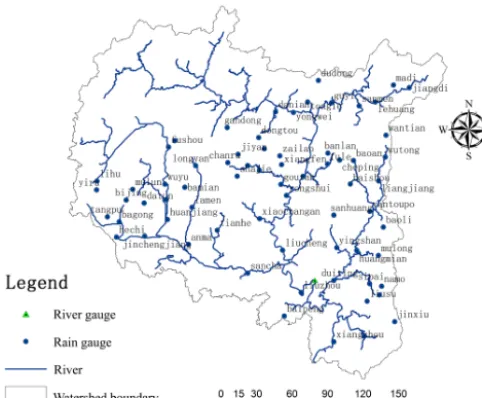
Figure 1.Sketch map of the Liujiang River basin (LRB).

assumption, the river channel size could be represented with three dimensions, including the bottom width, side slope and bottom slope. One of the advantages with this assumption is that the river channel cross section size could be estimated with remotely sensed data (Chen et al., 2011); therefore, the Liuxihe model could do river channel runoff routing physi-cally, thus making the Liuxihe model a fully distributed hy-drological model. As there are too many river channel cross sections, and many of them are in the upstream of the water-shed where they are not easily accessed, in real hydrological modeling, directly measuring the river channel cross section sizes is impractical considering the high cost. For this rea-son, most of the distributed hydrological models could not be applied in real applications or simply routed in the runoff with lumped methods, which makes the model not a fully distributed hydrological model, thus lowering the model’s capability in simulating or forecasting the watershed flood processes. Another advantage of this assumption is that it also simplifies the runoff routing, thus improving the model’s computation efficiency. For this reason, even though the Li-uxihe model has a very high resolution, it still could be used in real-time flood forecasting. This feature of the Liuxihe model in estimating river channel cross section sizes gives it the potential to be used in large-watershed flood forecast-ing.

Like other distributed hydrological models, when used in ungauged or data-poor watershed flood forecasting, the Liux-ihe model derives model parameters physically from the ter-rain property data. But if there is observed hydrological data, automatic parameter optimization methods could been tried. But an automatic parameter optimization needs thousands of model runs, which makes it difficult to be used widely due to huge computing source requirement, and also means it takes a long time to set up the model. For this reason, a

pub-lic computer cloud was set up for optimizing the parameters of the Liuxihe model, which employs parallel computation techniques and was implemented on a supercomputer sys-tem (Chen et al., 2013). With this development, the Liuxihe model could easily optimize its model parameters.

Above advancements of the Liuxihe model in estimat-ing river channel cross section sizes with remotely sensed data, automatic parameters optimization and supercomput-ing gives it the potential to be used in large-watershed flood forecasting; therefore, in this study the Liuxihe model is em-ployed to study flood forecasting in the LRB.

2.3 Hydrological data

There are 66 rain gauges installed in the watershed. In this study, hydrological data of 30 flood events have been col-lected, including the precipitation of the rain gauges and the river discharge of the Liuzhou river gauge, which is located in the downstream of the watershed and is close to the outlet, as shown in Fig. 1, with a hourly step; brief information on these flood events is listed in Table 1.

2.4 Terrain property data

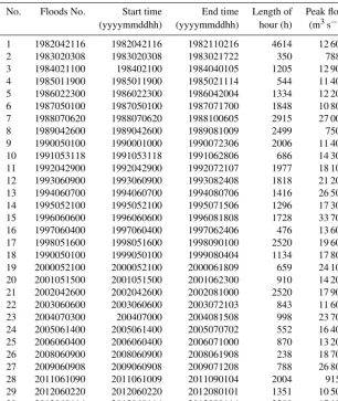
Terrain property data include a DEM, land use/cover map and soil map, which are used for setting up the distributed hydrological model for flood forecasting. In this study, the DEM was downloaded from the SRTM database (Falorni et al., 2005; Sharma and Tiwari, 2014), the land use type was downloaded from the USGS land use type database (Love-land et al., 1991, 2000), and the soil type was downloaded from FAO soil type database (http://www.isric.org). The downloaded DEM has a spatial resolution of 90 m×90 m, considering LRB is large. The running load for the model with a resolution of 90 m×90 m may be too heavy to run in this study; therefore, the DEM is rescaled to the resolutions of 200 m×200 m, as shown in Fig. 2a. The downloaded land use and soil type were at a resolution of 1000 m×1000 m, and therefore are rescaled to the same resolution as the DEM, as shown in Fig. 2b and c, respectively.

The highest elevation and the lowest elevation of the LRB are 2124 and 42 m, respectively. There are nine land use types, including evergreen needle leaved forest (18.1 %), evergreen broadleaved forest (31.0 %), shrubbery (32.5 %), mountain and alpine meadow (0.1 %), slope grass-land (13.7 %), urban area (0.1 %), river (0.2 %), lakes (0.3 %) and cultivated land (4 %).

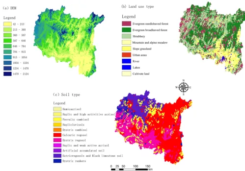
Table 1.Brief information of flood events in LRB.

No. Floods No. Start time End time Length of Peak flow (yyyymmddhh) (yyyymmddhh) hour (h) (m3s−1) 1 1982042116 1982042116 1982110216 4614 12 600 2 1983020308 1983020308 1983021722 350 7880 3 1984021100 198402100 1984040105 1205 12 900 4 1985011900 1985011900 1985021114 544 11 400 5 1986022300 1986022300 1986042004 1334 12 200 6 1987050100 1987050100 1987071700 1848 10 800 7 1988070620 1988070620 1988100605 2915 27 000 8 1989042600 1989042600 1989081009 2499 7500 9 1990050100 1990001000 1990072306 2006 11 400 10 1991053118 1991053118 1991062806 686 14 300 11 1992042900 1992042900 1992072107 1977 18 100 12 1993060900 1993060900 1993082408 1818 21 200 13 1994060700 1994060700 1994080706 1416 26 500 14 1995052100 1995052100 1995071506 1296 17 300 15 1996060600 1996060600 1996081808 1728 33 700 16 1997060400 1997060400 1997062406 476 13 600 17 1998051600 1998051600 1998090100 2520 19 600 18 1990050100 1999050100 1999080404 1134 17 800 19 2000052100 2000052100 2000061809 659 24 100 20 2001051500 2001051500 2001062300 910 14 200 21 2002042600 2002042600 2002081000 2520 17 900 22 2003060600 2003060600 2003072103 843 11 600 23 2004070300 200407000 2004081508 998 23 700 24 2005061400 2005061400 2005070702 552 16 400 25 2006060400 2006060400 2006071000 870 13 200 26 2008060900 2008060900 2008061908 238 18 700 27 2009060908 2009060908 2009071208 788 26 800 28 2011061090 2011061009 2011090104 2004 9153 29 2012060220 2012060220 2012080101 1351 10 500 30 2013060114 2013060114 2013090114 2200 17 100

3 Results

3.1 Liuxihe model setup

Considering that the LRB is large, the DEM with a 200 m×200 m resolution is adopted to set up the model structure, not the original 90 m×90 m resolution. The whole watershed is first divided into 1 469 900 cells by the DEM horizontally, which were further categorized into hillslope cells and river cells. By using Strahler method (Strahler, 1957), the river channel is divided into a three-order sys-tem as shown in Fig. 3, which divides all of the cells into 1 463 204 hillslope cells and 6696 river cells.

To estimate the river channel sizes, 178 virtual nodes were set on the river channel system, and 225 virtual channel sec-tions were formed as shown in Fig. 3. As in the Liuxihe model, the shape of the virtual channel sections is assumed to be trapezoid, and therefore the cross section size is rep-resented by three dimensions, including bottom width, side slope and bottom slope. As proposed in Liuxihe model, the bottom width is estimated based on the satellite remote

sens-ing imageries. For the side slope, it is a low-sensitive data and could be estimated based on local experiences. For the bottom slope, it is calculated with the DEM along the virtual channel section.

3.2 Parameter optimization

Figure 2.Terrain properties of LRB.

Figure 3.Liuxihe model structure setup for LRB (200 m×200 m resolution).

For the soil-related parameters include the water content at saturation condition, the water content at field condition, the water content at wilting condition, hydraulic conductivity

Table 2.The initial values of land use/cover-related parameters.

Land use/cover evaporation roughness coefficient coefficient Evergreen needle leaf forest 0.7 0.4 Evergreen broadleaf forest 0.7 0.6

Shrubbery 0.7 0.4

Mountains and alpine meadow 0.7 0.2 Slope grassland 0.7 0.3

City 0.7 0.05

Cultivated land 0.7 0.35

conduc-Table 3.The initial values of soil-related parameters.

Soil type Soil Water content Water content Hydraulic conductivity thickness at saturation at field at saturation condition (mm) condition condition (mm h−1)

Humic Acrisol 800 0.65 0.32 3.5

Haplic and high-active Acrisol 900 0.57 0.43 4.2 Ferralic cambisol 850 0.63 0.38 20.5

Haplic Luvisols 980 0.46 0.15 2.6

Dystric cambisol 950 0.55 0.41 14

Calcaric Regosol 1100 0.62 0.24 5.6 Dystric regosol 840 0.45 0.27 12.5 Haplic and weak active Acrisol 1050 0.58 0.16 4.6 Artificial accumulated soil 1000 0.63 0.34 5.5 Eutric Regosol and black limestone 550 0.75 0.27 3.5

Dystric rankers 380 0.78 0.36 8

tivity at saturation condition are estimated by using the Soil Water Characteristics Hydraulic Properties Calculator (Arya et al., 1981) based on soil texture, organic matter, gravel con-tent, salinity and compaction. The estimated initial values of soil-related parameters are listed in Table 3.

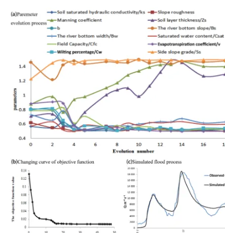
In this study, the PSO algorithm is employed to optimize the initial model parameters, as the PSO algorithm has been integrated into the Liuxihe model cloud (Chen et al., 2013, 2016). The number of particles of the PSO algorithm is set to 20, while the value range of inertia weightωis set to 0.1 to 0.9, the value range of acceleration coefficients C1 is set to 1.25 to 2.75, and C2 to 0.5 to 2.5, and the maximum iter-ation is set to 50. The flood event of 20080609 (see Fig. 4) is selected to optimize the parameters of the Liuxihe model, and Fig. 4 shows the result of the parameter optimization. Among them, Fig. 4a is the parameters evolving process, Fig. 4b is the changing curve of objective function, which is set to minimize the peak flow error, and Fig. 4c is the sim-ulated hydrograph of flood event 20080609 (see Fig. 4) with the optimized parameters.

From the results in Fig. 4, it could be found that after 12 evolutions, the parameters optimization process converges to its optimal values, and the optimal parameters are achieved, the simulated hydrological process of a flood event that is used for parameter optimization is quite a good fit to the ob-served hydrological process and it could be said that the pa-rameter has a good optimization effect.

As mentioned above, the automatic parameter optimiza-tion of the distributed hydrological model is very time con-suming. In this study, even a supercomputer is employed with parallel computational techniques, and the time used for this parameter optimization is overwhelming; the total time used for achieving the above optimal parameters of the Liuxihe model for LRB flood forecasting is 220 h, more than 9 days. Considering several runs are usually needed before achieving the final results, the parameter optimization procedure may

Figure 4.Parameter optimization results of Liuxihe model for LRB with PSO algorithm.

take a few months, but this run time is really a good invest-ment and the validation results proves this is worth doing. 3.3 Model validation

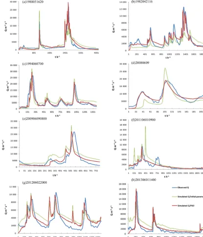
The other 29 flood events were simulated by using the Liux-ihe model with the above optimized parameters, and the sim-ulated hydrographs of eight flood events are shown in Fig. 5, the simulated hydrographs of eight flood events with initial parameters are also shown in Fig. 5.

Figure 5.Simulated flood events by Liuxihe model with optimized parameters.

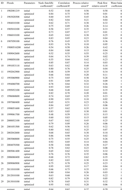
well, particularly the simulated peak flow is quite good, and the simulated hydrological processes with optimized model parameters improved the simulated hydrological processes largely. To further analyze the effect of parameter optimiza-tion on model performance improvement, five evaluaoptimiza-tion in-dices of the simulated flood events, including the Nash– Sutcliffe coefficient, the correlation coefficient, the process relative error, the peak flow error and water balance coeffi-cient are calculated from the simulated results. Table 4 listed

the five indices for both the simulated results with the initial parameters and the optimized parameters.

sim-Table 4.Evaluation indices of the simulated flood events.

ID Floods Parameters Nash–Sutcliffe Correlation Process relative Peak flow Water balance coefficient/C coefficient/R error/P relative error/E coefficient/W

1 1982081219 initial 0.52 0.48 0.56 0.58 0.52

optimized 0.84 0.75 0.30 0.01 0.83

2 1983020308 initial 0.60 0.55 0.45 0.26 0.65

optimized 0.82 0.84 0.21 0.04 0.89

3 1984010100 initial 0.62 0.71 0.38 0.32 0.75

optimized 0.75 0.89 0.26 0.14 0.96

4 1985010100 initial 0.58 0.57 0.35 0.33 0.85

optimized 0.73 0.87 0.17 0.01 1.05

5 1986010100 initial 0.65 0.62 0.38 0.25 0.62

optimized 0.83 0.85 0.23 0.04 0.94

6 1987050100 initial 0.76 0.45 0.35 0.36 0.58

optimized 0.93 0.76 0.10 0.05 1.01

7 19880516200 initial 0.54 0.58 0.26 0.42 0.82

optimized 0.84 0.80 0.15 0.04 0.90

8 1989042600 initial 0.52 0.55 0.55 0.25 0.62

optimized 0.64 0.74 0.39 0.02 0.88

9 1990050100 initial 0.55 0.64 0.42 0.23 0.55

optimized 0.85 0.87 0.14 0.03 0.85

10 1991053118 initial 0.63 0.62 0.40 0.18 0.68

optimized 0.80 0.76 0.25 0.04 0.95

11 1992042900 initial 0.48 0.59 0.35 0.34 0.65

optimized 0.66 0.84 0.20 0.11 0.89

12 1993060900 initial 0.75 0.65 0.38 0.28 0.84

optimized 0.91 0.89 0.24 0.09 1.05

13 1994060700 initial 0.78 0.64 0.32 0.26 1.25

optimized 0.93 0.85 0.14 0.04 0.85

14 1995052100 initial 0.68 0.48 0.42 0.35 0.65

optimized 0.82 0.70 0.20 0.01 0.81

15 1996060600 initial 0.74 0.65 0.25 0.23 0.54

optimized 0.90 0.93 0.18 0.02 0.86

16 1997060400 initial 0.65 0.51 0.23 0.26 0.65

optimized 0.84 0.87 0.13 0.06 0.95

17 1998051600 initial 0.57 0.62 0.35 0.18 0.68

optimized 0.83 0.85 0.30 0.01 1.05

18 1999061700 initial 0.48 0.59 0.33 0.15 0.55

optimized 0.60 0.83 0.15 0.05 0.80

19 2000052100 initial 0.67 0.62 0.45 0.25 0.58

optimized 0.79 0.89 0.26 0.06 0.83

20 2001051500 initial 0.62 0.56 0.32 0.22 0.68

optimized 0.80 0.82 0.25 0.07 0.82

21 2002042600 initial 0.68 0.65 0.38 0.18 0.57

optimized 0.86 0.90 0.24 0.02 0.87

22 2003060600 initial 0.75 0.55 0.25 0.26 0.55

optimized 0.92 0.85 0.14 0.04 0.76

23 2004070300 initial 0.58 0.68 0.38 0.27 0.68

optimized 0.78 0.82 0.23 0.08 0.85

24 2005061400 initial 0.65 0.62 0.52 0.32 0.65

optimized 0.76 0.76 0.35 0.06 0.74

25 2006060400 initial 0.68 0.72 0.62 0.35 0.53

optimized 0.82 0.83 0.30 0.10 0.86

26 2009060908 initial 0.75 0.78 0.25 0.23 1.22

optimized 0.95 0.92 0.17 0.04 0.09

27 2011010100 initial 0.66 0.75 0.35 0.55 1.66

optimized 0.80 0.84 0.26 0.03 1.02

28 2012010100 initial 0.63 0.68 0.34 0.22 1.42

optimized 0.82 0.79 0.20 0.05 0.80

29 2013010100 initial 0.78 0.65 0.31 0.32 1.35

optimized 0.95 0.82 0.20 0.06 0.92

average initial 0.64 0.62 0.37 0.29 0.78

Table 5.Grid cell numbers with different model spatial resolution.

Model resolution Number of Number of Number of grid cells hillslope cells river cells 200 m×200 m 1 469 900 1 463 204 6696 400 m×400 m 367 475 365 801 1674 500 m×500 m 235 184 234 113 1071 600 m×600 m 163 322 162 578 744 1000 m×1000 m 58 796 58 528 268

ulated hydrological processes with the optimized model pa-rameters are also good improvements to those simulated with the initial parameters, which are 0.64, 0.62, 0.37, 0.29 and 0.78. They are excellent in improving in all five indices, with the average increases of 0.18, 0.21 and 0.09 of the average Nash–Sutcliffe coefficient, correlation coefficient and water balance coefficient, respectively, and the average decreases of the peak flow error and process relative error are 24 % and 15 %, respectively. Therefore, it could be concluded that the Liuxihe model setup in LRB with optimized parame-ters is reasonable and could be used for flood forecasting of LRB. This also implies that the parameter optimization of the distributed hydrological model could improve model perfor-mances, and it should be done when it is possible.

4 Discussions

4.1 Computation time vs. model resolution

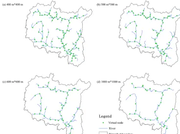
To evaluate the spatial resolution scaling effect of distributed hydrological modeling in LRB, the DEM with a 90 m×90 m resolution is rescaled to the resolutions of 400 m×400 m, 500 m×500 m, 600 m×600 m and 1000 m×1000 m; the land use and soil type at a 1000 m×1000 m resolution are also rescaled to the same resolutions of the DEM used. Li-uxihe models for LRB flood forecasting at the above resolu-tions are then set up with the above methods, and the model structures are shown in Fig. 6.

With different spatial resolutions, the numbers of grid cells, hillslope cells and river cells are different, but the river channel orders are all set to 3, the numbers of vir-tual channel nodes for the 400 m×400 m, 500 m×500 m, 600 m×600 m and 1000 m×1000 m resolution models are 100, 68, 46 and 33, respectively, and numbers of grid cells, hillslope cells and river cells with different model resolution are listed in Table 5. The sizes of every virtual cross sections in Fig. 6 are measured with the in Fig. 6.

From Table 5, it could be seen, number of grid cells of the model with a 200 m×200 m resolution is 4 times that of the 400 m×400 m resolution, 6.25 times that of the 500 m×500 m resolution, 9 times that of the 600 m×600 m resolution, and 25 times that of the 1000 m×1000 m

Figure 6.Liuxihe model structure setup for LRB with different resolution.

tion; it increases at an approximate exponential of power 2, not linearly with the model resolution.

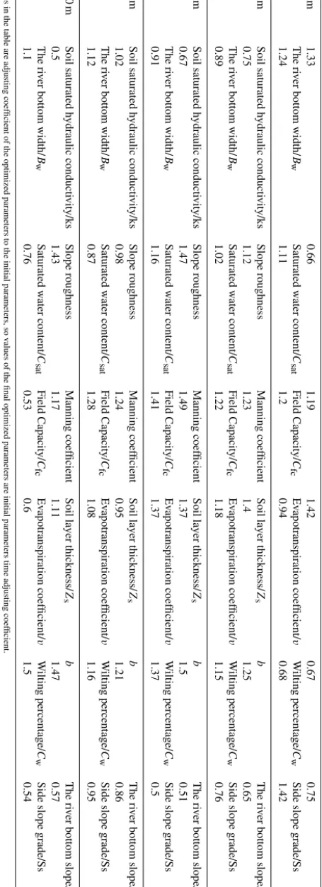
Parameters of the models with 400 m×400 m, 500 m×

500 m, 600 m×600 m and 1000 m×1000 m resolutions are optimized with the PSO algorithm by using the same flood event data, and listed in Table 6. From the results it could be seen that some parameters are significantly different with resolution variation, but some change little, and this implies that the model parameters are resolution dependent.

Computation times required for parameter optimization are quite different. For the model with a 200 m×200 m reso-lution, the time for parameter optimization is 220 h, whereas that for models with 400 m×400 m, 500 m×500 m, 600 m×600 m and 1000 m×1000 m the resolutions are 80, 55, 35 and 12 h, respectively. The times needed for param-eter optimization of the model at 200 m×200 m resolution is 2.75 times that for the 400 m×400 m resolution model, 4 times that for the 500 m×500 m resolution model, 6.3 times that for the 600 m×600 m resolution model, and 18.3 times that for the 1000 m×1000 m resolution model. Considering the time needed for model run, the 200 m×200 m model res-olution is regarded as appropriate for LRB.

4.2 Model performance vs. model resolution

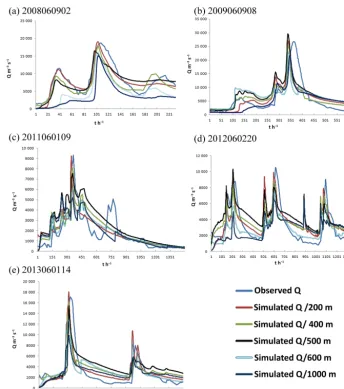
The other 29 flood events are also simulated with the mod-els at 400 m×400 m resolution, 500 m×500 m resolution, 600 m×600 m resolution and 1000 m×1000 m resolution.

Simulated hydrograph of five flood events, including two big,two medium and one small, are shown in Fig. 7.

Figure 7.Simulated results with different model resolutions.

also much closer to the observation; it is a good simulation result and could be recommended for flood forecasting of the LRB. As the results are good enough, there is no need to fur-ther explore the finer model resolution.

5 Conclusions

By employing Liuxihe model, a physically based distributed hydrological model, this study sets up a distributed hydro-logical model for the flood forecasting of the Liujiang River basin in southern China that could be regarded as a large wa-tershed. Terrain data including DEM, soil type and land use type are downloaded from the website freely, and the model structure with a high resolution of 200 m×200 m grid cell is set up, which divides the whole watershed into 1 469 900 grid cells that is further divided into 1 463 204 hillslope cells and 6696 river cells. The initial model parameters are derived from the terrain property data, and then optimized by

us-ing the PSO algorithm with one observed flood event, which improves the model performance largely. 29 observed flood events are simulated by using the model with optimized pa-rameters, the results are analyzed, and the model scaling ef-fects are studied. Based on these studies, following conclu-sions are suggested.

this method has a reasonable performance; i.e., this sim-plification has not sacrificed the model’s flood simula-tion accuracy significantly, and therefore this simplifi-cation could be used in large-watershed-distributed hy-drological modeling, including the Liuxihe model and other models.

2. Uncertainty exists for physically derived model param-eters. Parameter optimization could reduce parameter uncertainty, and is highly recommended to do so when there is some observed hydrological data. In this study, the simulated hydrograph with optimized model param-eters fits the observed hydrograph more in shape than that simulated with initial model parameters, and the five evaluation indices are improved also. The average increases of the Nash–Sutcliffe coefficient, correlation coefficient and water balance coefficient are 0.18, 0.21 and 0.09, respectively, and the average decreases of the peak flow error and process relative error are 24 and 15 %, respectively; this implies that the model perfor-mance is improved significantly with parameter opti-mization.

3. Computation time needed for running a distributed hy-drological model increases exponentially at an approx-imate power of 2, not linearly with the increasing of model spatial resolution. In this study, the computa-tion time required for parameter optimizacomputa-tion for the model with a 200 m×200 m resolution is 220 h, that is 4 times of that of the model at 500 m×500 m and 18.3 times of that of the model at 1000 m×1000 m res-olution. Based on the Liuxihe model cloud system im-plemented on the high-performance supercomputer, the 200 m×200 m model resolution is the highest resolu-tion that could be fulfilled in modeling Liujiang River basin flooding with the Liuxihe model, considering the computation cost. This also means that if the user could pay the high computation cost, then a larger watershed could also be modeled with the Liuxihe model by im-plemented the Liuxihe model cloud system on a much more advanced high-performance supercomputer, this could be easily done presently if the user thinks this in-vestment is a worth doing.

4. In forecasting a watershed flood by using the distributed hydrological model, minimum model spatial resolution needs to be maintained to keeping the model at an ac-ceptable performance. Usually if the model’s spatial resolution increases, i.e., the grid cell gets smaller, the model performance is better, but this will increase the run time significantly; therefore, there is a threshold model spatial resolution to keep the model performance reasonable while keeping the model run at the least amount of time. In this study, the threshold model spa-tial resolution is at 500 m×500 m grid cell, but the res-olution at 200 m×200 m grid cell is recommended by

trading-off between the computation cost and the model performance. This conclusion may be different in differ-ent watersheds for the Liuxihe model, or even differdiffer-ent in the same watershed for different models.

5. Terrain data downloaded freely from the website de-rived a river channel system that is very similar to the natural river channel system after it is rescaled from its original spatial resolution of 90 m×90 m to 200 m×200 m, 500 m×500 m and 1000 m×1000 m, but the higher-resolution DEM describes the river chan-nel more in details. This means that the freely down-loaded DEM could be used to set up the Liuxihe model for Liujiang River basin flood forecasting.

6 Data availability

The DEM data were downloaded from the SRTM database (http://srtm.csi.cgiar.org), the land use type data were down-loaded from the USGS Global Land Cover Characteriza-tion (GLCC) database (https://lta.cr.usgs.gov/GLCC), and the soil type data were downloaded from FAO soil type database (http://www.isric.org). The flood event data includ-ing the rainfall and river discharge data are provided by the Bureau of Hydrology, Pearl River Water Resources Commis-sion, China; this data can only be used for this study and can-not be provided to others by the authors.

Competing interests. The authors declare that they have no conflict

of interest.

Acknowledgements. This study is supported by the Special

Research Grant for the Water Resources Industry (funding no. 201301070), the National Science Foundation of China (fund-ing no. 50479033), and the Basic Research Grant for Universities of the Ministry of Education of China (funding no. 13lgjc01). Edited by: Q. Chen

Reviewed by: two anonymous referees

References

Abbott, M. B., Bathurst, J. C., Cunge, J. A., O’Connell, P. E., and Rasmussen, J.: An Introduction to the European Hydrologic System-System Hydrologue Europeen, “SHE”, a: History and Philosophy of a Physically-based, Distributed Modelling Sys-tem, J. Hydrol., 87, 45–59, 1986a.

Ambroise, B., Beven, K., and Freer, J.: Toward a generalization of the TOPMODEL concepts: Topographic indices of hydrologic similarity, Water Resour. Res., 32, 2135–2145, 1996.

Anderson, A. N., McBratney, A. B., and FitzPatric, K. E.: A soil mass, surface and spectral fractal dimensions estimated from thin section photographs, Soil Sci. Soc. Am. J., 60, 962–969, 1996. Arya, L. M. and Paris, J. F.: A physioempirical model to predict

the soil moisture characteristic from particle-size distribution and bulk density data, Soil Sci. Soc. Am. J., 45, 1023–1030, 1981. Bartholmes, J. C., Thielen, J., Ramos, M. H., and Gentilini, S.: The

european flood alert system EFAS – Part 2: Statistical skill as-sessment of probabilistic and deterministic operational forecasts, Hydrol. Earth Syst. Sci., 13, 141–153, doi:10.5194/hess-13-141-2009, 2009.

Burnash, R. J. C.: The NWS river forecast system-catchment mod-eling, Computer models of watershed hydrology, edited by: Singh, V. P., Water Resource Publications, Littleton, Colorado, 311–366, 1995.

Cattoën, C., McMillan, H., and Moore, S.: Coupling a high-resolution weather model with a hydrological model for flood forecasting in New Zealand, J. Hydrol., 55, 1–23, 2016. Chen, H. and Mao, S.: Calculation and Verification of an

Univer-sal Water Surface Evaporation Coefficient Formula, Advances in Water Science, 6, 116–120, 1995.

Chen, X.: Analysis on flood disasters in China, Marine Geology and Quaternary Geology, 15, 161–168, 1995.

Chen, Y.: Liuxihe Model, China Science and Technology Press, September 2009.

Chen, Y., Ren, Q. W., Huang, F. H., Xu, H. J., and Cluckie, I.: Liux-ihe Model and its modeling to river basin flood, J. Hydrol. Eng., 16, 33–50, 2011.

Chen, Y., Dong, Y., and Zhang, P.: Study on the method of flood forecasting of small and medium sized catchment, proceeding of the 2013 annual meeting of the Chinese Society of Hydraulic Engineering, 1001–1008, 2013.

Chen, Y., Li, J., and Xu, H.: Improving flood forecasting capa-bility of physically based distributed hydrological models by parameter optimization, Hydrol. Earth Syst. Sci., 20, 375–392, doi:10.5194/hess-20-375-2016, 2016.

EEA: Mapping the Impacts of Natural Hazards and Technologi-cal Accidents in Europe: an Overview of the Last Decade, EEA Technical Report, European Environment Agency, Copenhagen, doi:10.2800/62638, p. 144, 2010.

Falorni, G., Teles, V., Vivoni, E. R., Bras, R. L., and Ama-ratunga, K. S.: Analysis and characterization of the vertical accuracy of digital elevation models from the Shuttle Radar Topography Mission, J. Geophys. Res.-Earth, 110, F02005, doi:10.1029/2003JF000113, 2005.

Freeze, R. A. and Harlan, R. L.: Blueprint for a physically-based, digitally simulated, hydrologic response model, J. Hydrol., 9, 237–258, 1969.

Grayson, R. B., Moore, I. D., and McMahon, T. A.: Physically based hydrologic modeling: 1. A Terrain-based model for investigative purposes, Water Resour. Res., 28, 2639–2658, 1992.

Guo, H., Youzhi, H., and Xiumei, B.: Hydrological Effects of Litter on Different Forest Stands and Study about Surface Roughness Coefficient, J. Soil Water Conserv., 24, 179–183, 2010.

Jia, Y., Ni, G., and Kawahara, Y.: Development of WEP model and its application to an urban watershed, Hydrol. Process., 15, 2175–2194, 2001.

Julien, P. Y., Saghafian, B., and Ogden, F. L.: Raster-Based Hydro-logic Modeling of spatially-Varied Surface Runoff, Water Re-sour. Bull., 31, 523–536, 1995.

Kauffeldt, A., Wetterhall, F., Pappenberger, F., Salamon, P., and Thielen, J.: Technical review of large-scale hydrological mod-els for implementation in operational flood forecasting schemes on continental level, Environ. Modell. Softw., 75, 68–76, 2016. Kavvas, M., Chen, Z., Dogrul, C., Yoon, J., Ohara, N., Liang,

L., Aksoy, H., Anderson, M., Yoshitani, J., Fukami, K., and Matsuura, T.: Watershed Environmental Hydrology (WEHY) Model Based on Upscaled Conservation Equations: Hydrologic Module, J. Hydrol. Eng., 9, 450–464, doi:10.1061/(ASCE)1084-0699(2004)9:6(450), 2004.

Kouwen, N.: WATFLOOD: A Micro-Computer based Flood Fore-casting System based on Real-Time Weather Radar, Can. Water Resour. J., 13, 62–77, 1988.

Krzmm, R. W.: The Federal Role in Natural Disasters, In-ternational Symposium on Torrential Rain and Flood, 5– 9 October, Huangshan, China, http://xueshu.baidu.com/s?wd= paperuri%3A28b085fd8b624601f4908e669dbb56b5d (last ac-cess: 26 September 2016), 1992.

Kuniyoshi, T.: Japanese Experiences of Combating Against Floods in the past half century. International Symposium on Torrential Rain and Flood, 5–9 October, Huangshan, China, http://www. cnki.com.cn/Article/CJFDTotal-SJLY805.007.htm (last access: 2 October 2016), 1992.

Li, Y. and Wang, C.: Impacts of urbanization on surface runoff of the Dardenne Creek watershed, St. Charles County, Missouri, Phys. Geogr., 30, 556–573, 2009.

Li, Y. T., I., Zhang, J. J., Hao, R. U., Ming-Yi, L. I., Wang, D. D., and Ding, Y.: Effect of Different Land Use Types on Soil Anti-scourability and Roughness in Loess Area of Western Shanxi Province, J. Soil Water Conserv., 27, 1–6, 2013.

Liang, X., Lettenmaier, D. P., Wood, E. F., and Burges, S. J.: A simple hydrologically based model of land surface water and en-ergy fluxes for general circulation models, J. Geophys. Res., 99, 14415–14428, 1994.

Liao, Z., Chen, Y., Huijun, X., Wanling, Y., and Qiwei, R.: Parame-ter Sensitivity Analysis of the Liuxihe Model Based on E-FAST Algorithm, Tropical Geography, 32, 606–612, 2012a.

Liao, Z., Chen, Y., Huijun, X., and Jinxiang, H.: Study of Liux-ihe Model for flood forecast of Tiantoushui Watershed, Yangtze River, 43, 12–16, 2012b.

Lohmann, D., Raschke, E., Nijssen, B., and Lettenmaier, D. P.: Re-gional scale hydrology: II. Application of the VIC-2L model to the Weser River, Germany, Hydrolog. Sci. J., 43, 143–158, 1998. Loveland, T. R., Merchant, J. W., Ohlen, D. O., and Brown, J. F.: Development of a Land Cover Characteristics Data Base for the Conterminous U.S., Photogram, Photogramm. Eng. Rem. S., 57, 1453–1463, 1991.

Madsen, H.: Parameter estimation in distributed hydrological catch-ment modelling using automatic calibration with multiple objec-tives, Adv. Water Resour., 26, 205–216, 2003.

Olivera, F. and DeFee, B. B.: Urbanization and its effect on runoff in the Whiteoak Bayou Watershed, Texas, J. Am. Water Resour. As., 43, 170–182, 2007.

Ott, B. and Uhlenbrook, S.: Quantifying the impact of land-use changes at the event and seasonal time scale using a process-oriented catchment model, Hydrol. Earth Syst. Sci., 8, 62–78, doi:10.5194/hess-8-62-2004, 2004.

Refsgaard, J. C.: Parameterisation, calibration and validation of dis-tributed hydrological models, J. Hydrol., 198, 69–97, 1997. Rwetabula, J., De Smedt, F., and Rebhun, M.: Prediction of runoff

and discharge in the Simiyu River (tributary of Lake Victoria, Tanzania) using the WetSpa model, Hydrol. Earth Syst. Sci. Dis-cuss., 4, 881–908, doi:10.5194/hessd-4-881-2007, 2007. Shafii, M. and De Smedt, F.: Multi-objective calibration of a

dis-tributed hydrological model (WetSpa) using a genetic algorithm, Hydrol. Earth Syst. Sci., 13, 2137–2149, doi:10.5194/hess-13-2137-2009, 2009.

Sharma, A. and Tiwari, K. N.: A comparative appraisal of hydro-logical behavior of SRTM DEM at catchment level, J. Hydrol., 519, 1394–1404, 2014.

Shen, S. and Shuanghe, G.: Conversion Coefficient between Small Evaporation Pan and Theoretically Calculated Water Surface Evaporation in China, Journal of Nanjing Institute of Meteorol-ogy, 30, 561–565, 2007.

Sood, A. and Smakhtin, V.: Global hydrological models: a review, Hydrol. Sci. J., 60, 549e565, doi:10.1080/02626667.2014.950580, 2015.

Stisen, S., Jensen, K. H., Sandholt, I., and Grimes, D. I. F.: A re-mote sensing driven distributed hydrological model of the Sene-gal River basin, J. Hydrol., 354, 131–148, 2008.

Strahler, A. N.: Quantitative analysis of watershed Geomorphology, Transactions of the American Geophysical Union, 35, 913–920, 1957.

Sugawara, M.: “Tank model.” Computer models of watershed hy-drology, edited by: Singh, V. P., Water Resources Publications, Littleton, Colorado, 165–214, 1995.

Thielen, J., Bartholmes, J., Ramos, M.-H., and de Roo, A.: The Eu-ropean Flood Alert System – Part 1: Concept and development, Hydrol. Earth Syst. Sci., 13, 125–140, doi:10.5194/hess-13-125-2009, 2009.

Thielen, J., Pappenberger, F., Salamon, P., Bogner, K., Burek, P., and de Roo, A.: The State of the Art of Flood Forecasting – Hydrological Ensemble Prediction Systems, http://meetings. copernicus.org/ems2010/ (last access: at 28 September 2016), p. 145, 2010.

Todini, E.: The ARNO rainfall-runoff model, J. Hydrol., 175, 339– 382, 1996.

VanRheenen, N. T., Wood, A. W., Palmer, R. N., and Lettenmaier, D. P.: Potential implications of PCM climate change scenarios for Sacramento-San Joaquin River Basin hydrology and water resources, Climatic Change, 62, 257–281, 2004.

Vieux, B. E. and Vieux, J. E.: VfloTM: A Real-time Dis-tributed Hydrologic Model, in: Proceedings of the 2nd Federal Interagency Hydrologic Modeling Conference, 28 July–1 August, Las Vegas, Nevada, Abstract and pa-per on CD-ROM, https://www.mendeley.com/research/ vflo-realtime-distributed-hydrologic-model/ (last access: 12 October 2016), 2002.

Vieux, B. E., Cui, Z., and Gaur, A.: Evaluation of a physics-based distributed hydrologic model for flood forecasting, J. Hydrol., 298, 155–177, 2004.

Vivoni, E. R., Ivanov, V. Y., Bras, R. L., and Entekhabi, D.: Gener-ation of Triangulated Irregular Networks based on Hydrological Similarity, J. Hydrol. Eng., 9, 288–302, 2004.

Wang, Z., Batelaan, O., and De Smedt, F.: A distributed model for water and energy transfer between soil, plants and atmosphere (WetSpa), J. Phys. Chem. Earth, 21, 189–193, 1997.

Wigmosta, M. S., Vai, L. W., and Lettenmaier, D. P.: A Distributed Hydrology-Vegetation Model for Complex Terrain, Water Re-sour. Res., 30, 1665–1669, 1994.

Witold, Krajewski, F., Ceynar, D., Demir, I., Goska, R., Kruger, A., Langel, C., Mantilla, R., Niemeier, J., Quintero, F., Seo, B.-C., Small, S. J., Weber, L. J., and Young, N. C.: Real-time Flood Forecasting and Information System for the State of Iowa, B. Am. Meteorol. Soc., 97, 12–58, doi:10.1175/BAMS-D-15-00243.1, 2016.

Xu, H., Chen, Y., Biqiu, Z., Jinxiang, H., and Zhenghong, L.: Ap-plication of SCE-UA Algorithm to Parameter Optimization of Liuxihe Model, Tropical Geography, 32, 32–37, 2012a. Xu, H., Chen, Y., Zhouyang, L., and Jinxiang, H.: Analysis on

pa-rameter sensitivity of distributed hydrological model based on LH-OAT Method, Yangtze River, 43, 19–23, 2012b.

Yang, D., Herath, S., and Musiake, K.: Development of a geomor-phologic properties extracted from DEMs for hydrologic model-ing, Proceedings of Hydraulic Engineermodel-ing, 47, 49–65, 1997. Zeidler, R. B: Groundwater Frow in Saturated and Unsaturated Soil,

CRC Press, ISBN:9789054101000, CAT# RU40364, 293 pp., 1993.

Zhang, S. H., Xu, D., Li, Y. N., and Cai, L. G.: An optimized in-verse model used to estimate Kostiakov infiltration parameters and Manning’s roughness coefficient based on SGA and SRFR model: I Establishment, Shuili Xuebao, 37, 1297–1302, 2006. Zhang, S. H., Xu, D., Li, Y. N., and Cai, L. G.: Optimized

in-verse model used to estimate Kostiakov infiltration parameters and Manning’s roughness coefficient based on SGA and SRFR model: II Application, Shuili Xuebao, 38, 402–408, 2007. Zhang, M., Yuanhong, L., Lingru, W., Siqi, W., and Wenmin, W.:

Inversion on Channel Roughness for Hydrodynamic Model by Using Quantum-Behaved Particle Swarm Optimization, Yellow River, 37, 26–29, 2015.