Improving flood forecasting capability of physically based distributed hydrological models by parameter optimization

www.hydrol-earth-syst-sci.net/20/375/2016/ doi:10.5194/hess-20-375-2016

© Author(s) 2016. CC Attribution 3.0 License.

Improving flood forecasting capability of physically based

distributed hydrological models by parameter optimization

Y. Chen1, J. Li1, and H. Xu2

1_{Department of Water Resources and Environment, Sun Yat-sen University, Room 108, Building 572,} Guangzhou 510275, China

2_{Bureau of Hydrology and Water Resources of Fujian Province. Fuzhou, Fujian, China}

Correspondence to: Y. Chen ([email protected])

Received: 1 October 2015 – Published in Hydrol. Earth Syst. Sci. Discuss.: 16 October 2015 Accepted: 5 January 2016 – Published: 21 January 2016

Abstract. Physically based distributed hydrological models (hereafter referred to as PBDHMs) divide the terrain of the whole catchment into a number of grid cells at fine reso-lution and assimilate different terrain data and precipitation to different cells. They are regarded to have the potential to improve the catchment hydrological process simulation and prediction capability. In the early stage, physically based dis-tributed hydrological models are assumed to derive model parameters from the terrain properties directly, so there is no need to calibrate model parameters. However, unfortunately the uncertainties associated with this model derivation are very high, which impacted their application in flood forecast-ing, so parameter optimization may also be necessary. There are two main purposes for this study: the first is to propose a parameter optimization method for physically based dis-tributed hydrological models in catchment flood forecasting by using particle swarm optimization (PSO) algorithm and to test its competence and to improve its performances; the second is to explore the possibility of improving physically based distributed hydrological model capability in catchment flood forecasting by parameter optimization. In this paper, based on the scalar concept, a general framework for param-eter optimization of the PBDHMs for catchment flood fore-casting is first proposed that could be used for all PBDHMs. Then, with the Liuxihe model as the study model, which is a physically based distributed hydrological model proposed for catchment flood forecasting, the improved PSO algorithm is developed for the parameter optimization of the Liuxihe model in catchment flood forecasting. The improvements in-clude adoption of the linearly decreasing inertia weight strat-egy to change the inertia weight and the arccosine function

strategy to adjust the acceleration coefficients. This method has been tested in two catchments in southern China with different sizes, and the results show that the improved PSO algorithm could be used for the Liuxihe model parameter optimization effectively and could improve the model ca-pability largely in catchment flood forecasting, thus proving that parameter optimization is necessary to improve the flood forecasting capability of physically based distributed hydro-logical models. It also has been found that the appropriate particle number and the maximum evolution number of PSO algorithm used for the Liuxihe model catchment flood fore-casting are 20 and 30 respectively.

1 Introduction

Improving flood forecasting capability has long been the goal of the global hydrological community, and catchment hydro-logical models are the main tools for flood forecasting. The first model used for flood forecasting is commonly referred to as the Sherman’s unit hydrograph method (Sherman, 1932). Early catchment hydrological models are usually referred to as lumped conceptual models (Refsgaard et al., 1996; Chen et al., 2011), and a large number of this kind of models have been proposed, such as the Stanford model (Crawford et al., 1966), the Xinanjiang model (Zhao, 1977), and many other lumped models included in the book Computer Models

of Watershed Hydrology (Singh et al., 1995). Lumped

the terrain characteristics and hydrological forcings finely, thus reducing their flood forecasting capabilities. With the development of remote sensing and GIS techniques, high-resolution terrain data such as those from the Shuttle Radar Topography Mission digital elevation model (DEM) database (Falorni et al., 2005; Sharma et al., 2014), the USGS land use type database (Loveland et al., 1991, 2000), the FAO soil type database (http://www.isric.org), and precipitation esti-mated by digital weather radar (Fulton et al., 1998; Chen et al., 2009) have been prepared and freely available globally. This largely facilitated the development of physically based distributed hydrological models (PBDHMs). PBDHMs di-vide the terrain of the whole catchment into a number of grid cells at fine resolution and assimilate different terrain data and precipitation to different cells, thus having the potential to improve the catchment hydrological process simulation and prediction capability (Ambroise et al., 2006). A dozen of PBDHMs have been proposed since the blueprint of PB-DHMs was published by Freeze and Harlan (1969). The first full PBDHM is regarded as the SHE model published in 1987 (Abbott et al., 1986a, b); the others include WATERFLOOD model (Kouwen, 1988), THALES model (Grayson et al., 1992), VIC model (Liang et al., 1994), DHSVM model (Wig-mosta et al., 1994), CASC2D model (Julien et al., 1995), WetSpa model (Wang et al., 1997), GBHM model (Yang et al., 1997), WEP-L model (Jia et al., 2001), Vflo model (Vieux and Vieux, 2002), WEHY model (Kavvas et al., 2004, 2006), Liuxihe model (Chen et al., 2011), and more. How-ever, at the same time, the so-called semi-distributed hydro-logical models have also been proposed, such as the SWAT model (Arnold et al., 1994), TOPMODEL model (Beven et al., 1995), HRCDHM model (Carpenter et al., 2001), and others, with model complexity between the lumped model and distributed model.

Model parameters are very important to all kinds of mod-els as they will determine the model performances in flood forecasting. Most of the model parameters could not be measured directly; therefore, they need to be estimated by some kind of model parameter estimation technique (Mad-sen, 2003; Laloy et al., 2010; Leta et al., 2015). As the lumped model has limited model parameters, the optimiza-tion technique has long been employed to calibrate the model parameters to improve the model’s performance. For exam-ple, Dowdy et al. (1965) conducted a preliminary research on the parameter automatic optimization. Nash et al. (1970) and O’Connell et al. (1970) put forward a method to evalu-ate the accuracy of model simulation by utilizing efficiency coefficient. Ibbitt et al. (1971) designed a conceptual water-shed hydrological model parameter fitting method. Duan et al. (1994) proposed the shuffled complex evolution (SCE) al-gorithm. Eberhart et al. (1995) proposed the particle swarm optimization method. Jasper et al. (2003) proposed the shuf-fled complex evolution metropolis algorithm-University of Arizona (SCEM-UA) method. Chu et al. (2011) proposed the shuffled complex evolution with principal components

analysis-University of California Irvine(SP-UCI) method. However, there are others. Now lots of parameter optimiza-tion methods for lumped hydrological models have been de-veloped.

There are also many studies on parameter optimization for semi-distributed hydrologic models. Among them, the most studied model is SWAT due to its open-access codes and simple model structures. For example, the SCE-UA method was used to calibrate SWAT model for streamflow estima-tion (Ajami et al., 2004). The remote-sensing-derived evap-otranspiration is used to calibrate the SWAT parameters by using Gauss–Marquardt–Levenberg algorithm (Immerzeel et al., 2008), and a multi-site calibration method with GA algo-rithm is also proposed for calibrating the SWAT parameters (Zhang et al., 2008). For estimating the parameters of Hy-drology Laboratory Distributed Hydrologic Model, the regu-larization method was studied (Pokhrel et al., 2008).

1994) was employed in simulating catchment runoff (Mad-sen, 2003), which considers two objectives: fitting the surface runoff at the catchment outlet and minimizing the error on simulated underground water level at different wells. In the Liuxihe model, a half-automated method was proposed to ad-just the model parameter (Chen, 2009; Chen et al., 2011). In simulating a medium-sized catchment runoff processes with WetSpa Model, a multi-objective genetic algorithm was used to optimize the WetSpa parameter (Shafii and De Smedt, 2009). Compared with lumped model and semi-distributed model, studies on parameter optimization of PBDHMs are very few, particularly for their uses in flood forecasting. Fur-ther work needs to be done in this regard.

Current optimization methods are mainly used in lumped hydrological model parameter calibration, which could be divided into two categories: global optimization and local optimization (Sorooshian et al., 1995). Local optimization method searches the parameter starting from a given ini-tial parameter value with a fixed step length step by step, such as the simplex method (Nelder et al., 1965), Rosen-brock method (RosenRosen-brock, 1960), pattern search method (Hooke and Jeeves, 1961), among others. Local optimization methods are widely applied in the early stage (Sorooshian et al., 1983; Hendrickson et al., 1988; Franchini et al., 1996), but using local optimization method it is difficult to find the global optimum parameters. Lots of global optimization methods have been proposed since then for lumped models in the past decades after realizing the disadvantages of the local optimization method, such as the genetic algorithm (Holland et al., 1975; Goldberg et al., 1989), adaptive random search (Masri et al., 1980), simulated annealing (Kirkpatrick et al., 1983), ant colony system (Dorigo et al., 1996), shuffled com-plex evolution algorithm (SCE) (Duan et al., 1994), differen-tial evolution (DE) (Storn and Price, 1997), particle swarm optimization (PSO) algorithm (Eberhart et al., 2001), SCEM-UA (Jasper et al., 2003), SP-UCI (Chu et al., 2011), AMAL-GAM (Vrugt and Robinson, 2007), among others. Global op-timization methods have been widely studied and applied in lumped model parameter calibration, with SCE and PSO the most widely used algorithms. SCE has been used for param-eter optimization of Mike SHE (Madsen, 2003; Shafii and De Smedt, 2009), but PSO has never been used for PBDHM parameter optimization. PSO algorithm has the advantages of flexibility, easy implementation and efficiency (Poli et al., 2007; Poli, 2008); it has the potential to be employed to op-timize the PBDHMs parameters.

There are two main purposes for this study: the first is to propose a parameter optimization method for PBDHMs in catchment flood forecasting by using PSO algorithm and to test its competence and improve its performances; the sec-ond is to explore the possibility of improving PBDHM capa-bility in catchment flood forecasting by parameter optimiza-tion (i.e., whether PBDHM parameter optimizaoptimiza-tion could im-prove model performance significantly and become achiev-able). In this paper, based on the scalar concept, a general

framework for parameter optimization of the PBDHMs for catchment flood forecasting is first proposed that could be used for all PBDHMs. Then, with the Liuxihe model as the study model, which is a physically based distributed hydro-logical model proposed for catchment flood forecasting, the improved particle swarm optimization (PSO) algorithm is de-veloped for the parameter optimization of the Liuxihe model in catchment flood forecasting. The method has been tested in two catchments in southern China with different sizes, and the results show that the improved PSO algorithm could be used for the Liuxihe model parameter optimization ef-fectively and could improve the model capability largely in catchment flood forecasting.

2 Methodology

Based on the scalar concept, a general methodology for parameter optimization of the physically based distributed hydrological model for catchment flood forecasting is pro-posed, which is applicable to all physically based distributed hydrological models. This methodology has three steps: pa-rameter classification, papa-rameter initialization and normal-ization, and automated parameter optimization.

2.1 Parameter classification

In physically based distributed hydrological models, the whole terrain is divided into large numbers of grid cells. The model parameters in each cell are different, so the total pa-rameter number is huge. The methodology proposed in this paper classifies the parameters into a few types, so as to re-duce the parameter numbers needed to be optimized.

It is assume that all model parameters of a PBDHM are related and only related to one physical property of the ter-rain they belong – including the topography, soil type and vegetation type. Then the parameters of a PBDHM could be classified as four types: the climate-related parameters, the topography-related parameters, the vegetation-related (land-use-related) parameters and soil-related parameters. This classification could be used for all PBDHMs. With this clas-sification, the parameters in different cells will have the same values if they have the same terrain properties. The inde-pendent parameters are defined based on this classification (i.e., the independent parameters are the parameters with the same terrain properties in each cell), and only the indepen-dent parameters need to be estimated and optimized. With this treatment, the number of model parameters with their values needed to be estimated will be largely reduced (i.e., from millions to tens), so the independent parameters could be optimized by employing optimization methods.

2.2 Parameter initialization and normalization

param-eters will be derived from the terrain properties directly. These values, in this paper, are called the initial values of the model parameters. As mentioned above, all proposed PB-DHMs have their own methods to determine the initial model parameters.

Then the parameters are normalized with the initial values as follows:

xi=xi0/xi0, (1)

wherex_i0 is the original value of parameteri,xi0is the ini-tial value of parameter i, and xi is the normalized value of parameteri. With this normalization, all parameters become no-unit variables.

2.3 Automated parameter optimization

The normalized independent parameters will be automati-cally optimized with optimization methods. To do this, two important things need to be determined. The first one is to choose an optimization technique. In this study as men-tioned above, the PSO algorithm will be employed. The sec-ond thing is to choose the optimization criterion (objective function). Different objective functions will result in differ-ent model parameters, thus differdiffer-ent model performances. There are two main practices: the single-objective function and multiple-objective functions (Tang et al., 2006). Single-objective optimization uses one Single-objective function in the parameter optimization. This is the prevailing practice for both lumped model and distributed model parameter opti-mization. Multiple-objective optimization considers simulta-neously two or more objective functions. The different ob-jectives could have same measures quantitatively, such as to minimize the model efficiency and model efficiency for log-arithmic transformed discharges simultaneously (Shafii and De Smedt, 2009), or even have different measures quanti-tatively, such as to minimize the streamflow simulation er-ror and the well water lever simulation erer-ror simultaneously (Madsen, 2003). Not producing one set of optimal parame-ters like in single-objective optimization, multiple-objective optimization produces Pareto-optimal parameter sets. Each Pareto-optimal parameter is a feasible parameter, which pro-vides the user the opportunity to trade off among different simulation purposes. For example, if the user wants to have a better simulation to the high flow of the streamflow, then the high weight will be given to the model efficiency. How-ever, if a better simulation to the low flow is expected, then the priority should be put on the model efficiency for loga-rithmic transformed discharges (Shafii and De Smedt, 2009). Multiple-objective optimization is more flexible than single-objective optimization, but it requires much more computa-tion; if the model simulation purpose is determined (i.e., the objective is known), then the single-objective optimization is enough. In this study, the purpose is to optimize the model parameter for flood forecasting, so the purpose is obvious. The one objective function to minimize the peak flow

rela-tive error of the catchment discharge at outlet is chosen, and the single-objective optimization is carried out.

2.4 Liuxihe model and parameter classification

The Liuxihe model (Chen, 2009; Chen et al., 2011) is a phys-ically based distributed hydrological model mainly for catch-ment flood forecasting. In the Liuxihe model, the studied area is divided into a number of cells horizontally by using a DEM. The cells are called a unit basin, and they are treated as a uniform basin in which elevation, vegetation type, soil characteristics, rainfall, and thus model parameters are con-sidered to take the same value. The unit basin is then divided into three layers vertically: the canopy layer, the soil layer and the underground layer. The boundary of the canopy layer is from the terrain surface to the top of the vegetation. The evapotranspiration takes place in this layer, and the evapo-transpiration model is used to determine the evapotranspira-tion at the unit-basin scale. In the soil layer, soil water is filled by the precipitation and depleted via evapotranspiration. The underground layer is beneath the soil layer with a steady un-derground flow that is recharged by percolation. All cells are categorized into three types, namely hillslope cell, river cell and reservoir cell.

There are five different runoff routings in the Liuxihe model: hillslope routing, river channel routing, interflow routing, reservoir routing and underground flow routing. Hillslope routing routes the surface runoff produced in one hillslope cell to its neighboring cell, and the kinematic wave approximation is employed to make this routing. For the river channel routing, the shape of the channel cross section is as-sumed to be trapezoid, which makes it estimated by satellite images. The one-dimensional diffusive wave approximation is employed to make this routing.

Liuxihe model will be employed as the representative PB-DHM.

2.5 Improved PSO algorithm for the Liuxihe model 2.5.1 Principles of particle swarm optimization (PSO) Particle swarm optimization (PSO) algorithm was first pro-posed by American psychologist James Kennedy and elec-trical engineer Russell Eberhart (1995) during their study on the social and intelligent behaviors of a school of birds in their search for food and better living conditions. Now it is widely used in parameter calibration of lumped hy-drological model. Resffa et al. (2013) used the PSO al-gorithm to optimize strategies for designing the mem-bership functions of fuzzy control systems for the wa-ter tank and inverted pendulum. Mauricio et al. (2013) used the PSO optimization software for SWAT model cal-ibration. Zambrano-Bigiarin et al. (2013) developed a hy-droPSO software for model parameter optimization. Ba-hareh et al. (2013) used single-objective and multi-objective PSO algorithms to optimize parameters of Hydrologic En-gineering Center-Hydrologic Modeling System(HEC-HMS) model. Leila et al. (2013) employed a multi-swarm ver-sion of particle swarm optimization (MSPSO) in connec-tion with the well-known Hydrologic Engineering Center-Hydrologic Modeling System(HEC-HMS) simulation model in a parameterization–simulation–optimization (parameteri-zation SO) approach. Richard et al. (2014) compared the PSO algorithm with other algorithms in hydrological model calibration. Jeraldin et al. (2014) used PSO in the tank sys-tem. These PSO applications are for lumped models only.

PSO is a global searching algorithm in which each par-ticle represents a feasible solution to the model parameters, and usually an appropriate number of particles is chosen to act like a school of birds. The appropriate number of parti-cles is a very important PSO parameter that will impact the PSO’s performance. In the optimization process, these parti-cles move forward over the searching space at the same time following certain rules – which include each particle’s mov-ing direction and movmov-ing speed – that can be determined with the following equations.

Vi,k=ω×Vi,k−1+C1× rand × Xi,pBest−Xi,k−1

+ C2× rand × XgBest−Xi,k−1 (2)

Xi,k=Xi,k−1+Vi,k, (3)

whereVi,kis the moving speed ofith particle atkth step,Xi,k is the position ofith particle atkth step,Xi,pBestis the best position ofith particle atkth step (current),XgBestis the best position of all particles atkth step,ωis inertia acceleration speed, C1 and C2 are learning factors, and rand is a random number between 0 and 1. Hereω, C1 and C2 are also impor-tant PSO parameters that will impact the PSO’s performance. For one-step optimization, also called one evolution, all particles move forward one step. All particles will then have

their best positions up to now, and the best position of all par-ticles represents the global optimal positions of all parpar-ticles. With step-by-step evolution, the global positions of all the particles will be approached, and the corresponding parame-ter values are the optimal parameparame-ter values. In the evolution process, a maximum number of evolution is usually set to keep the optimization process to a reasonable time limit. 2.5.2 Improved PSO algorithm

In the early PSO algorithm, particle number,ω, C1 and C2 are fixed. Studies show that changing the values ofω, C1 and C2 in the PSO search process will improve the PSO’s perfor-mance (El-Gohary et al., 2007; Song et al., 2008; Acharjee et al., 2010; Chuang et al., 2011). In this study, current re-search progress in improving PSO’s performance will be in-troduced to improve PSO algorithm. The strategies employed in changingω, C1 and C2 are stated below and will be tested in the studied catchments. In this paper, the appropriate PSO particle number,ω, C1 and C2 are called PSO parameters. Inertia weightω

The inertia weightωis a PSO parameter impacting the global search capability (Shi and Eberhart, 1998). In the earlier studies,ωtakes a fixed value of less than 1. Current studies show that changingωcould improve the PSO performance, and a few methods for dynamically adjustingω have been proposed, such as linearly decreasing inertia weight strategy (LDIW) (Shi and Eberhart, 2001), adaptive adjustment strat-egy (Ratnaweera et al., 2004), random inertia weight (RIW) (Shu et al., 2009) and fuzzy inertia weight (Eberhart and Shi, 2001). In this study, the LDIW strategy is employed to dynamically determining the value ofω with the following equation:

ω=ωmax−

i (ωmax−ωmin)

MaxN , (4)

whereiis the current evolution number, MaxN is the maxi-mum evolution number,ωmaxtakes the value of 0.9 andωmin takes the value of 0.1.

Acceleration coefficients C1 and C2

values of C1 and C2. The equations are listed below.

c1=c1min+(c1max−c1min)



1−

arccos_MaxN−2×i +1

π



 (5)

c2=c2max−(c2max−c2min)



1−

arccos_MaxN−2×i +1

π



., (6)

where C_1max and C_1min are the maximum and minimum value ofC1. The values of 2.75 and 1.25 are recommended.

C_2maxandC_2min are the maximum and minimum values of

C2, and the values of 2.5 and 0.5 are recommended.iis the current evolution number. MaxN is the maximum evolution number.

.3 PSO procedure

The parameter optimization method based on PSO is sum-marized below.

1. Choose the independent parameters to be optimized. In the case that the computation load is a great challenge, only highly sensitive parameters will be optimized; oth-erwise, all parameters could be optimized.

2. Initialize independent parameters to be optimized and normalize them.

3. Choose optimization criterion, particle number, maxi-mum evolution number,ω, C1 and C2.

4. Initialize all particles (i.e., determine their initial posi-tions, and calculate the value of the current objective function).

5. For every evolution, first determine the best position of every particle and the global positions of all particles; then calculate the moving directions and speeds of ev-ery particles at current evolution by using Eqs. (2) and (3). Finally, check the optimization criterion. If it is sat-isfied, then the optimization ends. Otherwise, continue to the next evolution.

3 Studied catchment and the Liuxihe model setup 3.1 Studied catchment and hydrological data

Two catchments in southern China have been selected as the case study catchments. The first catchment is Tiantoushui catchment in Lechang County of Guangdong Province. It is a small watershed with a drainage area of 511 km2and channel length of 70 km, which is a typical mountainous catchment with frequent flash flooding in southern China. Tiantoushui catchment will mainly be used to test the PSO parameter im-pacts on the algorithm performance, so as to propose the timal PSO parameters for the Liuxihe model parameter op-timization. As this work needs lots of model runs, a small

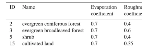
Table 1. Initial values of land-use-based parameters in Tiantoushui catchment.

ID Name Evaporation Roughness

coefficient coefficient

2 evergreen coniferous forest 0.7 0.4 3 evergreen broadleaved forest 0.7 0.6

5 shrub 0.7 0.4

15 cultivated land 0.7 0.35

catchment helps to keep the running time to a feasible limit. There are 50 rain gauges within the catchment and one river flow gauge in the catchment outlet. The high-density rain gauge network is built not only for flash flood forecasting but also for some kinds of scientific experiments. This will also help to reduce the uncertainties caused by the uneven precipitation spatial distribution. Figure 1a is the sketch map of Tiantoushui catchment with locations of rain gauges and the tributaries.

Hydrological data of nine flood events have been collected for this study, including the river flow at the catchment outlet and precipitation at each rain gauges at an hourly interval. The precipitation measured by the rain gauges will be in-terpolated to the grid cells by employing Thiessen polygon method (Derakhshan et al., 2011).

The second studied catchment is the upper portion of Wu-jiang catchment in southern China. It is called in this paper the upper and middle Wujiang catchment (UMWC). UMWC is in the upper and middle stream of Wujiang catchment with a drainage area of 3622 km2. Flooding in the catchment is also very frequent and heavy. The purpose of studying this big catchment is to show that PSO could still work in a large catchment. There is one river flow gauge in the out-let of UMWC and 17 rain gauges within the catchment. Fig-ure 1b shows the sketch map of the catchment with locations of rain gauges and the tributaries. Hydrological data of 14 flood events from UMWC have been collected, including the river flow at the catchment outlet and precipitation at each rain gauges at 1 h interval. The precipitation measured by the rain gauges will also be interpolated to the grid cells employ-ing Thiessen polygon method.

3.2 Property data for the Liuxihe model setup

(a)Tiantoushui Catchment

(b) Upper and middle Wujiang Catchment(UMWC) Figure 1sketch map of the studied Catchments

!

.

!

.

!

.

!

.

!

.

!

.

Baishi town Xinhua town

Chishi town

Qingyun town Huangpu town Yangmeishan town

±

01.753.5 7 10.5 14 Kilometers Legend

!

. Town Rain gauges

River

Boundary

!

.

!

.

!

.

!

.

!

.

!

.

!

.

!

.

!

.

!

.

!

.

!

.

!

.

!

.

!

.

!

.

!

.

!

.

!

.

Yiliu town Wushui town

Matian town

Liyuan town Pinghe town

Linwu county

Yinchun town

Meitian town

Pingshi town Chujiang town

Gangqiao town

Jinjiang town

Nanqiang town

Shuidong town Baishidu town

Huangsha town

Chengnan town

±

0 5 10 20 30 40

Kilometers Legend

!

. Town

Rain gauges

River

Boundary

Figure 1. Sketch map of the studied catchments: (a) Tiantoushui catchment and (b) upper and middle Wujiang catchment (UMWC).

the spatial resolution of 90 m×90 m. Figures 2 and 3 show the property data of DEM, land use types and soil types of the two catchments respectively.

Figure 2. Terrain properties of Tiantoushui catchment: (a) DEM, (b) land use type and (c) soil type.

In the Tiantoushui catchment, the highest, lowest and av-erage elevation are 1874, 174 and 782 m respectively. There are four land use types – evergreen coniferous forest, ever-green broadleaved forest, bush and farmland – accounting for 27.6, 36.5, 25.5, and 10.4 % of the total catchment area respectively. There are 10 soil types – water body, Humic Acrisol, Haplic and highly active Acrisol, Ferralic Cambisol, Haplic Luvisols, Dystric Cambisol, Calcaric Regosol, Dys-tric Regosol, Artificial accumulated soil and DysDys-tric rankers – accounting for 4.8, 56.5, 1.7, 3.4, 6.5, 4.5, 0.7, 5.6, 9.8 and 6.5 % of the total catchment area respectively.

Figure 3. Terrain property data of UMWC: (a) DEM, (b) land use type and (c) soil type.

4.8, 56.5, 0.5, 3.4, 6.5, 4.5, 0.7, 5.6, 9.8, 6.6, 1.0 and 0.2 % of the total catchment area respectively.

3.3 Liuxihe model setup

Setting up the Liuxihe model in the studied catchments con-sists of dividing the whole catchment into grids with DEM. In this study, the Tiantoushui catchment is divided into 65 011 grid cells using the DEM with grid cell size of 90 m×90 m; then they are categorized into reservoir cell, river channel cell and hillslope cell. In the studied catchments, there are no significant reservoirs, so there are no reservoir cells set. Based on the method for cell type classification proposed in the Liuxihe model, the river channel system is treated as a third-order channel system, and 1364 river channel cells and 63 647 hillslope cells have been produced in Tiantoushui catchment respectively. Further, 10 nodes have been set on the Tiantoushui catchment, and the river channel system is divided into 14 virtual sections. Their cross section sizes have been estimated by referencing to satellite remote-sensing im-ages. The Liuxihe model structure of Tiantoushui catchment is shown in Fig. 4a.

The Liuxihe model is also set up in UMWC. The catch-ment is first divided into 460 695 grid cells using the DEM with grid cell size of 90 m×90 m. The river channel sys-tem is treated as a third-order channel syssys-tem, and 3295 river channel cells and 457 400 hillslope cells have been produced respectively; 32 nodes have been set on UMWC, and their cross-section sizes have been estimated by referencing to

satellite remote sensing images. The Liuxihe model structure of UMWC is shown in Fig. 4b.

3.4 Determination of initial parameter values

In the Liuxihe model, the flow direction and slope are two un-adjustable parameters which will be derived from the DEM and will remain unchanged. Based on the DEM shown in Fig. 1a, the flow direction and slope of the studied catch-ments are derived. The other parameters are adjustable pa-rameters, which need initial values for further optimization. Evaporation capacity is a climate-based parameter, and its initial value is set to 5 mm d−1at both catchment based on the observation near the catchment outlet. Evaporation coef-ficient and roughness are land-use-based parameters and are less sensitive parameters in the Liuxihe model. The initial values of evaporation coefficient are set to 0.7 at both catch-ments as recommended by the Liuxihe model (Chen, 2009), while the initial values of roughness are derived based on Wang et al. (1997) and are listed in Tables 1 and 2 respec-tively for the two catchments.

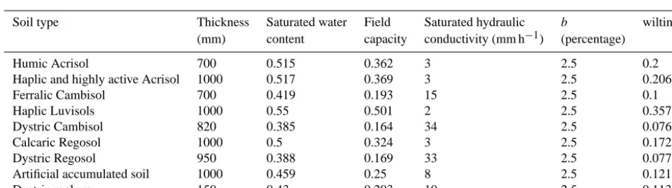
The other parameters are soil-based parameters. In the Li-uxihe model, b is recommended to take the value of 2.5. Soil water content under wilting conditions takes 30 % of the soil water content under saturated conditions. The initial val-ues of other soil-based parameters are calculated by using the Soil Water Characteristics Hydraulic Properties Calcula-tor (Arya et al., 1981), which calculates soil water content at saturation and field condition and the hydraulic conduc-tivity at saturation based on the soil texture, organic matter, gravel content, salinity and compaction. The initial values of soil-based parameters are determined by using the program developed by Keith E. Saxton that can be downloaded for free at http://hydrolab.arsusda.gov/soilwater/Index.htm. The initial values of the soil-based parameters at the two studied catchments are listed in Tables 3 and 4 respectively.

4 Discussion and results

4.1 Impacting of particle number to PSO performance and the determination of appropriate particle number

Ta-Table 2. Initial values of land-use-based parameters in UMWC.

ID Name Evaporation Roughness coefficient coefficient

2 Evergreen coniferous forest 0.7 0.4 3 Evergreen broadleaved forest 0.7 0.6

5 Shrub 0.7 0.4

6 Sparse wood 0.7 0.5

7 Mountains and alpine meadow 0.7 0.2 8 Slope grassland 0.7 0.3

10 Lakes 0.7 0.05

15 Cultivated land 0.7 0.35

Table 3. Initial values of soil-based parameters in Tiantoushui catchment.

Soil type Thickness Saturated water Field Saturated hydraulic b wilting (mm) content capacity conductivity (mm h−1) (percentage)

Humic Acrisol 700 0.515 0.362 3 2.5 0.2

Haplic and highly active Acrisol 1000 0.517 0.369 3 2.5 0.206

Ferralic Cambisol 700 0.419 0.193 15 2.5 0.1

Haplic Luvisols 1000 0.55 0.501 2 2.5 0.357

Dystric Cambisol 820 0.385 0.164 34 2.5 0.076

Calcaric Regosol 1000 0.5 0.324 3 2.5 0.172

Dystric Regosol 950 0.388 0.169 33 2.5 0.077

Artificial accumulated soil 1000 0.459 0.25 8 2.5 0.121

Dystric rankers 150 0.43 0.203 10 2.5 0.113

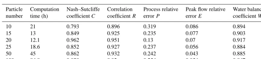
ble 5. The computation times for each optimization are also listed in Table 5.

We first analyze the impact of particle number on the com-putation time. From the results of Table 5 we found that with the increase of the particle number from 10 to 100, the computation time used decreases first. However, when the particle number is bigger than 20, the computation time in-creases then, and when the particle number is 20, the com-putation time is 12.1 h, which is the shortest among others. This means that particle number impacts the computation time used in optimization. The small and big particle number is not the best particle number. There exists an appropriate particle number to make the optimization in the least amount of time. In the Tiantoushui catchment, 20 is an appropriate particle number from the view of computational efficiency.

We further analyze the impact of particle number on the model performances by comparing the five evaluation in-dices. From the results, an obvious trend could be found: with the increase of the particle number, the Nash–Sutcliffe coef-ficient C, the correlation coefcoef-ficientRand water balance co-efficient increase first, but when the particle number reaches 20, the three indices decrease. However, for the process rel-ative error W and peak flow relative error E, the trend is inversed (i.e., with the increase of the particle number, the process relative errorW and peak flow relative errorE de-crease first, but when the particle number reaches 20, the two

indices increase). This also means that, with the increase of the particle number, the model performance increases first and then decreases. So from the view of model performance, we could assume 20 is the appropriate particle number in the Tiantoushui catchment. So in this paper, from the results above, we could suggest that 20 is the appropriate particle number of PSO algorithm for the Liuxihe model in catch-ment flood forecasting in Tiantoushui catchcatch-ment.

The particle number of 20 is also used in the parameter op-timization of UMWC catchment, and the model performance is also very satisfactory. The computation time is acceptable, so in this study we assume that 20 is the appropriate particle number for the Liuxihe model parameter optimization when employing the PSO algorithm for catchment flood forecast-ing no matter the size of the catchment. This conclusion can also be derived from the results of PSO’s convergence in the next section.

4.2 PSO’s convergence

Table 4. Initial values of soil-based parameters in UMWC.

Soil type Thickness Saturated water Field Saturated hydraulic b wilting (mm) content capacity conductivity (mm h−1) (percentage)

Humic Acrisol 700 0.515 0.362 3 2.5 0.2

Haplic and highly active Acrisol 1000 0.517 0.369 3 2.5 0.206

Ferralic Cambisol 700 0.419 0.193 15 2.5 0.1

Haplic Luvisols 1000 0.55 0.501 2 2.5 0.357

Dystric Cambisol 820 0.385 0.164 34 2.5 0.076

Calcaric Regosol 1000 0.5 0.324 3 2.5 0.172

Dystric Regosol 950 0.388 0.169 33 2.5 0.077

Haplic and weakly active Acrisol 1000 0.55 0.501 2 2.5 0.357 Artificial accumulated soil 1000 0.459 0.25 8 2.5 0.121 Eutric Regosols and black limestone soil 430 0.495 0.312 4 2.5 0.156

Dystric rankers 150 0.43 0.203 10 2.5 0.113

Table 5. Performances of PSO algorithm in Tiantoushui catchment.

Particle Computation Nash–Sutcliffe Correlation Process relative Peak flow relative Water balance number time (h) coefficientC coefficientR errorP errorE coefficientW

10 21 0.793 0.896 0.319 0.086 0.894

15 13 0.849 0.925 0.235 0.077 0.903

20 12.1 0.962 0.951 0.13 0.07 0.917

25 18.6 0.852 0.927 0.237 0.056 0.884

50 45 0.862 0.932 0.242 0.043 0.885

100 86.8 0.838 0.92 0.256 0.054 0.867

Tiantoushui catchment in Fig. 5. Both the objective and pa-rameter evolution processes are included.

From Fig. 5 we found that, during the evolution process, the objective function steadily decreases, which means the model performance is constantly improved. But for all the parameters, they do not change in the same direction: the parameters may increase in one evolution and decrease in the next evolution. However, after more than 25 evolutions, most of the parameters converge to their optimal values. With about 30 evolutions, all of the parameters converge to their optimal values; after that, there are almost no parameter changes. This means 30 is the maximum evolution number for PSO in Tiantoushui catchment.

From Fig. 5, we also found that the optimal parameter val-ues of several parameters are quite different with the initial parameters, but some remain little changes. This also implies that the PSO algorithm has very good performance in conver-gence. Even the initial values of the parameters are far from their optimal values.

We further analyze PSO’s performance in UMWC, but this time we only draw the parameter evolution process of PSO in UMWC in Fig. 6. The objective evolution process of PSO in UMWC is similar to that in the Tiantoushui catchment.

From Fig. 6 we also found that, during the evolution pro-cess, the objective function steadily decreases, but the pa-rameters do not increase or decrease in a constant way. The

changing patten is similar to that shown in Fig. 5. After 25 evolutions, most of the parameters converge to their optimal values. With about 30 evolutions, all of the parameters con-verge to their optimal values. The patten in UMWC is the same as that in Tiantoushui catchment.

From Fig. 6, we also found that the optimal parameter val-ues of several parameters are quite different from the initial values, but some remain little changes. This patten in UMWC is the same as that in Tiantoushui catchment also.

From the above results both in UMWC and Tiantoushui catchment, we could assume that PSO algorithm has a very good performance in convergence in catchments with differ-ent sizes, and we could assume that the maximum evolution number could be set to 30 no matter the size of the stud-ied catchments. This conclusion also supports the conclusion that 20 is the appropriate particle number for the Liuxihe model parameter optimization when employing PSO algo-rithm for catchment flood forecasting no matter the size of the catchment.

4.3 Computational efficiency

(a) Tiantoushui Catchment

(b) UMWC Catchment

2-2

3-6 2-1

1-2 3-5

3-4 3-3

3-2 3-1

1-1

±

0 2 4 8 12 16

Kilometers Legend

Virtual node

River

Boundary

!

.

!

.

!

.

!

.

!

.

!

.

!

.

!

.

!

.

!

.

!

.

!

.

!

.

!

.

!

.

!

.

!

.

!

.

!

.

!

.

!

.

!

.

!

.

!

.1-5

1-4

1-3

1-2 2-9 2-8 2-7

2-6 2-5 2-4 1-2

3-1 2-3

2-2 2-1 1-1

2-17

2-16 2-15

2-14 2-13

2-12 2-11 2-10

±

Kilometers Legend

!

. Virtual node

River

Boundary

Figure 4. Model setup results: (a) Tiantoushui catchment and (b) UMWC catchment.

Figure 5. The evolution process of parameter optimization with PSO in Tiantoushui catchment: (a) evolution of objective function and (b) evolution of parameters.

Figure 6. The evolution processes of parameter optimization with PSO in UMWC.

Figure 7. Simulated flood events of Tiantoushui Catchmen. (a) flood1996071012, (b) flood2001061206, (c) flood2008061114, (d) flood2012060901.

is a general server. If we used an advanced computer, the time needed could be reduced largely.

4.4 Model validation in Tiantoushui catchment

The parameters of the Liuxihe model in Tiantoushui catch-ment have been optimized by employing PSO algorithm proposed in this paper. The particle number used is 20. Maximum evolution number is set to 50; ω, C1 and C2 are dynamically adjusted with Eqs. (4)–(6). Flood event flood2006071409 is used to optimize the parameters.

The other eight observed flood events of Tiantoushui catchment are simulated by the model with parameters op-timized above to validate the model performance for catch-ment flood forecasting. To analyze the effect of parameter op-timization to model performance improvement, Fig. 7 shows four of the simulated hydrographs. The hydrographs sim-ulated by the model with initial parameter values are also drawn in Fig. 7.

From the results, it has been found that the eight simulated hydrographs fit the observed hydrographs well. Particularly the simulated peak flow is quite good. From the results we also found that the model with initial parameter values does

not simulate the observed flood events satisfactorily (i.e., the uncertainties are high).

To further analyze the model performance with parameter optimization, the five evaluation indices of the eight simu-lated flood events have been calcusimu-lated and are listed in Ta-ble 6.

From Table 6 we found that the five evaluation indices have been improved by parameter optimization at different extents. For the results simulated by the model with initial pa-rameters, the five evaluation indices – the Nash–Sutcliffe co-efficient, correlation coco-efficient, process relative error, peak flow relative error and water balance coefficient – have av-erage values of 0.66, 0.85, 72 %, 21 % and 1.03 respectively. For the results simulated by the model with optimized param-eters, the five evaluation indices have average values of 0.88, 0.94, 25 %, 6 % and 0.97 respectively. The average Nash– Sutcliffe coefficient has a 33 % increase, the correlation co-efficient a 9.6 % increase, process relative error a 65.28 % decrease, peak flow relative error a 71.43 % decrease, and the water balance coefficient a 5.83 % decrease. Among the five evaluation indices, the peak flow relative error and the process relative error have the biggest improvement.

Figure 8. Simulated flood events of UMWC: (a) flood1981040712, (b) flood1981041310, (c) flood1983022720 and (d) flood1987052012.

Table 6. The evaluation index of the simulated flood events in Tiantoushui catchment.

Nash–Sutcliffe Correlation Process relative Peak flow relative Water balance coefficientC coefficientR errorP(%) errorE(%) coefficientW

Flood events (1)∗1 (2)∗2 (1)∗1 (2)∗2 (1)∗1 (2)∗2 (1)∗1 (2)∗2 (1)∗1 (2)∗2

flood1996071012 0.964 0.85 0.990 0.79 16.3 30 11.2 15.6 1.102 2.19 flood1998061811 0.862 0.613 0.930 0.876 21.4 194.6 20.8 39.7 0.963 1.194 flood2001061206 0.836 0.758 0.926 0.969 31.8 35 0.9 31.1 0.841 0.64 flood2007082100 0.866 0.343 0.942 0.775 13.9 40.9 0.7 32.9 0.966 0.581 flood2008061114 0.882 0.74 0.943 0.883 20.8 71 2.5 31 0.930 0.36 flood2012040607 0.792 0.766 0.893 0.891 27.0 76.4 5.0 11.5 0.913 1.058 flood2012060901 0.912 0.454 0.958 0.752 37.0 74.5 3.2 1.5 1.072 1.238 flood2012062113 0.91 0.778 0.955 0.896 0.301 49.8 0.005 8.4 0.972 0.987

Average 0.88 0.66 0.94 0.85 25 72 6 21 0.97 1.03

∗_{1: results simulated by model with optimized parameters,}∗_{2: results simulated by model with initial parameters.}

performance of the Liuxihe model for catchment flood fore-casting has been improved in Tiantoushui catchment. Opti-mizing the parameters of the Liuxihe model is necessary.

4.5 Model validation in UMWC

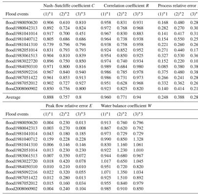
Table 7. The evaluation index of the simulated flood events in UMWC.

Nash–Sutcliffe coefficientC Correlation coefficientR Process relative errorP

Flood events (1)∗1 (2)∗2 (3)∗3 (1)∗1 (2)∗2 (3)∗3 (1)∗1 (2)∗2 (3)∗3

flood1980050620 0.906 0.610 0.810 0.958 0.831 0.931 0.168 0.480 0.288 flood1980042313 0.892 0.724 0.824 0.972 0.768 0.968 0.282 0.270 0.307 flood1981041014 0.917 0.700 0.451 0.967 0.830 0.883 0.141 0.417 0.317 flood1981040712 0.805 0.686 0.686 0.964 0.738 0.938 0.154 0.550 0.255 flood1981041310 0.739 0.796 0.796 0.938 0.758 0.958 0.221 0.260 0.265 flood1982051014 0.831 0.793 0.793 0.924 0.852 0.952 0.271 0.440 0.174 flood1983061513 0.904 0.810 0.839 0.954 0.850 0.925 0.327 0.530 0.363 flood1983022720 0.896 0.750 0.850 0.974 0.740 0.934 0.152 0.220 0.102 flood1984050310 0.971 0.800 0.816 0.989 0.684 0.980 0.085 0.380 0.388 flood1985092216 0.967 0.840 0.940 0.986 0.785 0.978 0.375 0.480 0.380 flood1987051422 0.961 0.853 0.913 0.986 0.731 0.973 0.266 0.241 0.281 flood1987052012 0.902 0.727 0.927 0.951 0.628 0.968 0.332 0.362 0.262 flood2008060902 0.850 0.756 0.800 0.923 0.825 0.820 0.140 0.414 0.214

Average 0.888 0.757 0.8 0.960 0.771 0.94 0.248 0.388 0.28

Peak flow relative errorE Water balance coefficientW

Flood events (1)∗1 (2)∗2 (3)∗3 (1)∗1 (2)∗2 (3)∗3

flood1980050620 0.004 0.230 0.013 0.913 0.760 0.796 flood1980042313 0.003 0.270 0.008 0.867 0.620 0.792 flood1981041014 0.043 0.180 0.185 0.973 0.729 0.729 flood1981040712 0.159 0.228 0.228 0.990 0.850 1.328 flood1981041310 0.006 0.146 0.146 0.830 1.160 1.061 flood1982051014 0.013 0.230 0.230 0.922 1.230 1.010 flood1983061513 0.007 0.350 0.072 0.944 0.680 0.967 flood1983022720 0.018 0.420 0.078 1.017 0.650 1.045 flood1984050310 0.010 0.210 0.010 0.951 0.720 0.820 flood1985092216 0.022 0.320 0.055 1.071 1.350 1.034 flood1987051422 0.012 0.280 0.013 0.925 1.510 0.892 flood1987052012 0.015 0.160 0.034 0.955 0.840 0.979 flood2008060902 0.004 0.240 0.104 0.985 0.910 0.850

Average 0.024 0.251 0.09 0.949 0.924 0.95

∗_{1: results simulated by model with optimized parameters,}∗_{2: results simulated by model with initial parameters,}∗_{3: results simulated by}

model with half-automated optimized parameters.

are dynamically adjusted with Eqs. (4)–(6). Flood event flood1985052618 is used to optimize the parameters.

The other 13 observed flood events of UMWC are sim-ulated by the model with parameters optimized above. Fig-ure 8 shows four of the simulated hydrographs. To compare, the flood events also have been simulated with the parameters optimized with a half-automated parameter adjusting method (Chen, 2009), and the results are also shown in Fig. 8. From the simulated results, it has been found that the 13 simulated hydrographs fit the observed hydrographs well. Particularly the simulated peak flow is quite good. This conclusion is the same as the results in the Tiantoushui catchment. From the results we also found that the model with initial parameter values does not simulate the observed flood event satisfac-torily. The simulated results with parameters optimized with a half-automated parameter adjusting method are a big

im-provement to those simulated with the initial model parame-ters, but the simulated results with the PSO optimized model parameters are the best among the three results.

To further analyze the model performance with parameter optimization, the five evaluation indices of the 13 simulated flood events have been calculated and are listed in Table 7.

respec-tively. The peak flow relative error has been reduced from 25.1 to 2.4 % after parameter optimization, which is 90.44 % down and also the biggest improvement among the five eval-uation indices. The average Nash–Sutcliffe coefficient has a 17.31 % increase, the correlation coefficient a 24.51 % in-crease, process relative error a 36.08 % decrease and water balance coefficient a 2.71 % increase. The results have a silar trend to that in the Tiantoushui catchment. This also im-plies that with parameter optimization by using the PSO al-gorithm proposed in this paper, the model performance of the Liuxihe model for catchment flood forecasting has been improved in UMWC catchment: even for a larger catchment, PSO works well for the Liuxihe model. The Liuxihe model’s capability for catchment flood forecasting could be improved by parameter optimization with PSO algorithm, and the Li-uxihe model parameter optimization is necessary.

5 Conclusion

In this study, based on the scalar concept, a general frame-work for automatic parameter optimization of the physically based distributed hydrological model is proposed, and the improved particle swarm optimization algorithm is employed for the Liuxihe model parameter optimization for catchment flood forecasting. The proposed methods have been tested in two catchments in southern China with different sizes: one small and one large. Based on the study results, the follow-ing conclusions can be drawn:

1. When employing physically based distributed hydro-logical model for catchment flood forecasting, uncer-tainty in deriving model parameters physically from the terrain properties is high. Parameter optimization is still necessary to improve the model’s capability for catch-ment flood forecasting.

2. Capability of physically based distributed hydrological model for catchment flood forecasting, specifically the Liuxihe model studied in this paper, could be improved largely by parameter optimization with PSO algorithm, and the model performance is quite good with the opti-mized parameters to satisfy the requirement of real-time catchment flood forecasting.

3. Improved particle swarm optimization (PSO) algorithm proposed in this paper for physically based distributed hydrological model for catchment flood forecasting, specifically the Liuxihe model studied in this paper, has very good optimization performance. The optimized model parameters are global optimal parameters and could be used for the Liuxihe model parameter opti-mization for catchment flood forecasting at different size catchments.

4. The appropriate particle number of PSO algorithm used for the Liuxihe model parameter optimization for catch-ment flood forecasting is 20.

5. The maximum evolution number of PSO algorithm used for the Liuxihe model parameter optimization for catch-ment flood forecasting is 30.

6. The PSO algorithm has high computational efficiency and could be used in large-scale catchment flood fore-casting.

Acknowledgements. This study is supported by the Special Research Grant for the Water Resources Industry (funding no. 201301070), the National Science & Technology Pillar Program during the Twentieth Five-year Plan Period (funding no. 2012BAK10B06), the Science and Technology Program of Guangdong Province (funding no. 2013B020200007) and Water Resources Science Program of Guangdong Province (funding no. 2009-16).

Edited by: Y. Chen

References

Abbott, M. B., Bathurst, J. C., Cunge, J. A., O’Connell, P. E., and Rasmussen, J.: An Introduction to the European Hydrologic System-System Hydrologue Europeen, ‘SHE’, a: History and Philosophy of a Physically-based, Distributed Modelling Sys-tem, J. Hydrol., 87, 45–59, 1986a.

Abbott, M. B.,Bathurst, J. C.,Cunge, J. A.,O’Connell, P. E., and Rasmussen, J.: An Introduction to the European Hydrologic System-System Hydrologue Europeen, ‘SHE’, b: Structure of a Physically based, distributed modeling System, J. Hydrol., 87, 61–77, 1986b.

Acharjee, P. and Goswami, S. K.: Chaotic particle swarm optimiza-tion based robust load flow, Int. J. Electr. Power Energ. Syst., 32, 141–146, 2010.

Ajami, N. K., Gupta, H., Wagener, T., and Sorooshian, S.: Calibra-tion of a semi-distributed hydrologic model for streamflow esti-mation along a river system, J. Hydrol., 298, 112–135, 2004. Ambroise, B., Beven, K., and Freer, J.: Toward a generalization of

the TOPMODEL concepts: Topographic indices of hydrologic similarity, Water Resour. Res., 32, 2135–2145, 1996.

Arnold, J. G., Williams, J. R., and Srinivasan, R.: SWAT: Soil water assessment tool, US Department of Agriculture, Agricultural Re-search Service, Grassland, Soil and Water ReRe-search Laboratory, Temple, Texas, USA, 1994.

Arya, L. M. and Paris, J. F.: An empirical model to predict the soil moisture characteristic from particle-size distribution and bulk density data, Soil Sci. Soc. Am. J., 45, 1023–1030, 1981. Bahareh, K. S., Mousavi, J., and Abbaspour, K. C.: Automatic

cali-bration of HEC-HMS using single-objective and multi-objective PSO algorithms, Hydrol. Process., 27, 4028–4042, 2013. Beven, K., Lamb, R., Quinn, P., Romanowicz, R., and Freer, J.:

Carpenter, T. M., Georgakakos, K. P., and Sperfslagea, J. A.: On the parametric and NEXRAD-radar sensitivities of a distributed hydrologic model suitable for operational use, J. Hydrol., 253, 169–193, 2001.

Chen, G., Jia, J., and Han, Q.: Study on the Strategy of Decreasing Inertia Weight in Particle Swarm Optimization Algorithm, Jour-nal of Xi’an Jiantong University, 40, 53–56, 2006.

Chen, S., Cai, G. R., Guo, W. Z., and Chen, G. L.: Study on the Nonlinear Strategy of Acceleration Coefficient in Particle Swarm Optimization (PSO) Algorithm, Journal of Yangtze University (Nat. Sci. Edit), 1–4, 2007.

Chen, Y.: Liuxihe Model, Beijing, Science Press, 198 pp., 2009. Chen, Y., Zhu, X., Han, J., and Cluckie, I.: CINRAD data quality

control and precipitation estimation, Water Manage., 162, 95– 105, 2009.

Chen, Y., Ren, Q. W., Huang, F. H., Xu, H. J., and Cluckie, I.: Liux-ihe Model and its modeling to river basin flood, J. Hydrol. Eng., 16, 33–50, 2011.

Chu, W., Gao, X., and Sorooshian, S.: A new evolutionary search strategy for global optimization of high-dimensional problems, Inf. Sci., 181, 4909–4927, 2011.

Chuang, L. Y., Hsiao, C. J., and Yang, C. H.: Chaotic particle swarm optimization for data clustering, Expert Syst. Appl., 38, 14555– 14563, 2011.

Crawford, N. H. and Linsley, R. K.: Digital simulation in hydrology, Stanford Watershed Model IV, Stanford Univ. Dep. Civ. Eng, Tech. Rep., 39, 1966.

De Smedt, F., Liu, Y. B., and Gebremeskel, S.: Hydrological mod-eling on a watershed scale using GIS and remote sensed land use information, edited by: Brebbia, C. A., in: Risk Analyses, WIT press, Southampton, Boston, p. 10, 2000.

Derakhshan, H. and Talebbeydokhti, N.: Rainfall disaggregation in non-recording gauge stations using space-time information sys-tem, Sci. Iran., 18, 995–1001, 2011.

Dorigo, M., Maniezzo, V., and Colorni, A.: Ant system: optimiza-tion by a colony of cooperating agents. Systems, Man, and Cy-bernetics, Part B: CyCy-bernetics, IEEE Trans., 26, 29–41, 1996. Duan, Q., Sorooshian, S., and Gupta, V. K.: Optimal use of the

SCE-UA global optimization method for calibrating watershed mod-els, J. Hydrol., 158, 265–284, 1994.

Eberhart, R. C. and Shi, Y.: Tracking and optimizing dy-namic systems with particle swarms, IEEE, 1, 94–100, doi:10.1109/CEC.2001.934376, 2001.

Eberhart, R. C. and Shi, Y.: Particle swarm optimization: developments, applications and resources, IEEE, 1, 81–86, doi:10.1109/CEC.2001.934374, 2001.

El-Gohary, A., Al-Ruzaiza, A. S.:Chaos and adaptive control in two prey, one predator system with nonlinear feedback, Chaos, Soli-tons & Fractals, 34, 443–453, 2007.

Falorni, G., Teles, V., Vivoni, E. R., Bras, R. L., and Amaratunga, K. S.: Analysis and characterization of the vertical accuracy of digital elevation models from the Shuttle Radar Topogra-phy Mission, J. GeoTopogra-phys. Res. F-Earth Surf., 110, F02005, doi:10.1029/2003JF000113, 2005.

Franchini, M.: Use of a genetic algorithm combined with a local search for the automatic calibration of conceptual rainfall-runoff models, Hydrological Sciences Journal, 41, 21–39, 1996.

Freeze, R. A. and Harlan, R. L.: Blueprint for a physically-based, digitally simulated, hydrologic response model, J. Hydrol., 9, 237–258, 1969.

Fulton R. A., Breidenbach J. P. and Seo D-J., Miller, D. A.: The WSR-88D rainfall algorithm, Weather Forecast., 13, 377–395, 1998.

Goldberg, D. E.: Genetic algorithms in search, optimization and ma-chine learning, Reading, MA, Addison-Wesley, 95–99, 1989. Grayson, R. B., Moore, I. D., and McMahon, T. A.: Physically based

hydrologic modeling: 1.A Terrain-based model for investigative purposes, Water Resour. Res., 28, 2639-2658, 1992.

Gupta, H. V., Sorooshian, S., and Yapo, P. O.: Toward im-proved calibration of hydrological models: multiple and non-commensurable measures of information, Water Resour. Res., 34, 751–763, 1998.

Hendrickson, J. D., Sorooshian, S., and Brazil, L. E.: Comparison of Newton-type and direct search algorithms for calibration of conceptual rainfall-runoff models, Water Resour. Res., 24, 691– 700, 1988.

Holland, J. H.: Adaptation in natural and artificial systems:An intro-ductory analysis with applications to biology, control, and artifi-cial intelligence, Cambridge, MA, University of Michigan Press, ISBN:0262082136, 1992.

Hooke, R. and Jeeves, T. A.: “Direct Search” Solution of Numerical and Statistical Problems, JACM, 8, 212–229, 1961.

Ibbitt, R. P. and O’Donnell, T.: Designing conceptual catchment models for automatic fitting methods, IAHS Publication, 101, 462–475, 1971.

Immerzeel, W. W. and Droogers, P.: Calibration of a distributed hydrological model based on satellite evapotranspiration, J. Hy-drol., 349, 411–424, 2008.

Jasper , A.. Vrugt, H. V., and Gupta, W. B.:A Shuffled Complex Evolution Metropolis algorithm for optimization and uncertainty assessment of hydrologic model parameters, Water Resour. Res., 39, 1201, doi:10.1029/2002WR001642, 2003.

Jeraldin, A. D. and Anitta, T.: PSO tuned PID-based Model Ref-erence Adaptive Controller for coupled tank system, Applied Mechanics and Materials Trans Tech Publications, Switzerland, doi:10.4028/www.scientific.net/AMM.626.167, 626 pp., 167– 171, 2014.

Jia, Y., Ni, G., and Kawahara, Y.: Development of WEP model and its application to an urban watershed, Hydrol. Process., 15, 2175–2194, 2001.

Julien, P. Y., Saghafian, B., and Ogden, F. L.: Raster-Based Hydro-logic Modeling of spatially-Varied Surface Runoff, Water Re-sour. Bulletin, 31, 523–536, 1995.

Kavvas, M., Chen, Z., Dogrul, C., Yoon, J., Ohara, N., Liang, L., Aksoy, H., Anderson, M., Yoshitani, J., Fukami, K., and Matsuura, T.: Watershed Environmental Hydrology (WEHY) Model Based on Upscaled Conservation Equations: Hydrologic Module, J. Hydrol. Eng., 9, 450–464, doi:10.1061/(ASCE)1084-0699, 2004.

Kennedy, J. and Eberhart, R.: Particle swarm optimization: Proceed-ings, IEEE International Conference on Neural Networks, Picat-away NJ, IEEE Service Center, 1942–1948, 1995.

Kirkpatrick, S., Gelatt, C. D., and Vecchi, M.: Optimization by sim-ulated annealing, Science, 220, 671–680, 1983.

Kouwen, N.: WATFLOOD: A Micro-Computer based Flood Fore-casting System based on Real-Time Weather Radar, Canad. Wa-ter Resour. J., 13, 62–77, 1988.

Laloy, E., Fasbender, D., and Bielders, C. L.: Parameter optimiza-tion and uncertainty analysis for plot-scale continuous modeling of runoff using a formal Bayesian approach, J. Hydrol., 380, 82– 93, 2010.

Leila, O. , Miguel, A., and Mariño, A. A.: Multi-reservoir Operation Rules: Multi-swarm PSO-based Optimization Approach, Water Resour. Manage., 26, 407–427, 2012.

Leta O. T, Nossent J., Velez C., Shrestha N. K., Griensven, A., and Bauwens W.: Assessment of the different sources of uncertainty in a SWAT model of the River Senne (Belgium), Environ. Model. Softw., 68, 129–146, 2015.

Li, X., Chun, C., Xin, W., and Jian, L.: Study on Fuzzy Multi-objective SCE-UA Optimization Method for Rainfall-Runoff Models, Eng. Sci., 3, 52–57, 2007.

Liang, X., Lettenmaier, D. P., Wood, E. F., and Burges, S. J.: A simple hydrologically based model of land surface water and en-ergy fluxes for general circulation models, J. Geophys. Res, 99, 14415–14428, 1994.

Loveland, T. R., Merchant, J. W., Ohlen, D. O., and Brown, J. F.: Development of a Land Cover Characteristics Data Base for the Conterminous U.S., Photogram. Eng. Remote Sens., 57, 1453– 1463, 1991.

Loveland, T. R., Reed, B. C., Brown, J. F., Ohlen, D. O., Zhu, J., Yang, L., and Merchant, J. W.: Development of a Global Land Cover Characteristics Database and IGBP DISCover from 1-km AVHRR Data, Int. J. Remote Sens., 21, 1303–1330, 2000. Madsen, H.: Parameter estimation in distributed hydrological

catch-ment modelling using automatic calibration with multiple objec-tives, Adv. Water Resour., 26, 205–216, 2003.

Masri, S. F., Bekey, G. A., and Safford, F. B.: A global optimization algorithm using adaptive random search, Appl. Math. Comput., 7, 353–375, 1980.

Nash, J. E. and Sutcliffe, J. V.: River flow forecasting through con-ceptual models part – A discussion of principles, J. Hydrol., 10, 282–290, 1970.

Nelder, J. A. and Mead, R.: A simple method for function mini-mization, Comp. Journey, 7, 308–313, 1965.

O’Connell, P. E, Nash, J. E., and Farrell, J. P.: River flow forecast-ing through conceptual models part – The Brosna catchment at Ferbane, J. Hydrol., 10, 317–329, 1970.

Pokhrel, P., Gupta, H. V., and Wagener, T.: A spatial reg-ularization approach to parameter estimation for a dis-tributed watershed model, Water Resour. Res., 44, W12419, doi:10.1029/2007WR006615, 2008.

Pokhrel, P., Yilmaz, K. K., Gupta, H. V.: Multiple-criteria calibra-tion of a distributed watershed model using spatial regularizacalibra-tion and response signatures, J. Hydrol., 418–419, 49–60, 2012. Poli, R.: Analysis of the publications on the applications of particle

swarm optimisation. Journal of Artificial Evolution and Applica-tions, 1-10, 2008.

Poli, R., Kennedy, J., and Blackwell, T.: Particle swarm optimiza-tion. Swarm Intelligence, 1, 33–57, 2007.

Ratnaweera, A., Halgamuge, S. K., and Watson, H. C.: Self-organizing hierarchical particle swarm optimizer with time-varying acceleration coefficients, Evolutionary Computation, IEEE Trans., 8, 240–255, 2004.

Reed, S., Koren, V., Smith, M., Zhang, Z., Moreda, F., and Seo, D.-J.: DMIP participants: Overall distributed model intercomparison project results, J. Hydrol., 298, 27–60, 2004.

Refsgaard, J. C. and Storm, B.: Construction, calibration and valida-tion of hydrological models, in: Distributed Hydrological Mod-elling, edited by: Abbott, M. B. and Refsgaard, J. C., Kluwer Academic, Springer Netherlands, 41–54, 1996.

Refsgaard, J. C.: Parameterisation, calibration and validation of dis-tributed hydrological models, J. Hydrol., 198, 69–97, 1997. Resffa, F., O’ Castillo., Fevrier, V., and Leticia, C.: Design of

Op-timal Membership Functions for Fuzzy Controllers of the Wa-ter Tank and Inverted Pendulum with PSO Variants, IFSA World Congress and NAFIPS Annual Meeting (IFSA/NAFIPS), 1068– 1073, 2013.

Rosenbrock, H. H.: An automatic method for finding the greatest or least value of a function, Comp. Journey, 3, 175–184, 1960. Richard, A., Annie, P., Pascal, C., and François, B.:

Com-parison of Stochastic Optimization Algorithms in Hydrologi-cal Model Calibration, American Society of Civil Engineers, doi:10.1061/(ASCE)HE.1943-5584.0000938, 1374–1384, 2014. Shafii, M. and De Smedt, F.: Multi-objective calibration of a dis-tributed hydrological model (WetSpa) using a genetic algorithm, Hydrol. Earth Syst. Sci., 13, 2137–2149, doi:10.5194/hess-13-2137-2009, 2009.

Sharma, A. Tiwari, K. N.: A comparative appraisal of hydrologi-cal behavior of SRTM DEM at catchment level, J. Hydrol., 519, 1394–1404, 2014.

Sherman, L. K.: Streamflow from Rainfall by the Unit-Graph Method, Eng. News-Rec., 108, 501–505 1932.

Shi, Y. and Eberhart, R. C.: A modified particle swarm optimizer, IEEE, 69–73, doi:10.1109/ICEC.1998.699146, 1998.

Shi, Y. and Eberhart, R. C.: Fuzzy adaptive particle swarm optimiza-tion, IEEE, 1, 101–106, doi:10.1109/CEC.2001.934377, 2001. Shu, X. J., Chen, Y. B., Huang, F. H., and Zhou, H. L.:

Applica-tion of PEST in the Parameter CalibraApplica-tion of Wetspa Distributed Hydrological Model, J. China Hydrol., 29, 45–49, 2009. Singh, V. P.: Computer Models of Watershed Hydrology, Water

Resources Publications, Colorado, 1130, ISBN:0-918334-91-8, 1995.

Smith, M. B., Seo, D.-J., Koren, V. I., Reed, S., Zhang, Z., Duan, Q.-Y., Cong, S., Moreda, F., and Anderson, R.: The distributed model intercomparison project (DMIP): motivation and experi-ment design, J. Hydrol., 298, 4–26, 2004.

Song, S. L., Kong, L., Gan, Y., and Rijian, S. B.: Hybrid particle swarm cooperative optimization algorithm and its application to MBC in alumina production, Prog. Natural Sci., 18, 1423–1428, 2008.

Sorooshian, S., Gupta, V. K.:Model calibration. In: Singh VP, edi-tor. Computer models of watershed hydrology, Colorado, Water Resources Publications, 23–68, 1995.

Storn, R. and Price, K.: Differential evolution e a simple and effi-cient heuristic for global optimization over continuous spaces, J. Global Opt., 11, 341–359, 1997.

Tang, Y., Reed, P., and Wagener, T.: How effective and effi-cient are multiobjective evolutionary algorithms at hydrologic model calibration?, Hydrol. Earth Syst. Sci., 10, 289–307, doi:10.5194/hess-10-289-2006, 2006.

Vieux, B. E.: Distributed Hydrologic Modeling Using GIS, sec-ond ed. Water Science Technology Series, vol. 48. ISBN:1-4020-2459-2, Kluwer Academic Publishers, Norwell, Massachusetts, p. 289, 2004.

Vieux, B. E. and Moreda, F. G.: Ordered physics-based parame-ter adjustment of a distributed model, in: Advances in Calibra-tion of Watershed Models, edited by: Duan, Q., Sorooshian, S., Gupta, H. V., Rousseau, A. N., Turcotte, R., Water Science and Application Series, vol. 6. American Geophysical Union, 267– 281, ISBN:0-87590-335-X (Chapter 20), 2003.

Vieux, B. E. and Vieux, J. E.: Vflo™: A Real-time Distributed Hy-drologic Model[A], in: Proceedings of the 2nd Federal Intera-gency Hydrologic Modeling Conference, 28 July–1 August, Las Vegas, Nevada, Abstract and paper on CD-ROM, 2002.

Vieux, B. E., Cui, Z., and Gaur, A.: Evaluation of a physics-based distributed hydrologic model for flood forecasting, J. Hydrol., 298, 155–177, 2004.

Wigmosta, M. S., Vai, L. W., and Lettenmaier, D. P.: A Distributed Hydrology-Vegetation Model for Complex Terrain, Water Re-sour. Res., 30, 1665–1669, 1994.

Vrugt, J. and Robinson, B.: Improved evolutionary optimization from genetically adaptive multimethod search, P. Natl. Acad. Sci. USA, 104, 708–711, 2007.

Wang, Z., Batelaan, O., and De Smedt, F.: A distributed model for water and energy transfer between soil, plants and atmosphere (WetSpa), J. Phys. Chem. Earth, 21, 189–193, 1997.

Yang, D., Herath, S., and Musiake, K.: Development of a geomor-phologic properties extracted from DEMs for hydrologic model-ing, Ann. J. Hydr. Eng., JSCE, 47, 49–65, 1997.

Zambrano-Bigiarini, M. and Rojas, R.: A model-independent Parti-cle Swarm Optimisation software for model calibration, Environ. Model. Softw., 43, 5–25, 2013.

Zhang, X., Srinivasan, R., and Liew, M. V.: Multi-site calibration of the SWAT model for hydrologic modeling, Transactions of the ASABE, 51, 2039–2049, 2008.