A mechanistic description of the formation and evolution of vegetation patterns

www.hydrol-earth-syst-sci.net/17/63/2013/ doi:10.5194/hess-17-63-2013

© Author(s) 2013. CC Attribution 3.0 License.

Earth System

Sciences

A mechanistic description of the formation

and evolution of vegetation patterns

R. Foti1,*and J. A. Ram´ırez1

1_{Department of Civil and Environmental Engineering, Colorado State University, Fort Collins, Colorado, USA} *_{now at: Department of Civil and Environmental Engineering, Princeton University, Princeton, New Jersey, USA}

Correspondence to: R. Foti ([email protected])

Received: 6 June 2012 – Published in Hydrol. Earth Syst. Sci. Discuss.: 19 July 2012 Revised: 2 December 2012 – Accepted: 11 December 2012 – Published: 11 January 2013

Abstract. Vegetation patterns are a common and well-defined characteristic of many landscapes. In this paper we explore some of the physical mechanisms responsible for the establishment of self-organized, non-random vegetation patterns that arise at the hillslope scale in many areas of the world, especially in arid and semi-arid regions. In do-ing so, we provide a fundamental mechanistic understand-ing of the dynamics of vegetation pattern formation and de-velopment. Reciprocal effects of vegetation on the hillslope thermodynamics, runoff production and run-on infiltration, root density, surface albedo and soil moisture content are analyzed. In particular, we: (1) present a physically based mechanistic description of processes leading to vegetation pattern formation; (2) quantify the relative impact of each process on pattern formation; and (3) describe the relation-ships between vegetation patterns and the climatic, hydraulic and topographic characteristics of the system. We validate the model by comparing simulations with observed natural patterns in the areas of Niger near Niamey and Somalia near Garoowe. Our analyses suggest that the phenomenon of pat-tern formation is primarily driven by run-on infiltration and mechanisms of facilitation/inhibition among adjacent vegeta-tion groups, mediated by vegetavegeta-tion effects on soil properties and controls on soil moisture and albedo. Nonetheless, even in presence of those mechanisms, patterns arise only when the climatic conditions, particularly annual precipitation and net radiation, are favorable.

1 Introduction

The presence of self-organized vegetation patterns is a com-mon and well-defined characteristic of many arid and semi-arid landscapes. Indeed, vegetation is in general spatially het-erogeneous and its constituent species show spatial distribu-tions that depart from complete randomness (Greig-Smith, 1979), although only in a few cases, where this departure is more marked, the pattern structure is easily recognizable.

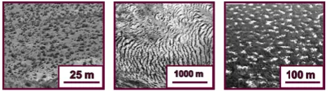
Vegetation patterns exhibit a multitude of shapes (banded, spotted or labyrinthine) and occur at a wide variety of spatial scales. Typical dimensions of a vegetation pattern element (i.e., width of a band or radius of a patch of vegetation) can span up to two orders of magnitude, ranging from 100m to almost 102m (Rietkerk and Van de Koppel, 2008).

Plants, especially in arid landscapes, help reduce soil ero-sion and augment soil permeability; they also protect each other from winds and damage caused by animals and ex-treme temperatures and humidity conditions. In some areas, these interactions favor the formation of bands of vegetation perpendicular to the planar slope vector in mild hillslopes (Bromley et al., 1997) or perpendicular to the direction of the prevalent winds in response to their erosive action (Lep-run, 1999). Although hillslope-scale patterns can arise in a variety of regions and climates, scarcity of water seems to be the common denominator of every landscape characterized by observable vegetation patterns.

Many models have been developed to describe vegetation structures that deviate from randomness. Cellular automata models, for example, have been successfully adopted to in-vestigate the spatial distribution of Acacia trees in desertic areas, (Wiegand et al., 1999, 2000) or to analyze gap dynam-ics and cohesistence of trees and grass in savannas (Jeltsch et al., 1996). However, most of the models that have been used specifically to reproduce the geometric vegetation struc-tures that are the objects of this study belong to three cate-gories: (1) kernel based models (Lefever and Lejeune, 1997; Thi´ery et al., 1995; D’Odorico et al., 2006); (2) advection– diffusion models (HilleRisLambers et al., 2001; Rietkerk et al., 2002); and (3) differential flow instability models (Klaus-meier, 1999; Sherrat, 2005; Saco et al., 2007). With this ef-fort, we intend to investigate vegetation pattern formation using a mechanistic water balance model coupled to phe-nomenological conceptualizations of the feedbacks among the components of the climate–soil–vegetation system. Our overarching objective is to explore and identify (some of) the physical mechanisms responsible for the establishment of non-random spatial vegetation patterns that arise in arid and semi-arid regions. In order to do so, we (1) develop a physically based mechanistic understanding of the pro-cesses leading to vegetation pattern formation; (2) implement such understanding in a mathematical model able to repli-cate the main physical characteristics of observed vegetation patterns; (3) individuate the relative importance of each pro-cess in pattern formation; and (4) capture the relationships between vegetation patterns and the climatic, hydraulic and topographic characteristics of the system.

2 Hypotheses

By “vegetation patterns” we refer to the non-random arrange-ment of vegetated and bare patches of soil on the landscape, where non-randomness indicates any spatial distribution of patches that deviates from a purely spatially random distri-bution.

Our first hypothesis is that vegetation patterns emerge as a result of physical, chemical and physiological feedbacks be-tween vegetation, hydrologic and climatic processes, and soil

Fig. 1. Vegetation patterns typical shapes and dimensions (edited

from D’Odorico et al., 2006).

properties, and that those feedback processes are amenable to quantitative description and modeling.

Our second hypothesis is that patterns develop because those feedback processes tend to make certain regions in the neighborhood of an existing clump of vegetation more con-ducive to the establishment of additional vegetation (or not). Finally, our third hypothesis is that the spatial distribu-tion of vegetadistribu-tion depends on the spatial distribudistribu-tion of soil moisture and energy (which, in turn, is influenced by the vegetation itself). Thus, physiological and hydrologi-cal processes conducive to lohydrologi-cal decreases in the available soil water and nutrients will tend to inhibit vegetation es-tablishment and those conducive to locally maintaining or increasing soil water and nutrients will tend to promote vegetation establishment.

In general, the previous hypotheses imply that the spatial structuring of vegetation is the result of a series of process that optimize the use of the available resources (Schymanski et al., 2009, 2010)

3 Methods

We are interested in analyzing vegetation agglomerates emerging at the hillslope scale and whose typical dimen-sions are of the order of magnitude of 100 to almost 102m (Fig. 1). Hence, we simulate the climate–soil–vegetation dy-namics of a hillslope on a two-dimensional gridded domain of area 105–107m2. In order to characterize self-organized spatial structures, we subdivide the study domain into a grid of pixels of area 100–102m2.

Although observed vegetation patterns show variability over time, their statistical properties do not change drasti-cally within a year and from year to year, suggesting that patterns are the result of adaptation to the long-term av-erage characteristics of the soil–climate system rather than a response to short-term disturbances. Under the assump-tion of staassump-tionary climate, therefore, we use long-term aver-age climatic and hydraulic conditions in order to determine the spatial configurations of vegetation and associated water and energy fluxes that are in long-term equilibrium with the soil–climate system.

3.1 Procedure schematization

Because the long-term average vegetation density (i.e., the portion of a given area which is covered by vegetation) at a certain location in space is the long-term response of the climate–soil–vegetation system to a set of environmen-tal forcings (e.g., precipitation, temperature, solar radiation), knowledge of the spatial arrangement of the environmental forcings over a certain domain can be used to determine the configuration of vegetation density over the same domain. Therefore, we seek to determine a spatial configuration of fluxes and vegetation density that simultaneously satisfies the water and energy budgets both at the global (i.e., for the en-tire study domain) and the local (i.e., for each pixel) scales, while taking into account lateral interactions (i.e., between adjacent pixels) between vegetation, climate and soil.

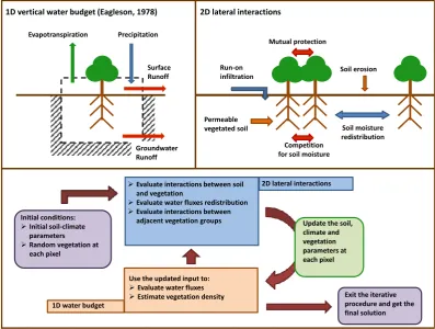
However, the aforementioned spatial configuration of veg-etation and water fluxes across the study hillslope is, a priori, unknown. In order to find it, that is, in order to determine the local-scale fluxes and vegetation density that are in equilib-rium with the hillslope-scale conditions, we use an iterative procedure. For a given set of initial climatic conditions and soil properties, long-term averages of annual fluxes of water and latent heat of evapotranspiration, as well as of vegeta-tion density, are estimated at the local scale for each one of the pixels of the study domain. Once the vertical fluxes and vegetal density are estimated at the local scale through the vertical water budget, the mutual lateral effects of vegetation and fluxes are evaluated. As mentioned before, those mutual effects are predicated on the assumption that vegetation and fluxes exert mutual feedback within the hillslope. Evaluation of lateral effects allows estimation of an updated set of in-puts (e.g., water input from uphill, feedback of soil moisture on albedo) and soil parameters (e.g., feedback of vegetation density on soil hydraulic conductivity) that are used to per-form the subsequent iteration. A flow chart of the simulation procedure is provided in Fig. 2.

Because the configuration of the local (i.e., at the pixel scale) water fluxes is obtained by redistributing the available global (i.e., of the entire domain) water input, the global wa-ter budget is actually satisfied at each step of the iwa-terative procedure. Analogous reasoning can be made with respect to the latent heat evapotranspiration flux.

3.2 1-D water budget: vertical fluxes and forcings

The water budget at any pixel of our study domain is quan-tified using a one-dimensional physically based mechanis-tic representation of soil moisture dynamics as forced by a stochastic climate (Eagleson, 1978a, b, c, d, e, f, g). It de-scribes the relationship between annual amounts of precip-itation, runoff (both surface and groundwater), infiltration and evapotranspiration as a function of volumetric soil mois-ture and soil and vegetation characteristics (additional details are provided in Appendix). In doing so, the model assumes that the soil–vegetation system is in a long-term equilibrium with climate, and that the value of long-term equilibrium soil moisture maximizes vegetal biomass and minimizes vege-tation stress (Eagleson, 1978f). It is indeed the assumption of long-term climate–soil–vegetation equilibrium that made Eagleson’s model our optimal choice for the characteriza-tion of the 1-D vertical dynamics. Although it can be argued that the short-term behavior of the biotic system is driven by short-term climatic forcings (e.g., few large pulses of pre-cipitation), the vegetation patterns we are interested in are observed across long time spans, suggesting that they are the result of a long-term adaptation process.

Eagleson’s water balance model characterizes the soil in terms of the following hydraulic parameters: total porosity, pore size distribution index, surface retention capacity, satu-rated hydraulic conductivity and satusatu-rated matric potential. The model describes the climate drivers as a function of: mean storm intensity, mean storm duration, mean time be-tween storms, rainy season length, mean and variance of storm depth, mean annual precipitation and mean annual potential evapotranspiration.

In Eagleson’s model, the role of vegetation in the water balance is captured through the plant transpiration efficiency,

kv, defined as the ratio between the potential rate of

transpira-tion to the potential rate of bare soil evaporatranspira-tion and through the fractional vegetation cover or vegetation density,M.

The output of the model is characterized by long-term av-erages of the water fluxes (i.e., evapotranspiration, surface runoff and groundwater runoff) as well as the long-term equi-librium soil moisture content and the vegetation density. The estimation of vegetation density and water fluxes is predi-cated on the assumption that the soil–vegetation system is in a long-term equilibrium with climate, and that the value of long-term equilibrium soil moisture maximizes vegetal biomass and minimizes vegetation stress (Eagleson, 1978f). The water balance model is summarized in Eqs. (1)–(22) of Eagleson (1978f).

3.3 2-D spatial feedbacks characterization: horizontal fluxes and interactions

Precipitation Evapotranspiration

Surface Runoff

Groundwater Runoff

Run-on infiltration

Mutual protection

Soil moisture redistribution Competition

for soil moisture

Soil erosion

Permeable vegetated soil

1D vertical water budget (Eagleson, 1978) 2D lateral interactions

Evaluate interactions between soil and vegetation

Evaluate water fluxes redistribution Evaluate interactions between

adjacent vegetation groups

Use the updated input to: Evaluate water fluxes Estimate vegetation density

Update the soil, climate and vegetation parameters at each pixel Initial conditions:

Initial soil-climate parameters Random vegetation at

each pixel

Exit the iterative procedure and get the final solution 2D lateral interactions

1D water budget

Fig. 2. Schematic of the 1-D vertical budget model and the 2-D lateral interactions with flowchart of the simulation procedure of the soil–

climate–vegetation system.

soil–vegetation system by perturbing the thermal and aero-dynamic properties of the canopy layer as well as the soil structure (i.e., texture, porosity, connectivity, hydraulic con-ductivity, etc.). These perturbations in turn lead to changes in the water and energy fluxes in the neighborhood of the plant that may promote or inhibit the establishment of surround-ing vegetation. We focus only on a subset of factors that we hypothesize are the main drivers of the process of vegeta-tion pattern formavegeta-tion and evoluvegeta-tion. These factors are: (1) modification of the spatial distribution of soil hydraulic con-ductivity by vegetation, (2) infiltration of surface runoff, a phenomenon known as run-on infiltration, (3) spatial recon-figuration of soil albedo, (4) spatial soil moisture redistribu-tion due to roots, and (5) redistriburedistribu-tion of nutrients.

Although fire, livestock, and other such external forces may be the main cause determining vegetation patterns in some instances, vegetation patterns as those shown in Fig. 1 are observed even in the absence of such forces. Therefore, our work focuses on the feedbacks and interactions between vegetation, soil, and hydro-climatic processes only.

3.3.1 Effect of vegetation on soil hydraulic conductivity

The soil hydraulic characteristics vary depending on the pres-ence or abspres-ence of vegetation and on the evolution of

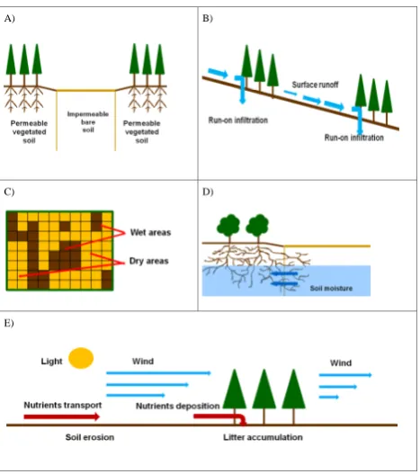
vege-tation density. Plants influence erosion and sediment trans-port by limiting the effect of wind and slowing the surface runoff velocity, therefore constituting areas of potential sedi-ment accumulation. In addition, the superficial soil of a veg-etated area is much richer in litter and organic debris, there-fore it is richer in nutrients and more porous and permeable. Permeability of deeper layers is also affected by the presence of roots and rotting roots, which create preferential routes for infiltrated water (Boaler and Hodge, 1962; Bromley et al., 1997). All of these effects have been observed in areas characterized by vegetation patterns, where vegetated soil ex-hibits higher permeability than adjacent bare soil, which of-ten has a highly impermeable superficial crust (Valentin et al., 1999). The range of hydraulic conductivity of an area characterized by vegetation patterns can be very wide, often spanning several orders of magnitude and subjected to ran-dom variations within very short distances (Bromley et al., 1997). Soil permeability at a site, therefore, is a function of vegetation density (see schematization in Fig. 3a).

We model the saturated hydraulic conductivity as a con-tinuous function of vegetation densityMXat the given point Xas follows:

KsX= i=10

X

i=1

A) B)

C) D)

E)

Fig. 3. Qualitative schematization of the interactions between soil,

climate and vegetation. (A) Effect of vegetation on soil permeabil-ity. (B) Effect of vegetation on run-on infiltration. (C) Effect of soil moisture on soil reflectance. (D) Effect of roots on soil moisture.

(E) Other spatial interactions (effect of vegetation on wind, light,

nutrients, etc.).

(1) whereI[α,β)(M)is the indicator function such that:

I[α,β)(M)=

 



1, α≤M < β

0, otherwise

.

(2)

The choice of the coefficientsai andbi of Eq. (1) is aimed at

obtaining a piecewise continuous function spanning a range of saturated hydraulic conductivity values compatible with observations as reported in the literature (Bromley et al., 1997) which, for the sites where vegetation patterns emerge, are typically found in the interval 10−6to 10−3cm s−1over a range of vegetation density ranging between 0 and 1. 3.3.2 Run-on infiltration of surface runoff

A non-uniform spatial distribution of hydraulic conductivity affects both the vertical water fluxes as well as the water in-put of downstream points through the process of run-on infil-tration. Surface runoff plays a key factor in the development of soil and vegetation. Part of the surface runoff can pond in small depressions or be trapped in areas of litter deposi-tion downhill and infiltrate (Bromley et al., 1997) (see also schematization in Fig. 3b). The amount of surface runoff that

Fig. 4. (A), (B), (C) Aerial photographs of natural patterns (Tiger

Bushes) in Niger (13◦200N, 2◦040E). (D), (E), (F) Digitized rep-resentation of the vegetation covers of the natural patterns corre-sponding respectively to (A), (B) and (C). (G), (H), (I) Simulated patterns.

infiltrates depends on many factors, such as soil properties, topography, overall water input, characteristics of the rain event and so on. The runoff produced accumulates along the hillslope, causing erosion and sediment transport.

Thus, the long-term water balance at each pointX consid-ers a water input,PX, given by the sum of the long-term av-erage precipitationmPA atXand the average surface runoff, RsY, coming from the uphill locationY:

PX=mPA+RsY, Y =X+ ∇FX·ds,

(3) whereFXis the topographic elevation function of the domain

evaluated at the pointXand∇is the gradient operator. 3.3.3 Effect of vegetation on albedo

and Asner, 2002; Wang et al., 2005). For soil–vegetation sys-tems, less absorbed net energy means less available energy for sensible heating and for evaporating water. Consequently, all else being equal, higher albedo corresponds to lower po-tential rate of evapotranspiration.

We express the total albedo,ρT, as an exponentially

de-creasing function of the long-term mean of soil moisture such that:

ρTX=ρT∗X−A·

h

e−s0X/B_−e−1/Bi_{, (4)} whereρ_T∗ is the total (i.e., all-frequency) surface albedo for saturated soil ands0X is the soil moisture, whileA andB

are coefficients whose value depends on the properties of the surface. This formulation accounts explicitly for the dence of albedo on soil moisture and implicitly for its depen-dence on vegetation through the dependepen-dence of soil moisture on vegetation density. For our simulations,ρ_T∗was set to 0.25,

Ato 0.11 andBto 0.3 (Lobell and Asner, 2002). 3.3.4 Soil moisture redistribution by roots

The root configuration is peculiar of each vegetation species and is affected by the plant’s age and health, as well as the soil characteristics, water availability, temperature, and other environmental factors. Developing a model of moisture re-distribution by roots that encodes all of these spatially and temporally varying effects is a complex task that goes be-yond the scope of this work. We propose a basic approach based on the simplifying assumption that the root character-istics of the vegetation populating the domain are spatially uniform and that soil moisture can be rerouted out of a pixel into another by root networks only if they extend across the pixel borders (Fig. 3d). We model the net exchange of water input,PX, at each point as:

dP dX _X

=ξR−1

4 ·

d(M·kv·P )

dX _X , (5)

wherekvrepresents the transpiration efficiency andξR

repre-sents the degree to which roots extend over the four adjacent pixels as the ratio of the rooted area to the characteristic area of the pixel:

ξR= Aroots

Acell

(6)

The parameterξR defines a range of root actions and allows

us to take into account the process of subsurface water trans-fer between adjacent pixels promoted by root systems.

Equation (5) implies that roots spreading across the bor-ders of a cell can uptake a fraction of the soil moisture of the neighboring cell in a way that is proportional (proportionality being given by the parameterξR)to the vegetation density of

the contiguous pixels and to their transpiration efficiencies.

3.3.5 Effect of vegetation on transpiration efficiency

The interactions between individual plants are multifold and may lead to positive and negative feedbacks on vegetation density. While, on the one hand, plants compete for water and nutrients through roots and for light through foliage (Barbier et al., 2008; Holmgren et al., 1997), they can also protect each other from extreme fluctuations of temperature and hu-midity, from the action of surface runoff, from mechanical or herbivore damages, and can improve soil properties through litter formation, augmented soil porosity and nutrient replen-ishment (Holmgren et al., 1997; Borgogno et al., 2009) (see also Fig. 3e).

In this study we express the cumulative effect of those in-teractions as a function of their impact on the transpiration ef-ficiency,kv, following the reasoning that the net result of fa-cilitation/competition should be to improve/worsen water use efficiency by increasing/decreasing the quantity of biomass that can be produced out of a certain amount of transpired water.

Therefore, we model the transpiration efficiency,kvX, at a

certain pointX, as a function of: a base value for the tran-spiration efficiency,kv; the local vegetation density,MX; the

vegetation density of surrounding points,MU,MD,ML,MR,

the hillslope-scale vegetation density at the initial time step,

M; the local surface runoff,RsX; the surface runoff of

imme-diately upslope and downslope,RsU,RsD; and the

hillslope-scale average surface runoff for uniform vegetation density at the initial step,Rs. This function has the following form: kvX=max0.5,min1, kv+(1kvX)1+(1kvX)2

+ +(1kvX)31kvX

4+(1kvX)5

, (7)

where:

(1kvX)1= −α1·

MX−M

M (8)

(1kvX)2= −α2·

MU+MD+ML+MR−4·M

M , where           

U=X+ ∇FX·ds D=X− ∇FX·ds L=X+2X·ds R=X−2X·ds

where2X⊥∇F

(9)

(1kvX)3= −α3·

Rs−RsX mPA

(10)

(1kvX)4= −α4·

RsU−RsX mPA

,whereU=X+ ∇FX·ds (11)

(1kvX)5=α5·

RsD−RsX mPA

Equations (8) and (9) describe the change of the local tran-spiration efficiency at pointXas a function of the vegetation density at both the point itself and at the adjacent ones. The presence of the negative sign in Eqs. (8) and (9) derives from the fact that the presence of vegetation in the given pixel and in its neighborhoods is assumed to produce a facilitation ef-fect for further establishment of vegetation.

Equations (10), (11) and (12), on the other hand, reflect the effect of surface runoff through the processes of erosion and sedimentation of both soil particles and nutrients. The negative sign in Eqs. (10) and (11) are suggested by the fol-lowing considerations: (1) when a given location (i.e., pixel) is subjected to a surface runoff,RsX, larger than the average

surface runoff corresponding to uniform density,Rs, it is

con-currently subjected to soil erosion and nutrients deprivation; (2) when a given pixel is subjected to a surface runoff,RsX,

lower than the surface runoff of the upstream pixel,RsU, it

benefits from the partial deposition of incoming soil particles and nutrients and (3) when a given pixel is subjected to a sur-face runoff,RsX, lower than the downstream pixel,RsU, it is

subjected to an accelerated superficial flow which exposes it to nutrients and soil loss.

4 Simulation of the system

The climate–soil–vegetation system was simulated under various combinations of climatic forcing, soil parameters and lateral interaction functions (Eqs. 8 through 12) in order to explore the conditions controlling the mechanism of pattern emergence and evolution. We present results of the simula-tion of the system on a study domain of 50x50 pixels, repre-senting a hillslope of about 105m2. Boundary conditions of the system are: (1) for all domain borders, fractional vegeta-tion coverage is kept equal to the initial uniform soluvegeta-tion (ob-tained by using the domain-averaged inputs and equal to the vegetal density of each pixel at the preliminary step of simu-lation); (2) for upstream and lateral borders, water fluxes are kept equal to the initial uniform solution; and (3) free flow condition for the downstream boundary, allowing complete drainage downhill.

We used the model both to simulate real sites character-ized by the presence of vegetation patterns and for a non site-specific system (the latter in order to evaluate the system sensitivities to each mechanism considered.) Unless other-wise stated, simulations were carried out on a constant slope domain whose hydraulic properties and climatic forcing are reported in the “base conditions” column of Table 1. In order to incorporate the typical random spatial variability of soil conductivity (Bromley et al., 1997), a random component is superimposed to the value ofKsX(n)obtained with Eq. (1).

5 Results and discussion

5.1 Spatial analysis

In order to compare different typologies of patterns and ob-jectively measure the individual impact of the climatic and hydraulic properties of the system on pattern emergence and characteristics, we explore the following spatial characteris-tics of vegetation fields:

– Probability density functions (PDFs) and conditional PDFs of vegetation density at the pixel level.

– Power spectral density functions of the vegetation den-sity fields.

– Number, size and shape of vegetation clusters.

5.1.1 PDFs and conditional PDFs of vegetation density

PDFs of the vegetation density at the pixel scale can be used to evaluate how different a given vegetation field is from the typical field that would be produced if the plants were dis-tributed randomly and independently in space. In this case, we may assume that the vegetation density of each pixel is a one to one function of the number of plants present within the pixel itself. Following this assumption, the PDF of the pixel vegetation density throughout the domain would be normally distributed with mean equal to the average pixel vegetation coverage1. For self-organized vegetation patterns, the pres-ence of a clump of vegetation at a certain point in space has an impact on the vegetation establishment in its neighbor-hood. Therefore, presence of self-organized structures can be inferred from the analysis of conditional PDFs of the vege-tation density. We do so by evaluating the PDF of vegevege-tation density for all those pixels having at least one neighbor char-acterized by vegetation density higher than the overall do-main average. The same conditioning is done on the neigh-borhood of a pixel characterized by vegetation density lower than the domain average. In order to detect spatial anisotropy, conditional PDFs are evaluated for the x-direction (by look-ing at the vegetation density of the two adjacent pixels in the x-direction), for the y-direction, and for all directions. The analysis of the conditional PDFs along the two orthog-onal directions provides a useful metric to investigate spatial anisotropy. For example, the x-direction PDF conditional on neighbors having larger than average density investigates the correlation between vegetation groups and their neighbors along the x-axis; if the x-direction conditional PDF is shifted towards larger densities when compared to both the overall PDF and the y-direction conditional PDF, it is evidence that vegetated patches tend to extend along the x-direction.

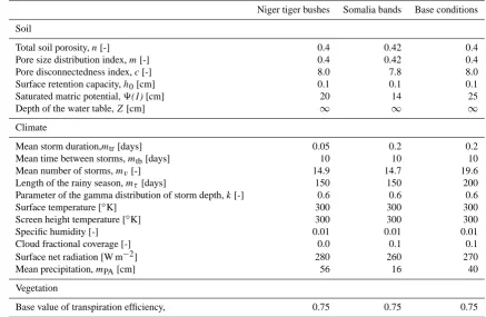
Table 1. Climate, soil and vegetation properties of the system.

Niger tiger bushes Somalia bands Base conditions

Soil

Total soil porosity,n[-] 0.4 0.42 0.4

Pore size distribution index,m[-] 0.4 0.42 0.4

Pore disconnectedness index,c[-] 8.0 7.8 8.0

Surface retention capacity,h0[cm] 0.1 0.1 0.1

Saturated matric potential,9(1) [cm] 20 14 25

Depth of the water table,Z[cm] ∞ ∞ ∞

Climate

Mean storm duration,mtr[days] 0.05 0.2 0.2

Mean time between storms,mtb[days] 10 10 10

Mean number of storms,mv[-] 14.9 14.7 19.6

Length of the rainy season,mτ[days] 150 150 200

Parameter of the gamma distribution of storm depth,k[-] 0.6 0.6 0.6

Surface temperature [◦K] 300 300 300

Screen height temperature [◦K] 300 300 300

Specific humidity [-] 0.01 0.01 0.01

Cloud fractional coverage [-] 0.0 0.1 0.1

Surface net radiation [W m−2] 280 260 270

Mean precipitation,mPA[cm] 56 16 40

Vegetation

Base value of transpiration efficiency, 0.75 0.75 0.75

5.1.2 Analysis of vegetation clusters

We arbitrarily define a cluster of vegetation as a group of ad-jacent pixels characterized by vegetation density larger than the domain average density. In defining a cluster, only those pixels in the von Neumann neighborhood of any given pixel are considered. For each cluster defined as above, we cal-culate the size,Si, (that is, the number of pixels that

com-pose theith cluster), the span along the x- and y-directions, the shape ratio (as the ratio between the span along the x-direction and the span along the y-x-direction) and the fraction of area filled (as the ratio between the cluster size and the product between the span along the two directions). We also calculate the total number of clusters present in the whole domain.

This definition of clusters allows us to compare observed and simulated vegetation clumps with the clumps resulting from a homogeneous binomial process with probabilityp

such that:

p=

NCLUSTERS

P

i=1 Si

SizeDOMAIN

. (13)

We arbitrarily define a vegetation pattern as a clustered con-figuration whose average cluster size is higher than the 0.975 quantile of the cluster size distribution of the correspond-ing (through thepfound in Eq. 13) uniform binomial

pro-cess. In addition, based on the statistical characteristics of the clumps of vegetation, we distinguish three types of pat-tern as follows:

– Spots: a pattern whose shape ratio is within the range 0.6–1.6.

– Bands: a pattern whose shape ratio is lower than 0.6 or higher than 1.6.

– Labyrinths: a pattern whose largest cluster is embedded in a rectangular area of at least 75 % of the domain and whose fraction of area filled is less than 0.75.

This classification implies that spots are structures whose di-mensions in the x- and y-directions are similar (and, thus, characterized by shape ratios close to 1), while bands are characterized by having a dominant dimension (either on x or y). Labyrinthine patterns, on the other hand, are charac-terized by a few big clumps of vegetation (thus the reason why we look at the areal span of the largest cluster) embed-ding several patches or stripes of bare soil (thus the reason why we look at the area of the cluster effectively filled with vegetation).

5.2 Simulated patterns versus natural patterns

African locations, namely an area of Niger near Niamey and a region of Somalia near Garoowe.

5.2.1 Niger

The area situated about 45 km south of Niamey, the capital of Niger, is known for the characteristic vegetation patterns known as tiger bushes. The average annual precipitation of the region is 56 cm, half of which falls at an intensity higher than 35 mm h−1and a third above 50 mm h−1 (Bromley et al., 1997). Soil is gravelly sandy loam and is highly prone to crusting in bare areas, while vegetation is concentrated in stripes of a few tens of meters wide and a few hundred meters long (Bromley et al., 1997).

The model parameters for these simulations correspond to the climatic and hydraulic characteristics of the area reported in the above literature and are shown in Table 1 (values of temperature, specific humidity and cloud coverage in the ta-ble were arbitrarily assigned in order to match the observed value of potential evapotranspiration). In addition, soil hy-draulic conductivity at each pixel was calculated as a func-tion of the vegetafunc-tion density at that pixel and was set to span a range of 3×10−7to 9.5×10−6m s−1for the crusted bare soil and a full canopy coverage, as suggested by field measurement (Bromley et al., 1997) and estimations from grain analysis (Casenave and Valentin, 1992). Values for the parameters of Eq. (4) through Eq. (12) are provided in Ta-ble 2. Since the above literature does not provide enough in-formation for the estimation of all the parameters listed in the table, the remaining parameters (in particular the ones of Eq. 8–12) values were chosen within ecologically reasonable bounds (see Sect. 3.3.5) to tune the model output in order to qualitatively match the observations.

Google Earth aerial photographs of this region of Niger were used to infer field observations. A few random study areas were sampled from the vast region characterized by the presence of tiger bushes, all of which have a surface area of about 105 square meters (see Fig. 4). The vegetation den-sity at every pixel was estimated from the gray color levels of the digitized picture pixels mapped to the intervalM=0 for those pixels characterized by bare soil, andM=1 for those characterized by full coverage. Photos, whose original resolution was of about 400×400 pixels, were then further processed in order to match the resolution of our study grid. This was done by superimposing our study grid on the orig-inal photo and averaging the fractional coverage of the set of pixels of the original photo that fell within the bounds of each pixel of our 50×50 grid.

An initial qualitative comparison between simulations and observations is presented in Fig. 4, where three original aerial photos are shown together with their digitized vegetation density maps and three sample results from our simulations. The figure shows a good qualitative agreement between nat-ural and simulated patterns in terms of typical shape and

di-mension of the vegetation structures and in the overall spatial configuration of the patterns within the study domain.

Results of several simulations exhibited a noteworthy sen-sitivity of the emerging patterns to changes in the spatial in-teraction functions and in particular to the dependence ofkv

(Eq. 9) and hydraulic conductivity on vegetation (Eq. 1). Dif-ferences between patterns in Fig. 4g and f, for example, are due to changes of about 5% in the coefficients of the Eq. (9); Fig. 4h was obtained by increasing the soil conductivity in the interval corresponding to a fractional cover only in the range of 0.3 to 0.5 by about 10 %, keeping the overall span of the range fixed between 3×10−7 to 9.5×10−6m s−1. The above considerations suggest that the combination of the mechanisms of run-on infiltration (mainly driven by plant feedback on soil conductivity) and facilitation (due to plants’ improved efficiency in water use) is extremely important not only for the formation of patterns in the study area, but also for their shape and dimension. Thus, given that the global (i.e., climatic) conditions are favorable to pattern formation, the peculiar patterning is driven by the local feedbacks.

An analysis of the spatial distribution of water fluxes and soil moisture content is provided in Fig. 5. In particular, Fig. 5a shows the value of the average effective input at each pixel, computed as average precipitation plus the run-on and adjusted to account for the effect of roots as in Eq. (5). As shown, many areas receive an amount of water several times higher than the actual mean precipitation from the low per-meable pixels located upstream, in accordance with field ob-servation of concentration factors (ratio between the effec-tive amount of water received and the actual precipitation) as high as 3 and 4 (Bromley et al., 1997). In addition, the higher values of groundwater runoff observable in correspon-dence of the vegetated patches (shown in Fig. 5b) confirm that vegetation favors the infiltration of the hillslope run-on. Taken together, the extra water input from upstream and the enhanced permeability of the more vegetated soil trigger a positive feedback for further vegetal biomass establishment, confirming that surface water redistribution due to infiltra-tion of run-on is one of the main drivers of pattern formainfiltra-tion, (Boaler and Hodge, 1962; Valentin et al., 1999; Casenave and Valentin, 1992). The latter result will be further investi-gated later in the paper. In accordance with published results (Borgogno et al., 2009), our simulation shows that the aver-age soil moisture content is higher in the areas under vege-tated patches (especially in their uphill side) than in the sur-rounding bare soil (Fig. 5c); this, in turn, creates suitable conditions for the sustainment and/or further development of vegetation.

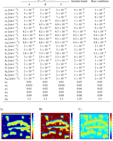
Table 2. Model parameters.

Niger tiger bushes

Somalia bands Base conditions

A B C

a1[cm s−1] 3×10−5 3×10−5 3×10−5 9×10−6 2×10−5 a2[cm s−1] 5×10−5 5×10−5 5×10−5 1×10−5 4×10−5 a3[cm s−1] 8×10−5 7×10−5 7×10−5 3×10−5 8×10−5 a₄[cm s−1] 3×10−4 4×10−4 4.5×10−4 1×10−4 3×10−4

a5[cm s−1] 6×10−4 6.5×10−4 6.8×10−4 7×10−4 8×10−4 a6[cm s−1] 8×10−4 8×10−4 8.5×10−4 9×10−4 9×10−4 a7[cm s−1] 8.2×10−4 8.2×10−4 8.7×10−4 9.1×10−4 9.2×10−4 a8[cm s−1] 8.4×10−4 8.4×10−4 8.9×10−4 9.2×10−4 9.4×10−4 a9[cm s−1] 8.6×10−4 8.6×10−4 9.1×10−4 9.3×10−4 9.6×10−4 a10[cm s−1] 8.8×10−4 8.8×10−4 9.3×10−4 9.4×10−4 9.8×10−4 b1[cm s−1] 2×10−4 2×10−4 2×10−4 1×10−5 2×10−4 b2[cm s−1] 3×10−4 2×10−4 2×10−4 2×10−4 4×10−4 b3[cm s−1] 2.8×10−3 3.3×10−3 3.8×10−3 7×10−4 2.2×10−3 b4[cm s−1] 3×10−3 2.5×10−3 2.3×10−3 6×10−3 5×10−3 b5[cm s−1] 2×10−4 1.5×10−3 1.7×10−3 2×10−3 1×10−3 b6[cm s−1] 2×10−4 2×10−4 2×10−4 1×10−4 2×10−4 b7[cm s−1] 2×10−4 2×10−4 2×10−4 1×10−4 2×10−4 b8[cm s−1] 2×10−4 2×10−4 2×10−4 1×10−4 2×10−4 b9[cm s−1] 2×10−4 2×10−4 2×10−4 1×10−4 2×10−4 b10[cm s−1] 2×10−4 2×10−4 2×10−4 1×10−4 2×10−4

α1 0.01 0.01 0.01 0.03 0.01

α2 0.019 0.02 0.018 0.05 0.02

α3 0.03 0.03 0.03 0.04 0.03

α4 0.03 0.03 0.03 0.04 0.03

α5 0.09 0.09 0.09 0.08 0.09

ξR 1.5 1.5 1.5 1.25 1.5

Fig. 5. (A) Ratio between the effective amount of water received and annual precipitation for the simulated pattern in Fig. 4g. (B) Long-term

groundwater runoff on the study domain for the simulated pattern in Fig. 4g. (C) Long-term soil moisture content during the rainy season on the study domain for the simulated pattern in Fig. 4g.

higher than the domain average. The latter suggests that the vegetal density of each pixel is more likely to be higher than the average, providing that it is in the neighborhood of a pixel whose cover is also higher than the spatial aver-age. The opposite is true when the condition is on the neigh-bor pixel having a density that is lower than the average. A slight prevalence of structures in the x-direction (perpendic-ular to the domain slope) is apparent from the analysis of the

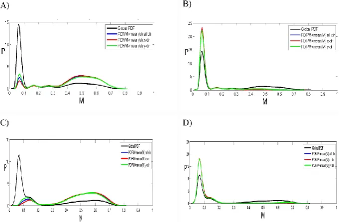
Fig. 6. Global and conditioned PDF analysis of the Niger patterns. Panels (A/B): natural, and (C/D): simulated vegetation; panels (A/C):

density higher than global average, and (B/D): density lower than global average. (A) PDFs of vegetation density for the natural pattern shown in Fig. 4a (as digitized in Fig. 4d): global PDF (black line) and PDFs of vegetation density conditioned on having a neighbor pixel with vegetation density higher than the global average for all directions (blue line), x-direction (red line) and y-direction (green line). (B) PDFs of vegetation density for the natural pattern shown in Fig. 4a (as digitized in Fig. 4d): global PDF (black line) and PDFs of vegetation density conditioned on having a neighbor pixel with vegetation density lower than the global average for all directions (blue line), x-direction (red line) and y-direction (green line). (C) PDFs of vegetation density for the simulated pattern shown in Fig. 4g: global PDF (black line) and PDFs of vegetation density conditioned on having a neighbor pixel with vegetation density higher than the global average for all directions (blue line), x-direction (red line) and y-direction (green line). (D) PDFs of vegetation density for the simulated pattern shown in Fig. 4g: global PDF (black line) and PDFs of vegetation density conditioned on having a neighbor pixel with vegetation density lower than the global average for all directions (blue line), x-direction (red line) and y-direction (green line).

Fig. 7. Power spectral densities of the vegetation density field;

fre-quencies (in the horizontal axis) are expressed in terms of number of wavelengths present within the domain length and width. (A) Average of the 1-D power spectral densities of the vegetation den-sity for the natural pattern shown in Fig. 4a along the x-direction (black line) and y-direction (red line). (B) Average of the 1-D power spectral densities of the vegetation density for the simulated pattern shown in Fig. 4g along the x-direction (black line) and y-direction (red line).

PDF. Conversely, for the same interval of fractional cover-age, higher density is shown for the PDF of the vegetal den-sity of pixels being in the x-direction neighborhood of a pixel with vegetal density lower than the domain average.

Fig. 8. (A) Aerial photograph of a natural vegetation pattern in

So-malia (7◦430N, 48◦020E); (B) Digitized representation of the veg-etation cover of the natural pattern in (A). (C) Sample simulated pattern.

by detecting a prevalence of structures recurring at frequen-cies between 2 and 6 (that is, 2 to 6 structures per domain length) along the y-direction.

The analyses of the characteristics of the vegetation clus-ters of both natural and simulated vegetation fields, whose results are reported in Table 3, show that two out of three natural patterns (Fig. 4d and e) fall within our definition of spots, while the pattern in Fig. 4f is labyrinthine. Simulated patterns, however, are all spotted, even though the one shown in Fig. 4i, whose largest cluster covers the 68 % of the do-main, almost meets the requirement for being classified as labyrinthine.

5.2.2 Somalia

Vegetation stripes are a widespread occurrence on the So-maliland plateau (Boaler and Hodge, 1962) and in the Punt-land area (Borgogno et al., 2009). The area is semi-desert and characterized by an arid climate with precipitation highly variable in space and time (Muchiri, 2007). The area selected is located about 30 km west of Garoowe, the administrative capital of the Puntland region of Somalia and is characterized by annual precipitation ranging between 10 and 20 cm yr−1, mostly occurring in the period of May–September (Muchiri, 2007). Dominant soils are Gypsisol and Calcisol (Venema, 2007), according to the FAO definition, and are characterized by hydraulic conductivity that can be as low as a few cm/day, but can span two orders of magnitude. These kinds of soil are also very susceptible to crusting and cracking (Driessen et al., 2001).

A study area of about 5×105m2, located at 7◦₄₃0_N, 48◦₀₂0_{E and characterized by the presence of vegetation} stripes was selected from the Puntland area near Garoowe. In comparison to the Niger case, the climate is drier (pre-cipitation being less than one third that of the Niger case) and patterns – in this case well-defined stripes – occur at a slightly larger scale. In accordance with the climatic and soil information reported above, the simulations of the area used the parameters shown in Tables 1 and 2. Results of the simu-lations were compared to the observed patterns, as shown in Fig. 8 through Fig. 10.

As done for the case of the Niger tiger bushes, a sam-ple aerial photograph was processed in order to obtain es-timates of the vegetal density at a 50×50 study grid, and compared with the simulated results (Fig. 8). The comparison shows a good qualitative match between observed and sim-ulated vegetal spatial configurations. Dimensions and shape of the bands and of the inter-band gaps are similar, although the vegetation structures emerging from the simulations look slightly sharper than the observed ones. In addition, orien-tation of the bands perpendicular to the slope is clearer in the simulations than in the observations. This is because, al-though the direction of the natural and simulated slope was set to coincide, the natural topography presented some ir-regularities, and the simulations were performed on a

reg-ular slope. Nevertheless, both in the observed and simulated case, the configuration of vegetal density is characterized by stripes of vegetation a few tens of meters wide downslope from and extending across the entire study domain.

Compared to the previously analyzed case of the Niger tiger bushes, the directionality of the Somaliland plateau veg-etation patterns is more noticeable, both in the observations and in the simulations. Moreover, the total amount of vegeta-tion (integrated across the domain) is smaller than in the case of the Niger tiger bushes, as easily noticeable from the com-parison of the PDFs of the vegetal density shown in Figs. 6 and 9. Analysis of the PDFs in Fig. 9 also shows that the presence of multiple modes is less evident here than in the case of the Niger tiger bushes, when the unconditioned PDF of the vegetation density is considered. However, multiple modes become apparent in the conditional PDFs of both the observed and the simulated vegetation fields, especially with respect to the PDF in the x-direction conditioned on neighbor density higher than the domain average. As observed in the case of the Niger patterns, the presence of multiple modes in the conditional PDFs and, in general, the fact that the condi-tional PDFs look different than the uncondicondi-tional PDF, im-plies that the vegetation at a given pixel has an impact on the vegetation distribution of its neighborhood. In particu-lar, the probability of finding a pixel whose fractional cover-age is higher than the avercover-age is greater in a neighborhood of pixels that are themselves characterized by above-average density, supporting the observation that vegetation tends to form clumps rather than being distributed completely ran-domly in space. In addition, the PDF conditioned on x-direction neighbor density higher than the domain average, shows higher density for values of vegetation in the upper end of the domain interval than the other (conditional and unconditional) PDFs; this confirms the prevalence of stripes of vegetation in the x-direction itself, that is, perpendicular to the domain slope.

Spectral analysis (Fig. 10) supports the conclusions drawn from both the qualitative analysis and the analysis of the PDFs of the vegetation density, showing the presence of fre-quencies between 5 and 10 cycles along the domain only along one direction. However, comparisons between the spectral densities of the observed and simulated vegetation field also imply that the prevalence of stripes perpendicular to the main slope is higher in the simulated field than the ob-served. Since the only anisotropic effect present in our model is topographic (through the surface runoff production and run-on infiltration), and the shape of the natural pattern seems to indicate that the governing mechanism of pattern forma-tion is topographic and gravitaforma-tional, we attribute the dis-crepancy between observations and simulations to the irreg-ularities of the natural topography of the observed area with respect to the regular slope used in the simulated domain.

Table 3. Cluster analysis for natural and simulated patterns in Niger and Somalia.

Niger Somalia

Natural Simulated Natural Simulated

Figure 4d 4e 4f 4g 4h 4i 15b 15c

Number of clusters 21 20 29 22 30 14 49 24

Average cluster size 42 38 38 37 32 90 15 28

Range 0.025–0.975 quantile of cluster size for binomial process

[1–18] [1–12] [1–35] [1–14] [1–24] [1–74] [1–12] [1–9]

Shape ratio 1.4 1.5 1.1 1.2 1.4 1.2 1.9 2.6

Percentage of domain filled by the largest cluster

0.35 0.34 0.78 0.57 0.18 0.68 0.36 0.15

Fraction of area of the largest cluster filled with vegetation

0.51 0.35 0.37 0.42 0.63 0.44 0.21 0.23

Cluster type Spots Spots Labyr Spots Spots Spots Bands Bands

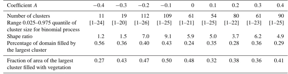
Table 4. Statistical analysis of the vegetation clusters for the fields of vegetation obtained with hydraulic conductivity functions, modified

from the base conditions through Eq. (14).

CoefficientA −0.4 −0.3 −0.2 −0.1 0 0.1 0.2 0.3 0.4

Number of clusters 11 19 112 109 61 54 80 61 90

Range 0.025–0.975 quantile of cluster size for binomial process

[1–24] [1–20] [1–26] [1–25] [1–21] [1–25] [1–22] [1–23] [1–25]

Shape ratio 1.2 1.5 7.0 9.1 5.9 5.0 3.7 6.2 4.9

Percentage of domain filled by the largest cluster

0.56 0.36 0.40 0.43 0.24 0.35 0.28 0.36 0.29

Fraction of area of the largest cluster filled with vegetation

0.27 0.43 0.47 0.50 0.48 0.32 0.38 0.36 0.41

5.3 Analysis of the hypothesized pattern-promoting dynamics

5.3.1 Impact of climate forcings

In order to explore the effect of the climate forcing on pat-tern formation and spatial characteristics of the vegetation distribution, the system was simulated by varying the cli-matic forcing, while keeping everything else fixed. All the inputs for these simulations are reported in the column titled “base conditions” of Tables 1 and 2. The soil–climatic condi-tions referred to here as base condicondi-tions are arbitrary and not representative of a specific site. We investigated the impact of two climatic components: mean annual precipitation and mean annual net radiation (through the impact that the latter has on potential rates of evapotranspiration).

Simulations showed that the shape and the presence of pat-terns at the hillslope scale depend not only on the mean an-nual precipitation but also on the characteristics of the rainy events (mean storm duration, mean time between storms, mean storm intensity, etc.). Below, we focus our analysis only on the dependence on the mean annual precipitation.

Figure 11 shows the result of the statistical analysis of the vegetation fields obtained for a range of mean annual pre-cipitation of 26 to 85 cm (the range was selected to be wide enough to detect the transition from bare hillslope to patterns and to densely vegetated hillslope without patterns).The vari-ation in mean annual precipitvari-ation was achieved by varying the mean storm duration only and leaving the mean storm intensity unchanged. All the other parameters of the model, both climatic and hydraulic, were kept at the values set for the “base conditions”. Figure 11a shows that patterns of veg-etation start to emerge for mean annual precipitation higher than 32 cm and that cease to exist when mean precipitation approaches 60 cm per year. Nearly all the patterned fields are banded, as shown in Fig. 11b, and none presents labyrinthine characteristics, as shown in Fig. 11c and d. Three sample fields obtained for annual precipitation of 70, 48 and 32 cm per year are presented in Fig. 12 for a visual interpreta-tion of the transiinterpreta-tion from undistinguishable patterns to self-organized structures.

Fig. 9. Global and conditioned PDF analysis of the Somalia patterns. Panels (A/B): natural, and (C/D): simulated vegetation; panels (A/C):

density higher than global average, and (B/D): density lower than global average. (A) PDFs of vegetation density for the natural pattern shown in Fig. 8a (as digitized in Fig. 8b): global PDF (black line) and PDFs of vegetation density conditioned on having a neighbor pixel with vegetation density higher than the global average for all directions (blue line), x-direction (red line) and y-direction (green line). (B) PDFs of vegetation density for the natural pattern shown in Fig. 8a (as digitized in Fig. 8b): global PDF (black line) and PDFs of vegetation density conditioned on having a neighbor pixel with vegetation density lower than the global average for all directions (blue line), x-direction (red line) and y-direction (green line). (C) PDFs of vegetation density for the simulated pattern shown in Fig. 8c: global PDF (black line) and PDFs of vegetation density conditioned on having a neighbor pixel with vegetation density higher than the global average for all directions (blue line), x-direction (red line) and y-direction (green line). (D) PDFs of vegetation density for the simulated pattern shown in Fig. 8a: global PDF (black line) and PDFs of vegetation density conditioned on having a neighbor pixel with vegetation density lower than the global average for all directions (blue line), x-direction (red line) and y-direction (green line).

Fig. 10. Power spectral densities of the vegetation density field;

fre-quencies (in the horizontal axis) are expressed in terms of num-ber of wavelengths present within the domain length and width.

(A) Average of the 1-D power spectral densities of the vegetation

density for the natural pattern shown in Fig. 4a along the x-direction (black line) and y-direction (red line). (B) Average of the 1-D power spectral densities of the vegetation density for the simulated pattern shown in Fig. 8c along the x-direction (black line) and y-direction (red line).

climatic conditions become more arid, clumps of vegetation decrease in number and increase in average size.

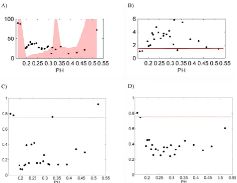
Fig. 11. Statistical analysis of the vegetation clusters for the fields

of vegetation obtained by varying annual precipitation. (A) Mean size of clusters and range 0.025–0.975 quantile of the mean cluster size corresponding to a binomial process with the same percent-age cover. (B) Mean ratio between the span in the x-direction and the span in the y-direction of each cluster; red line represents the boundary between spots and bands. (C) Percentage of the domain filled by the largest cluster; red line represents the minimum fraction of area filled for the field to be considered labyrinthine. (D) Fraction of area of the largest cluster filled by vegetation; red line represents the maximum fraction of the largest cluster that can be filled for the field to be considered labyrinthine.

Fig. 12. Effect of precipitation on pattern formation. (A) P = 32 cm yr−1; (B)P=48 cm yr−1; (C)P=70 cm yr−1.

enough to support a substantial amount of vegetation even in the absence of surface water redistribution or mechanisms of facilitation/competition. When this occurs, the impact of those dynamics of surface water redistribution and facilita-tion/competition becomes comparatively less important (that is, the lateral interactions are overpowered by the vertical wa-ter and energy fluxes) and does not induce the emergence of recognizable patterns. As the conditions become more arid, that is, for lower PH values (in our simulations for 0.2<PH<0.3), the water input from lateral redistribution becomes determinant for the amount of vegetation that es-tablishes at each pixel; moreover, the benefits of the facil-itation mechanisms that exist in the neighborhood of veg-etated pixels become (comparatively to more humid condi-tions) more significant and, thus, promote vegetation rear-rangement and pattern formation. For the lowest PH values,

Fig. 13. Statistical analysis of the vegetation clusters for the fields

of vegetation obtained by varying average net radiation. (A) Mean size of clusters and range 0.025–0.975 quantile of the mean cluster size corresponding to a binomial process with the same percent-age cover. (B) Mean ratio between the span in the x-direction and the span in the y-direction of each cluster; red line represents the boundary between spots and bands. (C) Percentage of the domain filled by the largest cluster; red line represents the minimum fraction of area filled for the field to be considered labyrinthine. (D) Fraction of area of the largest cluster filled by vegetation; red line represents the maximum fraction of the largest cluster that can be filled for the field to be considered labyrinthine.

Fig. 14. Effect of net radiation on pattern formation. (A) Net

radia-tion=210 W m−2; (B) Net radiation=250 W m−2; (C) Net radia-tion=290 W m−2.

that is, for the most arid conditions explored in this analysis, the climate conditions are so adverse to vegetation establish-ment that the study hillslope tends to be too scarcely vege-tated for the facilitation/competition dynamics to take place, ultimately resulting in the absence of patterns.

5.3.2 Temporal dynamics

Fig. 15. Statistical analysis of the vegetation clusters for the fields

of vegetation as a function of the ratio between annual precipita-tion and annual potential evapotranspiraprecipita-tion. (A) Mean size of clus-ters and range 0.025–0.975 quantile of the mean cluster size cor-responding to a binomial process with the same percentage cover.

(B) Mean ratio between the span in the x-direction and the span

in the y-direction of each cluster; red line represents the boundary between spots and bands. (C) Percentage of the domain filled by the largest cluster; red line represents the minimum fraction of area filled for the field to be considered labyrinthine. (D) Fraction of area of the largest cluster filled by vegetation; red line represents the maximum fraction of the largest cluster that can be filled for the field to be considered labyrinthine.

vegetal density at each pixel can either remain fixed (or not change significantly in between simulation steps), or it can undergo changes that – although significant at the pixel level – do not alter the macroscopic structure of the pattern itself, as in the case of vegetation structures that migrate across the domain.

In order to analyze this effect, we tracked the evolution of the vegetation field corresponding to the base conditions through different iteration steps, as shown in Fig. 16. The fig-ure shows the vegetation field at the 45th, 50th, 55th and 60th iteration step of our simulation procedure on a domain sloped from top to bottom in the figure. In this regard, we emphasize the fact that slope is only included to determine the direction of the surface run-on, as outlined in Eq. (3). It is evident that the patterns have already been established by the 45th step of the iteration, shown in Fig. 16a, and that the stripes mi-grate uphill as the simulation progresses. In addition to the migration, we notice that most bands are convex downslope, in accordance with many observations (Worral, 1959). As re-ported in the cited literature, pattern migration is induced by the effect of surface run-on ponding and infiltration in the uphill part of the stripes, which in turn creates a favorable opportunity for uphill expansion or migration of the vegeta-tion. This claim is supported by the analysis of the spatial distribution of soil moisture and water fluxes (not shown),

confirming the presence of wetter soils and higher infiltra-tion in the uphill porinfiltra-tion of the vegetainfiltra-tion bands, which as the simulation progresses, creates a favorable environment for further vegetation establishment and a positive feedback for the uphill expansion of the vegetation clumps. The drier conditions observed in the downhill portion of the bands, cre-ated by the fact that most of the available run-on has already infiltrated, result in the creation of adverse conditions that inhibit vegetation establishment.

However, a pattern migration was not observed in all the simulated cases. Several simulations (not shown) developed patterns that, once established, did not exhibit any tendency to migrate from their original location. This is attributed to the predominance of the local inhibition dynamics present in the uphill portion of vegetation clusters. In those cases, in fact, it has been observed for the pixels immediately up-hill of a clump of vegetation that the inhibition effect, due to the terms in Eqs. (10) and (11) (which reflect the effect of soil erosion due to the surface runoff), overpower the facilita-tion due to the presence of vegetafacilita-tion immediately downhill. In the real world, the strength of those inhibiting/facilitating factors would be determined by: overland flow velocity, soil texture, nutrients content, amount of litter produced by the vegetation, characteristics of the vegetation crown its impact on light exposure, etc. All those factors are not explicitly taken into account here, but are implicitly considered in the magnitude of coefficients in Eq. (8) through Eq. (11) and in their relative strength with respect to the processes directly impacting the water fluxes.

5.3.3 Impact of hydraulic conductivity

Regions where vegetation patterns occur are characterized by soils whose permeability is highly variable in space, being higher in areas of vegetated soil and lower where the soil is bare (HilleRisLambers et al., 2001; Bromley et al., 1997; Valentin et al., 1999; Boaler and Hodge, 1962; Saco et al., 2007). We account for the effect of plants on the permeability of the soil by expressing hydraulic conductivity as a function of vegetation density. In order to explore the impact that a vegetation-dependent hydraulic conductivity has on pattern formation, we consider the following three cases: (1) hy-draulic conductivity determined at each pixel as a function of vegetation according to Eq. (1) (base conditions); (2) spa-tially uniform hydraulic conductivity equal to the spatial av-erage corresponding to the base conditions; and (3) hydraulic conductivity at each pixel, randomly sampled from a uni-form distribution spanning the same range of hydraulic con-ductivities as in the base conditions. The first case encodes the vegetation-hydraulic conductivity feedback, the last two cases do not.

Fig. 16. Pattern migration. The evolution of a pattern is tracked through iteration steps (use red lines as reference): (A) 45; (B) 50; (C) 55; (D) 60.

Fig. 17. Effect of hydraulic conductivity on pattern formation. (A) Uniform hydraulic conductivity. (B) Hydraulic conductivity

randomly variable in space. (C) Hydraulic conductivity variable in space as a function of vegetation density.

resulting vegetation density is higher than in the case with constant conductivity (as apparent in Fig. 17b) but with a distribution that does not present the bimodality and asym-metry of distributions with well-defined patterns (Fig. 22). In particular, the vegetation that arises in the case of spa-tially random hydraulic conductivity (Fig. 17b) traces the spatial distribution of the hydraulic conductivity itself (pixels with higher conductivity soils are more vegetated than those where the soil is less permeable). In both cases in Fig. 17a and b, the absence of feedback between vegetation and the hydraulic properties of the soil prevents well-defined patterns from emerging, even when all the other spatial effects are in play. This result indicates that the ability of vegetation to af-fect the soil properties is crucial to promote water redistri-bution via runoff production and infiltration. Although not shown, in fact, no patterns were observed in the hypothetical case of perfectly horizontal hillslope, simulating the extreme condition of absence of redistribution of surface run-on. This, along with the previous findings, individuates in the mecha-nisms of surface runoff production and surface run-on infil-tration the primary drivers of the phenomenon for a given set of climatic conditions.

Once it has been established that dependence of hydraulic conductivity on vegetation density is essential to promote the water flux redistribution necessary to produce patterns, we investigate the role played by the shape of the function in Eq. (1) in the ultimate vegetation configuration. To this pur-pose, we simulate the system with a set of alternative func-tions of the type in Eq. (1). Those equafunc-tions were obtained from the base condition equation (whose parameters are

re-Fig. 18. Hydraulic conductivity functions for the base conditions

(black), compared with the functions obtained through Eq. (14) with coefficientsA=0.4 (red) andA= −0.4 (blue).

ported in Table 2) by using the following transformation: {Ks(M)}i=max{lb,min{ub,[1+Ai

·sin(π·M)]· {Ks(M)}_{Base Conditions}

, (14)

where {Ks(M)}i is the hydraulic conductivity function of

simulation i, lb and ub are the lower and upper bound of the base condition function, respectively, andAi represents

a scaling factor. Such formulation allows us to simulate the system using hydraulic conductivity functions that span the same range as that of the base condition, while varying the shape of those functions, as shown in Fig. 18.

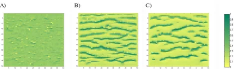
Eight simulations were performed using hydraulic con-ductivity functions obtained through Eq. (14), with coeffi-cientsAequal to:−0.4,−0.3,−0.2,−0.1, 0.1, 0.2, 0.3 and 0.4. The statistical analysis of the vegetation clusters, shown in Table 4, shows the impact that the shape of the hydraulic conductivity function has on the spatial configuration of the vegetation. As shown in Fig. 18, patterns emerge only for

Fig. 19. Effect of local plants’ interactions on pattern formation. (A) No interactions. (B) Spatially variable (function of neighbors’

vegetation and surface runoff) interactions.

climatic and soil conditions, not included in this paper). As shown in Fig. 18, the functions obtained through Eq. (14) are not significantly different from that of the base conditions, even in the two limit cases ofA= −0.4 andA=0.4. Never-theless, even these small differences have a strong impact on the system response. For example, in the case ofA= −0.4, which leads to no patterns, the PDF of the resulting vege-tation density distribution has modes atM≈0.1 (bare soil patches) andM≈0.45 (vegetated clumps). Those two val-ues ofMcorrespond to the range for which the slope of the hydraulic conductivity function of the base conditions (i.e.,

A=0) is higher than for the case A= −0.4. In the base conditions simulation, this large function gradient allows ar-eas withM≈0.4 to be sufficiently permeable to favor wa-ter infiltration and further vegetation establishment, trigger-ing the positive feedback which ultimately promotes pattern formation. In the case ofA= −0.4, instead, the soil perme-ability required to favor run-on infiltration would be reached in areas with vegetal cover M >0.7, which is too high to be sustainable, given the climatic and the hydraulic proper-ties of the system. Other simulations performed on different sets of climatic and hydraulic conditions support this find-ing and indicate that each set of climatic and hydraulic con-ditions requires the hydraulic conductivity function to have a particular shape for the vegetation configuration to be pat-terned. Specifically, the hydraulic conductivity function must be such that: (1) the permeability for low vegetated areas (e.g., M <0.2) promotes the formation of surface runoff without allowing further establishment of vegetation (and, thus, positive feedback on permeability) and (2) the vege-tated areas (e.g., M >0.4) are permeable enough to allow run-on infiltration and sustain (for the given climatic condi-tions) their vegetal coverage and/or promote further vegeta-tion establishment.

Fig. 20. Effect of soil moisture redistribution due to roots on pattern

formation. (A) No roots redistribution. (B) Roots are able to reroute the soil moisture from adjacent less vegetated areas.

5.3.4 Impact of local interactions

The effect of interactions between adjacent clumps of veg-etation was modeled, as indicated before, by allowing the transpiration efficiency of the vegetation at a certain pixel to depend on the vegetal density of the nearby pixels (see Eq. 7). We explored the effect of this spatial interaction on pattern formation by examining the evolution of the system in its absence, and comparing it with the results obtained for the base conditions, which includes it. Figure 19 shows that even in the absence of spatial interactions between plants in adjacent pixels, the system evolves towards a patterned con-figuration. However, the shape of the pattern and the total amount of vegetation arising in the domain are different in the two cases, as also evident in Fig. 22. This suggests that the net effect of the spatial interactions encoded in Eq. (8) through Eq. (12) (protection from temperature and humidity fluctuations, protection from soil erosion, protection from the mechanical damages due to winds and animals, enhancement of soil fertility through litter formation and nutrient replen-ishment and so on) is important for the ultimate configuration of patterns and total amount of biomass produced, although not essential for the emergence of the patterns themselves.

In order to investigate the individual effect of each of the interactions of Eq. (7), we carried out five simulations of the system, each one performed by setting one of the coefficients

αi of Eq. (8) through Eq. (12) equal to zero. A statistical analysis of the vegetation clusters obtained in those five cases is compared to the base conditions in Table 2. Notably, the simulation obtained withα2=0, which corresponds to the

absence of facilitation due to surrounding vegetation, does not lead to the formation of patterns, whereas all the other cases do; the emerging banded patterns are of different shape and dimension, although never in a measure that results in the transition to spots or labyrinths, at least for the set of soil–climatic conditions considered here.

5.3.5 Impact of soil moisture redistribution due to roots