Seasonal streamflow forecasts in the Ahlergaarde catchment, Denmark: the effect of preprocessing and post processing on skill and statistical consistency

https://doi.org/10.5194/hess-22-3601-2018 © Author(s) 2018. This work is distributed under the Creative Commons Attribution 4.0 License.

Seasonal streamflow forecasts in the Ahlergaarde catchment,

Denmark: the effect of preprocessing and post-processing on skill

and statistical consistency

Diana Lucatero1, Henrik Madsen2, Jens C. Refsgaard3, Jacob Kidmose3, and Karsten H. Jensen1

1_{Department of Geosciences and Natural Resource Management, University of Copenhagen, Copenhagen, Denmark} 2_{DHI, Hørsholm, Denmark}

3_{Geological Survey of Denmark and Greenland (GEUS), Copenhagen, Denmark}

Correspondence:Diana Lucatero ([email protected]) Received: 30 June 2017 – Discussion started: 12 July 2017

Revised: 23 February 2018 – Accepted: 27 May 2018 – Published: 4 July 2018

Abstract.In the present study we analyze the effect of bias adjustments in both meteorological and streamflow forecasts on the skill and statistical consistency of monthly stream-flow and yearly minimum daily stream-flow forecasts. Both raw and preprocessed meteorological seasonal forecasts from the European Centre for Medium-Range Weather Forecasts (ECMWF) are used as inputs to a spatially distributed, cou-pled surface–subsurface hydrological model based on the MIKE SHE code. Streamflow predictions are then gener-ated up to 7 months in advance. In addition to this, we post-process streamflow predictions using an empirical quan-tile mapping technique. Bias, skill and statistical consistency are the qualities evaluated throughout the forecast-generating strategies and we analyze where the different strategies fall short to improve them. ECMWF System 4-based streamflow forecasts tend to show a lower accuracy level than those gen-erated with an ensemble of historical observations, a method commonly known as ensemble streamflow prediction (ESP). This is particularly true at longer lead times, for the dry sea-son and for streamflow stations that exhibit low hydrologi-cal model errors. Biases in the mean are better removed by post-processing that in turn is reflected in the higher level of statistical consistency. However, in general, the reduction of these biases is not sufficient to ensure a higher level of ac-curacy than the ESP forecasts. This is true for both monthly mean and minimum yearly streamflow forecasts. We discuss the importance of including a better estimation of the initial state of the catchment, which may increase the capability of the system to forecast streamflow at longer leads.

1 Introduction

Seasonal streamflow forecasting encompasses a variety of methods that range from purely data-based to entirely model-based or hybrid methods that exploit the benefits of each (Mendoza et al., 2017). Data-driven methods find empiri-cal relationships between streamflow and a variety of pre-dictors. These relationships are then used to derive forecasts for the upcoming seasons. Different predictors can be used depending on the relative importance they have for the re-gional hydroclimatic conditions. Predictors that have been used include large-scale climate indicators such as El Niño or the North Atlantic Oscillation, (Schepen et al., 2016; Shamir, 2017; Wang et al., 2009; Olsson et al., 2016), pre-cipitation and land temperature (Córdoba-Machado et al., 2016), the state of the catchment in the form of streamflow, soil moisture, groundwater storages or snow storages that can be derived either by the use of a hydrological model, hence the term “hybrid” (Robertson et al., 2013; Rosenberg et al., 2011), or by means of observed antecedent conditions (Robertson and Wang, 2012).

Wood and Lettenmaier, 2006; Yuan et al., 2011, 2013, 2015, 2016). In principle, the latter should be more suitable in pro-viding skillful forecasts as they are able to capture the evolv-ing chaotic behavior of the atmosphere, whereas the ESP ap-proach assumes that what has been observed in the past can be used as a proxy for what will happen in the future, an assumption that requires stationary climate conditions. On the other hand, the lack of reliability of GCMs in forecast-ing atmospheric patterns at long lead times precludes their use in weather-impacted sectors (Bruno Soares and Dessai, 2016; Weisheimer and Palmer, 2014). For example, a previ-ous study on the skill of the European Centre for Medium-Range Weather Forecasts (ECMWF) System 4 in Denmark concluded that, in general, the precipitation forecast bias in the catchment area was in general around−25 % (Lucatero et al., 2017). This bias, together with the sharpness of forecasts, led to a mild positive skill limited to the first month lead time (Lucatero et al., 2017). These results are in accordance with skill studies with focus on a similar area (Crochemore, et al., 2017). This is the reason why preprocessing and post-processing should be performed when using GCM forecasts to force a hydrological model to eliminate biases intrinsic to climate and hydrological models. In the context of this study, preprocessing refers to any method that improves the forcings, i.e., precipitation and temperature, used in the hy-drological forecasting system. Post-processing refers to the improvements achieved in the outputs of the hydrological model, e.g., streamflow. In this respect, post-processing also corrects errors in hydrological models that cannot be elimi-nated through calibration (Shi et al., 2008; Yuan et al., 2015; Yuan and Wood, 2012).

A couple of studies have quantified the effects on stream-flow skill by preprocessing either seasonal (Crochemore et al., 2016) or medium-range (Verkade et al., 2013) forecasts. Other studies have assessed the efficiency of post-processing streamflow forecasts only (Bogner et al., 2016; Madadgar et al., 2014; Ye et al., 2015; Zhao et al., 2011; Wood and Schaake, 2008). To the best of our knowledge, only Roulin and Vannitsem (2015), Yuan and Wood (2012) and Zala-chori et al. (2012) have compared the additional gain in skill of doing both preprocessing and post-processing. The vious studies have shown that improvements made by pre-processing the forcings do not necessarily translate into im-provements in streamflow forecasts (Verkade et al., 2013; Zalachori et al., 2012). Improvements are larger when post-processing is done, and a combination of prepost-processing and post-processing provides the best results (Yuan and Wood, 2012; Zalachori et al., 2012). To the best of our knowledge, only Yuan and Wood (2012) have made this evaluation in the context of seasonal forecasting.

The present study focuses on the following aspects: (i) the evaluation of the use of a GCM to generate seasonal stream-flow forecasts, (ii) the study of the effect that preprocess-ing and post-processpreprocess-ing have on streamflow forecasts 1– 7 months ahead, and (iii) the effect of hydrological model

biases in forecast skill evaluations. This is done by a com-bination of the following methodological choices. First, we make use of seasonal meteorological forecasts of ECMWF System 4 (Molteni, et al., 2011). Secondly, the hydrological simulations use an integrated physically based and spatially distributed model based on the MIKE SHE code (Graham and Butts, 2005). Thirdly, our evaluation focuses on three forecast qualities: bias, skill and statistical consistency. Skill is measured using ESP as a reference and focusing on both accuracy and sharpness. Finally, the focus here is to evaluate forecasts of monthly average streamflow throughout the year and minimum daily flows during the summer. The catchment serving as a basis of our study is groundwater-dominated and is located in a region where seasonal forecasting is a chal-lenging endeavor (Lucatero et al., 2017). The following ques-tions are then addressed.

1. How do GCM-generated forecasts compare to those of the ESP approach?

2. What is the effect of preprocessing and post-processing on streamflow forecasts in terms of bias, skill and sta-tistical consistency? And more specifically, is there one single approach, or a combination of several, that re-duces the bias and augments skill and statistical consis-tency?

3. What is the effect that hydrological model bias has on the evaluation of preprocessed and post-processed streamflow forecasts?

2 Data and methods

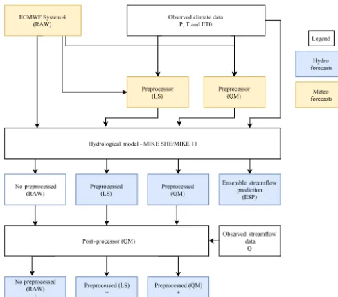
The following sections give a description of the methodol-ogy followed in this study. A graphical depiction of the steps carried out can be seen in Fig. 1.

2.1 Area of study, observational data and hydrological model

The present study is carried out for the Ahlergaarde catch-ment located in West Jutland, Denmark (Fig. 2), which has a size of 1044 km2. It is located in one of the most irrigated zones in Denmark, with 55 % of the area covered with agri-cultural crops such as barley, grass, wheat, maize and pota-toes. The remaining area is distributed in categories as fol-lows: grass (30 %), forest (7 %), heath (5 %), urban (2 %) and other (1 %) (Jensen and Illangasekare, 2011).

Figure 1.Diagram of generation of forecasts and verification proce-dures. RAW refers to the uncorrected ECMWF System 4 forecasts, while LS and QM refer to forecasts (either meteorological or hydro-logical) that are corrected using the linear scaling/delta change or quantile mapping method, respectively, for precipitation (P), tem-perature (T) and reference evapotranspiration (ET0). Preprocessed refers to streamflow forecasts generated using corrected meteoro-logical forecasts while post-processed refers to corrected stream-flow forecasts.

geological composition of the surface layer is that overland flow rarely happens (Jacob Kidmose, personal communica-tion, 2014). Daily precipitation (P), temperature (T) and ref-erence evapotranspiration (ET0) data are retrieved from the

Danish Meteorological Institute (DMI; Scharling and Kern-Hansen, 2012). The dataset spatial domain covers Denmark with a 10 km grid resolution forP and a 20 km resolution for

T andET0.P is corrected for systematic under-catch due

to wind effects (Stisen et al., 2011, 2012), and ET0 is

de-rived using the Makkink formulation (Hendriks, 2010). Fi-nally, daily streamflow observations are retrieved from the Danish Hydrological Observatory (HOBE) (Jensen and Il-langasekare, 2011) datasets.

The hydrological simulations for this study are grounded on a physically based, spatially distributed, coupled surface– subsurface model that simulates the main hydrological pro-cesses such as evapotranspiration, overland flow, unsatu-rated, saturated and streamflows and their interactions. The model is based on the MIKE SHE code (Graham and Butts, 2005). Groundwater flow is described by the governing equation for three-dimensional groundwater flow based on Darcy’s law. Drain flow is considered when the groundwater table exceeds a drain level. Surface water flow in streams is simulated by a one-dimensional channel flow model based on kinematic routing, while a two-dimensional diffusive wave approximation of the St. Venant equations is used for

over-land flow routing. Finally, a two-layer approach is used for the simulations of unsaturated flow and evapotranspiration (Graham and Butts, 2005). Snow is not an important process in the study area; therefore, the model takes snowmelt into account by using a simple degree-day model formulation. The horizontal numerical discretization is 200 m, whereas the vertical discretization is based on six numerical lay-ers whose dimension depends on the geological stratigra-phy. Model parameters were calibrated against groundwa-ter head and discharge using an automated optimizer, PEST (parameter estimation) version 11.8 (Doherty, 2016) for the 2006–2009 period. Parameters to be calibrated were selected based on a sensitivity analysis study. These are hydraulic conductivities for 10 geological units, specific yield, spe-cific storage, drain time constant, detention storage, river-groundwater conductance and root depth of 10 vegetation types. The reader is referred to Zhang et al. (2016) for fur-ther details on the calibration procedure.

2.2 Forecast generation: GCM-based and ESP

As seen in Fig. 1,P,T andET0forecasts are taken from the

ECMWF System 4 (RAW), preprocessed ECMWF System 4 (linear scaling, LS, and quantile mapping, QM), and histor-ical observations (ESP). The European Centre for Medium-Range Weather Forecasts (ECMWF) offers a seasonal fore-casting product that currently is in its version number 4 (Molteni et al., 2011). An attempt to reduce the biases in-trinsic in ECMWF System 4 led to what we refer to as pre-processed forecasts. The reader is referred to Lucatero et al. (2017) for details of the evaluation of both ECMWF Sys-tem 4 and preprocessed forecasts for Denmark. The spatial resolution of the raw forecasts is 0.7◦_{in latitude and}

longi-tude. Forecasts were interpolated to a 10 km grid to match the resolution of the observed grid. For the Ahlergaarde catch-ment, forecast–observation data for the 1990–2013 period are extracted for 24 grid points covering the study area, lead-ing to a sample size of 24 years. Finally,ET0is computed

using the Makkink formulation (Hendriks, 2010) that takes

T and incoming shortwave solar radiation from the ECMWF System 4 forecasts as inputs.

Figure 2.Location and topography of the Ahlergaarde catchment. The outlet station (82) and the upstream sub-catchment (21) are used in the study.

● ●

● ●

●

● ●

●

●

●

● ●

0 12 24 36 48 60 72 84 96 108 120

m

m m

on

th

-1

0 2 4 6 8 10 12 14 16 18 20

°C

●

P ET0 Q T

Jan Mar May Jul Sep Nov

Figure 3. Climatology of the Ahlergaarde catchment. Values for precipitation (P), reference evapotranspiration (ET0), streamflow (Q) and temperature (T) are monthly average values over the period 1990–2013.

ESP share the same hydrological initial conditions for fore-casts initiated in the same month. These are computed from a spin-up run starting in January 1990 and up until 2013. Ini-tial states are saved on the first day of each calendar month. Forecasts are then run on a daily basis up to 7 months. 2.3 Preprocessor and post-processor

Preprocessed forcings for the hydrological model were re-trieved from data of the companion paper, Lucatero et al. (2017). The authors used two well-known bias correction techniques, LS and QM. In LS the ensemble is adjusted with a scaling factor, either by multiplication (forP andET0) or

addition (T). The scaling factor is computed as the ratio or

difference between the averages of the ensemble mean and the observed mean for a specific month, lead time and loca-tion, with the sole purpose of adjusting the mean.

QM (Zhao et al., 2017) matches the quantiles of the en-semble distribution with the quantiles of the observed distri-bution in the following way:

f_k,i∗ =G−1 F fk,i, (1)

whereG and F represent the observed and the ensemble distribution functions, respectively, for forecast–observation pair i, for i=1, . . ., M, with M being the number of forecast–observation pairs.fk,irepresents ensemble member

k,k=1, . . ., N, whereN is the ensemble size andf_k,i∗ rep-resents the corrected ensemble memberk.F is an empirical distribution function trained with all ensemble members in a given month for a given lead time and location.GandF

are fitted on a leave-one-out cross-validation mode, i.e., the forecast–observation pairiis left out of the sample. For ex-ample, for a forecast of the target month April, initialized in February,F is computed using all ensemble members, com-prising 30 (days) times 23 (number of years in the training sample minus the year to be corrected), times the ensemble size of that particular month (15 or 51). The same is done for

G. Linear extrapolation is applied to approximate the values between the bins ofF andGand to map ensemble values and quantiles that are outside the training sample.

2.4 Performance metrics

The performance of raw, preprocessed and post-processed forecasts is evaluated. Our main focus is the following four qualities: bias, skill in regards to accuracy and sharpness and statistical consistency. Bias is the measure of under- or over-estimation of the mean of the ensemble in comparison with the observed values (Yapo et al., 1996):

PBias= 

   

M P

i=1 f_i

M P

i=1 yi

−1



   

·100, (2)

wheref_i andyi represent, respectively, the ensemble mean

and the observed values for forecast–observation pair i of a particular month, lead time and location. If the value in Eq. (2) is negative, we have an underprediction, and con-versely an overprediction, if the value is positive.

Secondly, we compute the continuous rank probability score CRPS (Hersbach, 2000) as a general measure of the accuracy of the forecasts. The computation of the score is as follows:

CRPS= 1

M

M X

i=1 ∞ Z

−∞

Pi(x)−H (x−yi) 2

dx, (3)

where Pi(x) represents the cumulative distribution

func-tion (CDF) of the ensemble for forecast–observafunc-tion pair

i,H (x−yi)is the Heaviside function that takes the value

0 when x < yi or 1 otherwise.yi is the verifying

observa-tion of forecast–observaobserva-tion pairi. Sharpness for forecast– observation pairiis measured as the difference between the 25 and the 75 % percentiles. The average of these differences along the forecast–observation record is then used as a mea-sure of sharpness. Both the CRPS and sharpness scores are then given in the units of the variable of interest, i.e., m−3s−1 for streamflow. Both scores are positive oriented; i.e., the lower the value, the more accurate or sharper a forecast. A skill score can then be computed in the following manner: Skill=1−Scoresys

Scoreref

, (4)

where, for the present study, Scoresysis the score of

stream-flow forecasts generated either using raw, preprocessed ECMWF System 4 or post-processed forecasts. Scoreref is

the score value of our reference system, the ESP. The range of the skill score in Eq. (4) is from−∞to 1, and values closer to 1 are preferred. Negative values indicate that, on average, the system being evaluated does not perform better than the ESP used as reference. Hereafter, we denote the skill with respect to accuracy as CRPSS and the skill in terms of sharp-ness as SS. In order to evaluate the statistical significance of the differences of skill between GCM-generated forecasts

and ESP, we use a two-sided Wilcoxon–Mann–Whitney test (WMW test) at the 5 % significance level (see Hollander et al., 2014).

Since the number of ensemble members varies from month to month, the value of the skill scores for months with a larger ensemble size will be more favorable. Although the purpose of the present study is not to make an in-depth analysis of the effect of changing ensemble size, we utilized a bootstrapping technique to make the reader aware of the possible gains in skill due to increased ensemble size. This is accomplished by computing the skill scores of a random selection of 15 of the 51 ensemble members for February, May, August and November as in Jaun et al. (2008). This step is performed 1000 times. The final value of the skill score of interest is then the average of these. Note that the bootstrapping is not applied to the ESP forecasts with an ensemble size of 23 members.

Finally, in order to evaluate the statistical consistency be-tween predictive and observed distribution functions, we use the probability integral transform (PIT) diagram. The PIT di-agram is the CDF ofzi =P (X≤yi), whereziis the value of

the cumulative distribution function that the observed value attains within the ensemble distribution for each forecast– observation pairi. Note that the PIT diagram is the continu-ous equivalent of the rank histograms (Friederichs and Tho-rarinsdottir, 2012) and it is mainly used to evaluate statistical consistency of a continuous predictive CDF. However, in this study, thez0_is are based on the empirical CDF of the ensem-ble members at a given lead time. Note that the evaluation of the appropriateness of the choice of PIT diagrams over rank histograms for ensemble forecasts is beyond the scope of the present study. For a forecasting system to be statistically con-sistent, meaning that the observations can be seen as a draw of the predictive CDF, the CDF of thez0_is should be close to the CDF of a uniform distribution in the [0, 1] range. Devia-tions from the uniform distribution signify bias in the ensem-ble mean and spread (see Laio and Tamea, 2007). Finally, in order to make the test for uniformity formal, we make use of the Kolmogorov confidence bands. The bands are two straight lines, parallel to the 1 : 1 diagonal and at a distance

q (α) /

√

M, whereq (α)is a coefficient that depends on the significance level of the test, i.e.,q (α=0.05)=1.358 (see Laio and Tamea, 2007; D’Agostino and Stephens, 1986), and

Mis again the number of forecast–observation pairs. The test for uniformity is not rejected if the CDF of thez0_is lies within these bands.

the purposes of this study, minimum daily flows are defined as the flow of the day with the minimum yearly discharge (m−3_s−1_{) that usually happens during July to September}

(Fig. 3). Note that timing errors are not an issue here due to the computation choice of minimum daily flows. Observed minimum daily flow is computed as the flow of the day with the minimum discharge over the 7-month forecasting period (April–October). Forecasted minimum daily flow (for each ensemble) is computed in the same manner. Timing errors will only be visible if forecasted minimum daily flow was chosen to be the discharge values of the day where minimum daily flow was observed, which is not the case here. Studies that have focused their attention on situations of low flow or hydrological drought in the context of seasonal forecasting exist (Fundel et al., 2013; Demirel et al., 2015; Trambauer et al., 2015), documenting the possibility of extracting skillful forecasts months ahead for low flow/drought scenarios. Fi-nally, minimum daily flow forecasts are evaluated using the same skill scores as for monthly flow forecasts, i.e., using ESP as a reference forecast.

3 Results

3.1 Hydrological model evaluation

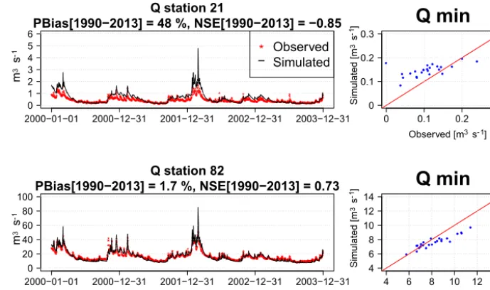
Figure 4 shows the results for simulated streamflow at the up-stream station 21 and the downup-stream station 82. The focus of the evaluation is done for daily values during the period from 2000 to 2003. As a preliminary evaluation, we com-puted the percent bias (PBias) and the Nash–Sutcliffe model efficiency coefficient (NSE) for the complete observed– simulated record (1990–2013). There is, in general, a good agreement in timing between observed and simulated values. The visual inspection of the hydrographs reveal, however, an amplitude error that is more pronounced at the upstream sta-tion 21, especially during the winter season. Evidence for this is also reflected by the high values of bias and the neg-ative NSE for this station (NSE= −0.85). Furthermore, a scatterplot of simulated and observed minimum daily flows for the 24 years shows an overestimation of the minimum daily flows that is more pronounced at the upstream station (Fig. 4). At the outlet station 82 there is a better behavior in terms of bias and NSE, with an overestimation of only 1.7 % and a NSE of 0.73. Moreover, for this station there is a better agreement in both the high and low flows through the year. The latter can be verified by looking at the scatterplot of the minimum daily flows (Fig. 4), with the majority of points lying close to the 1 : 1 diagonal.

Due to the poor performance at the upstream station 21, in the following Sect. 3.2–3.4 we will discuss the skill and consistency of the different approaches for forecast improve-ment, with a focus on the outlet station only. The large biases in the upstream station, combined with the structural biases of the meteorological forecasts, seem to inflate the skill of

the streamflow forecasts. This will be further discussed in Sect. 3.5.

3.2 Streamflow forecasts forced with raw meteorological forecasts

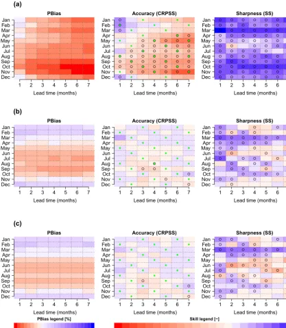
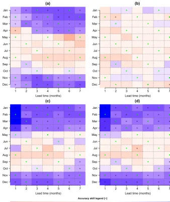
The bias and skill of the monthly streamflow forecasts forced with raw ECMWF forecasts are shown in the first row of Fig. 5. The x axis represents the different lead times in months, while theyaxis represents the target month. For ex-ample, the bias of November with a lead time of 2 represents the value of bias for a forecast initiated on 1 October for the target month of November. This bias is in the [−30,−20 %] range. In general, the absolute bias increases with lead time, and usually moves from an overprediction (or mild underpre-diction) to a large negative bias at longer lead times.

Figure 5 also shows the skill of accuracy and sharpness. The months with statistically significant differences in skill between the ESP and ECMWF System 4 forecasts are repre-sented with a black circle. There is a connection between bias and skill of accuracy in the sense that months with a higher bias tend to be the ones with lower or nonexistent skill (e.g., September, October, November). The opposite also holds; i.e., months with milder bias tend to be the months when the forecast is improving over the reference forecast to a higher degree (e.g., December, January, February). This is by no means surprising, as the CRPS penalizes forecasts that have biases.

The CRPSS is negative, except for some months during winter and at short lead times for which a forecast generated using raw ECMWF System 4 forcings improves accuracy up to 40 % compared to ESP. As for the case of bias, skill depends on lead time, reaching its most negative values for forecasts generated 7 months in advance. One important fea-ture is the high skill that a forecast generated using ECMWF raw forcings has in terms of sharpness (SS). Figure 5 shows that this quality is present in the majority of target months and lead times. Note, however, that sharpness is only a de-sirable property when biases are low. In our case study, the width of the raw forecasts is smaller than that of the ESP, indicating overconfidence when biases are high.

************************************************************** *

*********************************_{***************************************************************************************************************************************************************************************************************}********************************************************************************************************* *

***********_{************************************************************************************************************************************************************************************************************************************************************************************************************************}**************************************************** * *** * * *********************_{*******************************************************************************************}*

****************************************************************************************************************************************************************************************************************************************************************************************************************************************************************************************************************************************************************************************************************************************************************************** Q station 21

PBias[1990−2013] = 48 %, NSE[1990−2013] = −0.85

2000−01−01 2000−12−31 2001−12−31 2002−12−31 2003−12−31 0

1 2 3 4 5 6

*

− ObservedSimulated

m

3 s

-1

***************_{**************}******************************** ** ** **************

************************************************_{****************************************************************************************************************************************************************************}***** * *** * *************** ** ******************************_{*************************************************}****

** *******_{***********************************************************************************************************************************}

**************************************************************************************************************************************************************************************** **_{****************}************

*** ******************

******** ***********

*******************************_{*********************************************************************************************************************************************************}

****************************************************************************************************************************************************************************************************************************************************************************************************************************************************************************************************************************************************************************************** Q station 82

PBias[1990−2013] = 1.7 %, NSE[1990−2013] = 0.73

2000−01−01 2000−12−31 2001−12−31 2002−12−31 2003−12−31 0

20 40 60 80 100

m

3 s

-1

● ● ● ●

● ●

● ●

● ● ● ●

●

● ●● ●

● ● ●

● ● ●

●

Q min

Observed [m3 _s- 1_]

S

im

ul

at

ed

[m

3 s -1]

0 0.1 0.2 0.3 0

0.1 0.2 0.3

● ● ●●

● ●

● ● ● ●

● ●

●

● ● ● ●

●

● ● ●

● ●

● ●

Q min

Observed [m3 _s- 1_]

S

im

ul

at

ed

[m

3 s -1]

4 6 8 10 12 14 4

6 8 10 12 14

Figure 4.Hydrographs for the 2000–2003 period. Percentage bias (PBias) and Nash–Sutcliffe efficiency score (NSE) are computed using the daily observed–simulated values for the complete 1990–2013 period. The scatterplots represent the observed–simulated annual minimum daily flow values.

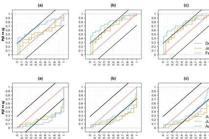
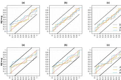
Statistical consistency of the raw forecasts is visualized on the first column of the PIT diagrams in Fig. 6 for winter (December, January and February) and summer (June, July and August) (first and second row, respectively) at a lead time of 1. Kolmogorov confidence bands are also plotted for a graphical test of uniformity at the α=0.05 level. For the sake of brevity, the remaining seasons and lead times are not shown. For the particular seasons and lead time shown, sta-tistical consistency seems to be achieved only for the wettest months (December–February). The explanation for this par-ticular behavior will be given in Sect. 3.5. Early spring and November forecasts are also able to pass the uniformity test at a lead time of 1 month (not shown). Summer forecasts to-gether with late spring and autumn months (May, September and October, not shown) show a significant underprediction, which prevents them from passing the uniformity test. Sta-tistical consistency worsens as the lead time increases, in ac-cordance with the deterioration of the bias in Fig. 5.

3.3 Streamflow forecasts forced with preprocessed meteorological forecasts

The second and third rows of Fig. 5 show the bias and skill of streamflow forecasts generated using preprocessed forcings from ECMWF System 4 using the LS and the QM method, respectively.

Several conclusions can be drawn when comparing fore-casts using the preprocessed and raw forcings. First, biases are clearly improved, especially for longer lead times. For example, for October forecasts from a lead time of 3 to 7 months, biases are reduced from the [−40, −30 %] to the [−20, 10 %] range for LS and to the [−15, 20 %] range for

QM. There are, however, no obvious differences between the two preprocessing methods, which seem to perform equally well in reducing biases. Secondly, three features of accuracy are seen. The first one is that, also for accuracy, there are no obvious differences in skill between the two preprocess-ing methods. Furthermore, there seems to be a reduction of skill for the winter months and March in the first month lead time. These months are the only ones with a statistically sig-nificant skill using the raw forecasts. This feature is a con-sequence of the reduction of the forcing biases, a situation that will be further discussed in Sect. 3.5. The last feature is that the improvement of the forcings can help to reduce the negative skill in streamflow forecasts. For example, April to November forecasts at longer lead times, generated using raw ECMWF System 4 forcings, exhibit a highly negative and statistically significant skill, sometimes lower than−1.0. Streamflow forecasts generated using preprocessed forcings for those months tend to have a neutral skill. This in turn im-plies that their accuracy is not different from the accuracy of ESP forecasts. The final conclusion is related to sharp-ness. As we can see in Fig. 5, streamflow forecasts generated using preprocessed forcings have an ensemble range that is wider than the reference ESP forecasts. This indicates that preprocessing the forcings also leads to a reduction of sharp-ness in comparison to forecasts generated using raw forcings (Sect. 3.2.).

deteriora-(a)

PBias

1 2 3 4 5 6 7

Dec NovOct Sep AugJul Jun MayApr MarFeb Jan

Lead time (months)

Accuracy (CRPSS)

1 2 3 4 5 6 7

Dec NovOct SepAug Jul Jun MayApr Mar FebJan ● ● ● ● ● ● ● ● ● ● ● ● ● ● ● ● ● ● ● ● ● ● ● ● ● ● ● ● ● ● ● ● ● ● ● ● ● ● ● ● ● ● ● ● ● ● ● ● ●

Lead time (months)

Sharpness (SS)

1 2 3 4 5 6 7

Dec NovOct SepAug Jul Jun MayApr Mar FebJan ● ● ● ● ● ● ● ● ● ● ● ● ● ● ● ● ● ● ● ● ● ● ● ● ● ● ● ● ● ● ● ● ● ● ● ● ● ● ● ● ● ● ● ● ● ● ● ● ● ● ● ● ● ● ● ● ● ● ● ● ● ● ● ● ● ● ● ● ● ● ● ● ● ● ● ● ● ● ● ● ●

Lead time (months)

(b)

PBias

1 2 3 4 5 6 7

Dec NovOct Sep AugJul Jun MayApr MarFeb Jan

Lead time (months)

Accuracy (CRPSS)

1 2 3 4 5 6 7

Dec NovOct SepAug Jul Jun MayApr Mar FebJan ● ● ● ● ● ●

Lead time (months)

Sharpness (SS)

1 2 3 4 5 6 7

Dec NovOct SepAug Jul Jun MayApr Mar FebJan ● ● ● ● ● ● ● ● ● ● ● ● ● ● ● ● ● ● ● ● ● ● ● ● ● ● ● ● ● ● ● ● ● ● ● ● ● ● ● ● ● ● ● ● ● ● ● ● ●

Lead time (months)

(c)

PBias

1 2 3 4 5 6 7

Dec NovOct Sep AugJul Jun MayApr MarFeb Jan

Lead time (months)

Accuracy (CRPSS)

1 2 3 4 5 6 7

Dec NovOct SepAug Jul Jun MayApr Mar FebJan ● ● ●

Lead time (months)

Sharpness (SS)

1 2 3 4 5 6 7

Dec NovOct SepAug Jul Jun MayApr Mar FebJan ● ● ● ● ● ● ● ● ● ● ● ● ● ● ● ● ● ● ● ● ● ● ● ● ● ● ● ● ● ● ● ● ● ● ● ● ● ● ● ● ● ● ● ● ● ●

Lead time (months) PBias legend [%]

−40 −20 0 10 20 30 40 50 60 70 80

Skill legend [−]

−1.5 −1.3 −1.1 −0.9 −0.7 −0.5 −0.3 0 0.1 0.2 0.3 0.4 0.5 0.6 0.7 0.8

Figure 5.PBias and skill in terms of accuracy and sharpness of monthly means of daily streamflow of raw and preprocessed forecasts at station 82. Streamflow forecasts are generated using (a)raw meteorological forecasts and preprocessed meteorological forecasts with the(b)linear scaling/delta change (LS) and(c)quantile mapping (QM) methods. Theyaxis represents the target month, and thexaxis represents the different lead times at which target months are forecasted. Values in the blue range show a positive bias/skill and values in red a negative bias/skill. Circles represent the cases where the distribution of the accuracy and/or sharpness for ESP differs from that of the ECMWF System 4-generated forecasts at a 5 % significance level using the WMW test. Green crosses represent the months/lead times for which the ensemble size is 51.

tion is seen for both preprocessing methods. This is caused by compensational errors that will be further discussed in Sect. 3.5. Besides that particular season, improvements in consistency after preprocessing can be seen during the au-tumn (not shown) and August, although to a lesser degree.

(a)

0

0.1 0.2 0.3 0.4 0.5 0.6 0.7 0.8 0.9 1

0 0.1 0.2 0.3 0.4 0.5 0.6 0.7 0.8 0.9 1

P(Z <= z

i

)

P(Z <= z

i

)

P(Z <= z

i

)

(b)

0

0.1 0.2 0.3 0.4 0.5 0.6 0.7 0.8 0.9 1

0 0.1 0.2 0.3 0.4 0.5 0.6 0.7 0.8 0.9 1

(c)

0

0.1 0.2 0.3 0.4 0.5 0.6 0.7 0.8 0.9 1

0 0.1 0.2 0.3 0.4 0.5 0.6 0.7 0.8 0.9 1

Dec Jan Feb

(a)

0

0.1 0.2 0.3 0.4 0.5 0.6 0.7 0.8 0.9 1

0 0.1 0.2 0.3 0.4 0.5 0.6 0.7 0.8 0.9 1

P(Z <= z

i

)

zi

P(Z <= z

i

)

zi

P(Z <= z

i

)

zi

(b)

0

0.1 0.2 0.3 0.4 0.5 0.6 0.7 0.8 0.9 1

0 0.1 0.2 0.3 0.4 0.5 0.6 0.7 0.8 0.9 1

zi

zi

zi

(c)

0

0.1 0.2 0.3 0.4 0.5 0.6 0.7 0.8 0.9 1

0 0.1 0.2 0.3 0.4 0.5 0.6 0.7 0.8 0.9 1

zi

zi

zi

Jun Jul Aug

Figure 6.PIT diagrams of monthly means of daily streamflow forecasts for winter (upper row) and summer (bottom row) of station 82 for(a)raw meteorological forecasts and preprocessed meteorological forecasts with(b)linear scaling/delta change (LS) and(c)quantile mapping (QM). The lead time is 1 month. Different colors represent different months in the season. The black lines parallel to the 1 : 1 diagonal are the Kolmogorov bands at the 5 % significance level.

3.4 Post-processed streamflow forecasts

The final step in the analysis is the post-processing of streamflow forecasts generated using raw and preprocessed ECMWF System 4 forcings. Figure 7 shows the verification results that can be directly compared to the results in Fig. 5.

The first column in Fig. 7 shows a clear reduction of the absolute bias compared to the raw and preprocessed gen-erated forecasts. Bias lies within the range [−10, 10 %], for all months and lead times. Furthermore, the majority of the CRPSS values for all months and lead times are posi-tive, while a small negative skill is seen during the autumn. Note, however, that the differences in accuracy between ESP and the post-processed forecasts are only significant at the 5 % level for few target months and lead times. In gen-eral, there seems to be a worsening of the sharpness after post-processing (Fig. 5). However, this deterioration is lower when comparing preprocessed versus post-processed fore-casts. Furthermore, the degree of the deterioration varies ac-cording to the target month. For example, summer months (June and July) exhibit a larger deterioration of sharpness; i.e., the forecast spread is larger than that of the ESP. On the other hand, forecasts for late autumn and early December ap-pear to be narrower than ESP forecasts after post-processing.

Figure 8 shows the PIT diagrams for the months of the summer and winter seasons in the first month lead time of post-processed streamflow forecasts. The plot can be directly compared to Fig. 6. As seen from the PIT diagram, all months in those seasons pass the uniformity test, indicating that af-ter post-processing, the observations can be considered as random samples of the predictive distribution. The remain-ing PIT diagrams for sprremain-ing and autumn and lead times of 2–7 months (not shown in Fig. 8) show that statistical con-sistency is present for all months and lead times. At longer lead times, the CDFs of thez_i0s are closer to the 1 : 1 diag-onal. This is achieved due to two factors: (i) the additional reduction of bias after post-processing and (ii) the worsening of sharpness for long lead times, when the larger ensemble spread encloses a larger portion of observed values.

3.5 Effect of hydrological model bias in skill evaluations

(a)

PBias

1 2 3 4 5 6 7

Dec NovOct Sep AugJul Jun MayApr Mar FebJan

Lead time (months)

Accuracy (CRPSS)

1 2 3 4 5 6 7

Dec NovOct Sep AugJul Jun MayApr MarFeb Jan ● ● ● ● ●

Lead time (months)

Sharpness (SS)

1 2 3 4 5 6 7

Dec NovOct Sep AugJul Jun MayApr Mar FebJan ● ● ● ● ● ● ● ● ● ● ● ● ● ● ● ● ● ● ● ● ● ● ● ● ● ● ● ● ● ● ● ● ● ● ● ● ● ● ● ● ● ● ● ● ● ● ● ● ● ● ● ● ● ● ● ● ● ● ● ● ● ● ● ● ●

Lead time (months)

(b)

PBias

1 2 3 4 5 6 7

Dec NovOct Sep AugJul Jun MayApr Mar FebJan

Lead time (months)

Accuracy (CRPSS)

1 2 3 4 5 6 7

Dec NovOct Sep AugJul Jun MayApr MarFeb Jan ● ● ●

Lead time (months)

Sharpness (SS)

1 2 3 4 5 6 7

Dec NovOct Sep AugJul Jun MayApr Mar FebJan ● ● ● ● ● ● ● ● ● ● ● ● ● ● ● ● ● ● ● ● ● ● ● ● ● ● ● ● ● ● ● ● ● ● ● ● ● ● ● ● ● ● ● ● ● ● ● ● ● ● ● ● ● ● ● ● ● ● ● ● ●

Lead time (months)

(c)

PBias

1 2 3 4 5 6 7

Dec NovOct Sep AugJul Jun MayApr Mar FebJan

Lead time (months)

Accuracy (CRPSS)

1 2 3 4 5 6 7

Dec NovOct Sep AugJul Jun MayApr MarFeb Jan ● ●

Lead time (months)

Sharpness (SS)

1 2 3 4 5 6 7

Dec NovOct Sep AugJul Jun MayApr Mar FebJan ● ● ● ● ● ● ● ● ● ● ● ● ● ● ● ● ● ● ● ● ● ● ● ● ● ● ● ● ● ● ● ● ● ● ● ● ● ● ● ● ● ● ● ● ● ● ● ● ● ● ● ● ● ● ● ● ● ● ● ●

Lead time (months) PBias legend [%]

−40 −20 0 10 20 30 40 50 60 70 80

Skill legend [−]

−1.5 −1.3 −1.1 −0.9 −0.7 −0.5 −0.3 0 0.1 0.2 0.3 0.4 0.5 0.6 0.7 0.8

Figure 7.PBias and skill (sharpness and accuracy) of daily monthly mean streamflow forecasts for post-processed forecasts using the quantile mapping (QM) method for predictions generated using raw(a)and preprocessed meteorological forcings with the linear scaling/delta change (b)and quantile mapping(c)methods. Legend is the same as Fig. 5. Green crosses represent the months/lead times were the ensemble size is 51.

station 21 with a large bias (PBias=48 %, Fig. 4) and sta-tion 82 with a small bias (PBias=1.7 %, Fig. 4). The figure shows CRPSS for forecasts generated using raw ECMWF forcings and preprocessed forcings with the LS method for the target months January–December at a lead time of 4 (e.g., January forecasts initiated in October). In addition to the computation of bias and accuracy of ECMWF-based stream-flow forecasts and ESP forecasts using observed streamstream-flow, we also include a computation of bias and accuracy against simulated streamflows (continuous run of the Ahlergaarde

model with observed meteorological forcings, Fig. 4). This is done in order to remove the effect of hydrological model bias and hence focus the analyses on the biases coming from forcings alone.

(a)

0

0.1 0.2 0.3 0.4 0.5 0.6 0.7 0.8 0.9 1

0 0.1 0.2 0.3 0.4 0.5 0.6 0.7 0.8 0.9 1

P(Z <= z

i

)

P(Z <= z

i

)

P(Z <= z

i

)

(b)

0

0.1 0.2 0.3 0.4 0.5 0.6 0.7 0.8 0.9 1

0 0.1 0.2 0.3 0.4 0.5 0.6 0.7 0.8 0.9 1

(c)

0

0.1 0.2 0.3 0.4 0.5 0.6 0.7 0.8 0.9 1

0 0.1 0.2 0.3 0.4 0.5 0.6 0.7 0.8 0.9 1

Dec Jan Feb

(a)

0

0.1 0.2 0.3 0.4 0.5 0.6 0.7 0.8 0.9 1

0 0.1 0.2 0.3 0.4 0.5 0.6 0.7 0.8 0.9 1

P(Z <= z

i

)

zi

P(Z <= z

i

)

zi

P(Z <= z

i

)

zi

(b)

0

0.1 0.2 0.3 0.4 0.5 0.6 0.7 0.8 0.9 1

0 0.1 0.2 0.3 0.4 0.5 0.6 0.7 0.8 0.9 1

zi

zi

zi

(c)

0

0.1 0.2 0.3 0.4 0.5 0.6 0.7 0.8 0.9 1

0 0.1 0.2 0.3 0.4 0.5 0.6 0.7 0.8 0.9 1

zi

zi

zi

Jun Jul Aug

Figure 8.PIT diagrams of daily monthly mean streamflow post-processed forecasts for summer (upper row) and winter (bottom row) of station 82. Streamflow forecasts are post-processed using the quantile mapping (QM) method for predictions generated using raw(a)and preprocessed forcings with the linear scaling/delta change(b)and quantile mapping(c)methods. Lead time 1 month. The black lines parallel to the 1 : 1 diagonal are the Kolmogorov bands at the 5 % significance level.

streamflows is also seen at station 82 for December–March, although to a lesser extent (Fig. 9b). To illustrate why this happens, Fig. 9c and d show the monthly streamflow fore-casts for all 24 years for the target month of December of forecasts initialized in September (lead time 4). Both ESP and raw (Fig. 9c) and preprocessed (Fig. 9d) forecasts are shown, along with their respective skill scores of accuracy, when the comparison is made against observed (CRPSS) and simulated (CRPSS.s) values.

Figure 9c shows two issues. First, the large hydrological model bias causes ESP to have a deviation from the obser-vations, leading to a high CRPS for the reference forecast in Eq. (4). Secondly, for the winter months, precipitation from the raw ECMWF System 4 forecasts exhibits a nega-tive bias of around−25 % (Lucatero et al., 2017). This com-pensates the biased streamflow forecasts and results in a low CRPSSys value in Eq. (4). The CRPSS then becomes

posi-tive and large (0.54). However, when the comparison is done against simulated values, the skill score becomes highly neg-ative (CRPSS.s= −0.41). Once the biases in the forcings are removed (Fig. 9d), then the hydrological model bias takes over, leading these forecasts to the same level as the ESP, increasing its CRPS, which in turn reduces the skill score (CRPSS= −0.04).

Note that the opposite situation arises, i.e., “the wrong forecast for the wrong reason”, when the hydrological model error is small and precipitation forecast bias is large. Biases in precipitation forecasts will propagate through streamflow forecasts, leading to a streamflow bias of equal sign and of similar magnitude as the precipitation bias. The streamflow bias is then reduced when the meteorological forecast bias is removed (Fig. 5, second and third row). This situation ap-pears during summer or autumn (Fig. 5, first row), when hy-drological model errors are smaller than in winter.

Station 21

● _● ● ●

● ●

● ●

● ●

● ● ● ● ●

● ●

● ● ● ●

● ●

●

(a)

Jan Feb Mar Apr May Jun Jul Aug Sep Oct Nov Dec

−0.7 −0.6 −0.5 −0.4 −0.3 −0.2 −0.1 0 0.1 0.2 0.3 0.4 0.5 0.6

CRPSS

Target month

Station 82

●

● ● ● ●

● ●

●

● ●

● ● ●

● ●

● ● ●

● ●

● ●

● _●

(b)

Jan Feb Mar Apr May Jun Jul Aug Sep Oct Nov Dec

Target month

● ● Raw vs. obs Raw vs. sim

LS vs. obs LS vs. sim

Station 21

RAW CRPSS = 0.54 CRPSS.s = −0.41

● ●

● ● ●

● ● ●

● ●

● ● ● ●

● ●

●

● ●

● ●

● ● ●

●

● ●

● ●

● ●

● ●

●

●

● ●

● ●

● ●

● ●

●

●

● ●

(c)

90 92 94 96 98 00 02 04 06 08 10 12

0 0.5 1 1.5 2 2.5 3

m

3 s

-1

Year

Station 21

LS CRPSS = −0.04 CRPSS.s = −0.05

● ●

● ● ●

● ● ●

● ●

● ● ● ●

● ●

●

● ●

● ●

● ● ●

●

● ●

● ●

● ●

● ●

●

●

● ●

● ●

● ●

● ●

●

●

● ●

(d)

90 92 94 96 98 00 02 04 06 08 10 12

● ● (c) RAW or (d) LS

ESP ObservedSimulated

Year

Figure 9. (a, b)Skill of accuracy (CRPSS) for upstream station 21 and outlet station 82 for target months January–December at a lead time of 4. Triangles and circles represent the forecasts generated using raw ECMWF System 4 forcings and preprocessed with LS, respectively, whereas black and blue lines represent the comparison against observed and simulated streamflow, respectively. The second row shows the monthly forecasts of December streamflow initialized in September (4-month lead time) for predictions using raw(c)and preprocessed (d)forcings for all years in the record (1990–2013) for station 21.

Stations like 21 could benefit the most from post-processing, removing hydrological model biases that calibra-tion alone could not remove. This is illustrated with the visu-alization of the CRPSS of the different forecasts in Fig. 10a– d. The comparison is made against observations. Figure 10b shows a reduction of skill after raw forcings have been pre-processed, as a result of the compensation errors discussed above. However, once the hydrological biases are removed with post-processing (Fig. 10c and d), the skill is positive and significant throughout November to April. Note, how-ever, that the high skill at this particular station is mainly driven by the poor performance of the reference ESP, due to the large bias of the hydrological model (Fig. 4). It is also worth noting the lack of differences in skill between Fig. 10c and d, showing that, for this particular location, a combina-tion of preprocessing plus post-processing is just as good as post-processing of the forecasts generated using raw forcings alone.

(a)

1 2 3 4 5 6 7

Dec Nov Oct Sep Aug Jul Jun May Apr Mar Feb

Jan ●

●

●

●

●

● ●

●

●

●

● ●

●

●

●

●

● ●

●

●

●

●

● ●

●

●

●

●

● ●

●

●

●

●

● ●

●

●

●

●

●

Lead time (months)

(b)

1 2 3 4 5 6 7

Dec Nov Oct Sep Aug Jul Jun May Apr Mar Feb Jan

●

●

●

●

●

Lead time (months) (c)

1 2 3 4 5 6 7

Dec Nov Oct Sep Aug Jul Jun May Apr Mar Feb

Jan ●

●

●

●

●

● ●

●

●

●

●

● ●

●

●

●

●

● ●

●

●

●

●

●

● ●

●

●

●

●

● ●

●

●

●

●

● ●

●

●

●

●

●

●

●

Lead time (months)

(d)

1 2 3 4 5 6 7

Dec Nov Oct Sep Aug Jul Jun May Apr Mar Feb Jan ●

●

●

●

●

● ●

●

●

●

●

● ●

●

●

●

●

● ●

●

●

●

●

●

● ●

●

●

●

●

● ●

●

●

●

●

● ●

●

●

●

●

●

●

●

e

L ad time (months) Accuracy skill legend [−]

−1.5 −1.4 −1.3 −1.2 −1.1 −1 −0.9 −0.8 −0.7 −0.6 −0.5 −0.4 −0.3 −0.2 0 0.1 0.2 0.3 0.4 0.5 0.6 0.7 0.8

Figure 10.CRPSS of station 21 for forecasts generated using raw (a)and preprocessed(b) forcings, in addition to the post-processed streamflow forecasts using the quantile mapping method (QM) for raw meteorological(c)and preprocessed meteorological forcings using the linear scaling/delta change method(d).

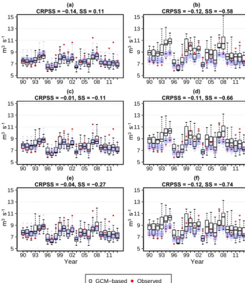
manage to perform better than ESP in terms of skill of accu-racy (CRPSS= −0.14); i.e., they are overconfident.

Preprocessing meteorological forecasts seems to have a positive effect on minimum daily flow forecasting, reducing the CRPSS from−0.14 to−0.01 when using the LS prepro-cessor. This happens because of the loss of sharpness (from 0.11 to−0.11), which allows the forecasts to better capture the higher minimum daily flows during the 00s. However, it is still difficult to outperform the ESP. Post-processing seems to have a similar effect: a loss of sharpness and de-crease in bias that allow the forecasts to capture the high minimum daily flows in the 2000s and 2010s. This situa-tion, however, leads to a loss in skill in forecasting mini-mum daily flows in the 1990s, leveling out the skill to a sim-ilar score (CRPSS= −0.12) as the forecasts generated using

raw ECMWF forcings (CRPSS= −0.14). Thus, it seems that an attempt to reduce meteorological and hydrological biases through processing the forcings and/or the streamflow will result in only a modest increase in skill of minimum daily flow predictions on average. ESP remains a reference fore-cast system difficult to outperform.

4 Discussion

(a) CRPSS = −0.14, SS = 0.11

● ● ●● ● ● ● ● ● ● ● ● ● ● ● ● ● ● ● ● ● ● ● ●

90 93 96 99 02 05 08 11

5 7 9 11 13 15 m

3 s

-1

(b) CRPSS = −0.12, SS = −0.58

● ● ●● ● ● ● ● ● ● ● ● ● ● ● ● ● ● ● ● ● ● ● ●

90 93 96 99 02 05 08 11

5 7 9 11 13 15 (c) CRPSS = −0.01, SS = −0.11

● ● ●● ● ● ● ● ● ● ● ● ● ● ● ● ● ● ● ● ● ● ● ● m

3 s

-1

90 93 96 99 02 05 08 11

5 7 9 11 13 15 (d) CRPSS = −0.11, SS = −0.66

● ● ●● ● ● ● ● ● ● ● ● ● ● ● ● ● ● ● ● ● ● ● ●

90 93 96 99 02 05 08 11

5 7 9 11 13 15 (e) CRPSS = −0.04, SS = −0.27

● ● ●● ● ● ● ● ● ● ● ● ● ● ● ● ● ● ● ● ● ● ● ● Year m

3 s

-1

90 93 96 99 02 05 08 11

5 7 9 11 13 15 (f) CRPSS = −0.12, SS = −0.74

● ● ●● ● ● ● ● ● ● ● ● ● ● ● ● ● ● ● ● ● ● ● ● Year

90 93 96 99 02 05 08 11

5 7 9 11 13 15 ● GCM−based ESP Observed m 3s -1 m 3s -1 m 3s -1

Figure 11.Forecasts of minimum daily flows for each year of the period 1990–2013, considering a forecast issued on 1 April for the next 7 months. Forecasts are generated using raw forcings(a), pre-processed forcings with the linear scaling/delta change(c)and the quantile mapping(e)methods and post-processed streamflow for forecasts generated using raw(b)and preprocessed inputs (dandf). Blue shaded box plots are ESP forecasts. CRPSS and SS are com-puted using Eq. (4) with ESP as reference.

in Wood et al. (2005), Yuan et al. (2013) and, more recently, Crochemore et al. (2016) for France. GCM-based streamflow forecasts could then be of potential use if the end user is in-terested in gaining accuracy of forecasts for the next month only. Moreover, we were able to demonstrate that, at least for a groundwater-dominated catchment located in a region with temperate climate, the GCM ability to improve forecasts of minimum daily flows within a year is also limited, regard-less of any attempts to correct forcings and/or streamflow forecasts. Further research could focus on the usefulness of GCM forecasts for drought forecasting, i.e., magnitude, du-ration and severity (Fundel, 2013) in comparison to forecasts generated using the ESP method.

Furthermore, caution must be taken when hydrological model errors are large, as it may lead to erroneous eval-uations of skill when hydrological model biases are neu-tralized by opposite GCM errors, e.g., forecasts of monthly streamflow during the winter in the study region. This is an issue somewhat underexplored in studies of forecast skill and should be evaluated especially when calibration objec-tive functions focus on attributes that differ from the ones

looked for in the final forecast quantity of interest, and when no attempts to remove biases in meteorological forecasts are made.

In our study, preprocessing of the forcings alone helped to reduce streamflow biases and reduce the negative skill at longer lead times. The reduction of the under- or over-estimation led to forecasts with a higher statistical consis-tency for most of the months and lead times considered. This rather mild enhancement was also found by Crochemore et al. (2016). Moreover, post-processing alone does a better job in removing biases in the mean, which, in turn, helps to ame-liorate issues with the statistical consistency. Ye et al. (2015) and Zalachori et al. (2012) also report the above behavior, whereas Yuan and Wood (2012) found a better correction of statistical consistency after both preprocessing and post-processing. The removal of biases of both forcings and hy-drological model did not ensure a higher level of accuracy than the ESP, as demonstrated by the nonsignificant differ-ences of accuracy between GCM-based forecasts and the ESP forecasts. This is also true for forecasts of minimum daily flows in a year, as mentioned above.

The methods used here for preprocessing (LS and QM) and post-processing (QM) were chosen because of their sim-plicity. However, post-processing in general is a field that has been gaining traction over the last decade, with a variety of methods that differ in their mathematical sophistication. The reader is referred to Li et al. (2017) for a detailed and up-dated literature review on the subject. Moreover, QM disad-vantages have been widely discussed in Zhao et al. (2017) and references therein. The main issue discussed concerns the fact that when the forecast–observation linear relation-ship is weak, or nonexistent, QM has difficulties creating forecasts that are consistent (i.e., that have skill at least as good as the reference forecast). Other methods could have been used that allow for correction of both statistical consis-tency together with consisconsis-tency. However, the benefits of the more sophisticated methods might be dampened due to the limited sample size, which is often the case in hydrometeo-rological forecasting. Nevertheless, our present study could be extended by analyzing the added skill gained by the in-creased complexity of processing methods, using the same reforecast dataset, such as the case of Mendoza et al. (2017), although with its application focused on statistical forecast-ing.

This correlation can be further explored in the forecasting mode to extend the positive skill lead time by means of data assimilation (Zhang et al., 2016) or by statistical post-processing of streamflow forecasts (Mendoza et al., 2017). Moreover, predictability attribution studies exist that quan-tify the sensitivity of the skill of a forecasting system relative to different degrees of uncertainty, either in the forcing or the initial conditions. Wood et al. (2016) developed a framework to detect where to concentrate on improvements, e.g., either the initial conditions, usually by means of data assimilation (Zhang et al., 2016), or the seasonal climate forecasts. This might shed light on, and possibly reinforce, the hypothesis that for groundwater-dominated catchments and forecasting of low flows, initial conditions will have a higher influence on forecast skill at longer lead times (Paiva et al., 2012; Fun-del et al., 2013).

5 Conclusions

Seasonal forecasts of streamflows initiated in each calen-dar month for the 1990–2013 period were generated for a groundwater-dominated catchment located in a region where seasonal atmospheric forecasting is a challenge. We analyzed the bias and statistical consistency of monthly streamflow forecasts forced with ECMWF System 4 seasonal forecasts along all calendar months throughout the year. In addition to this, we evaluated their accuracy and sharpness relative to that of the forecasts generated using an ensemble of historical meteorological observations, the ESP. Monthly streamflow forecasts generated using raw ECMWF System 4 forcings show skill only during the winter months in the first month lead time. Nevertheless, it was shown that the apparent large skill can be an effect of compensational errors between me-teorological forecasts and the hydrological model. Due to bi-ases of GCM-based meteorological seasonal forecasts and errors in the hydrological model that calibration alone can-not defuse, both preprocessing and post-processing using two popular and simple correction techniques were used to remove them: LS and QM. Finally, we also estimated the skill that the different forecast generation approaches have on forecasting the minimum yearly daily discharge. Our results show that post-processing streamflow allows for the most gain in skill and statistical consistency. However, monthly streamflow and annual minimum daily discharge forecasts generated using forcings from GCM still show difficulties in outperforming ESP forecasts, especially at lead times longer than 1 month.

Data availability. ECMWF seasonal reforecasts are available un-der a range of licences; for more information visit http://www. ecmwf.int (last access: 27 June 2018). The hydrological model forcing data (temperature, precipitation and reference evapotran-spiration) are from the Danish Meteorological Institute (https:// www.dmi.dk/vejr/arkiver/vejrarkiv/, last access: 27 June 2018). The

streamflow data are available on the HOBE data platform (http:// www.hobe.dk/index.php/data/live-data, last access: 27 June 2018). A more detailed description of the data usage can be found on the Hydrocast project website (http://hydrocast.dhigroup.com/, last ac-cess: 27 June 2018) and the HOBE project website (http://hobe.dk/, last access: 27 June 2018).

Competing interests. The authors declare that they have no conflict of interest.

Special issue statement. This article is part of the special issue “Sub-seasonal to seasonal hydrological forecasting”. It is not as-sociated with a conference.

Acknowledgements. This study was supported by the project “HydroCast – Hydrological Forecasting and Data Assimilation”, contract no. 0603-00466B (http://hydrocast.dhigroup.com/, 27 June 2018), funded by the Innovation Fund Denmark. Special thanks to Florian Pappenberger for providing the ECMWF System 4 reforecast and Andy Wood and Pablo Mendoza for hosting the first author at NCAR. We also express our gratitude to Massimiliano Zappa and one anonymous reviewer for their comments that improved the quality of this paper.

Edited by: Maria-Helena Ramos

Reviewed by: Massimiliano Zappa and one anonymous referee

References

Bogner, K., Liechti, K., and Zappa, M.: Post-processing of stream flows in Switzerland with an emphasis on low flows and floods, Water (Switzerland), 8, 115, https://doi.org/10.3390/w8040115, 2016.

Bruno Soares, M. and Dessai, S.: Barriers and enablers to the use of seasonal climate forecasts amongst organisations in Europe, Clim. Change, 137, 89–103, https://doi.org/10.1007/s10584-016-1671-8, 2016.

Córdoba-Machado, S., Palomino-Lemus, R., Gámiz-Fortis, S. R., Castro-Díez, Y., and Esteban-Parra, M. J.: Sea-sonal streamflow prediction in Colombia using atmo-spheric and oceanic patterns, J. Hydrol., 538, 1–12, https://doi.org/10.1016/j.jhydrol.2016.04.003, 2016.

Crochemore, L., Ramos, M.-H., and Pappenberger, F.: Bias cor-recting precipitation forecasts to improve the skill of seasonal streamflow forecasts, Hydrol. Earth Syst. Sci., 20, 3601–3618, https://doi.org/10.5194/hess-20-3601-2016, 2016.

D’Agostino, R. B. and Stephens, A. M.: Goodness-of-fit techniques, Dekker, New York, 1986.

Day, G. N.: Extended stream flow forecasting Using NWSRFS, J. Water Res. Pl., 111, 157–170, 1985.

Doherty, J.: PEST, Model-independent parameter estimation, User manual: 5th Edn., Watermark Numerical Computing, 2010. Friederichs, P. and Thorarinsdottir, T. L.: Forecast verification

for extreme value distributions with an application to prob-abilistic peak wind prediction, Environmetrics, 23, 579–594, https://doi.org/10.1002/env.2176, 2012.

Fundel, F., Jörg-Hess, S., and Zappa, M.: Monthly hydrometeoro-logical ensemble prediction of streamflow droughts and corre-sponding drought indices, Hydrol. Earth Syst. Sci., 17, 395–407, https://doi.org/10.5194/hess-17-395-2013, 2013.

Graham, D. N. and Butts, M. B.: Flexible, integrated watershed modelling with MIKE SHE, in: Watershed Models, edited by: Singh, V. P. and Frevert D. K., 245–272, CRC Press, Florida, 2005.

Hendriks, M.: Introduction to Physical Hydrology, Oxford Univer-sity Press, Oxford, 2010.

Hersbach, H.: Decomposition of the Continuous Ranked Prob-ability Score for Ensemble Prediction Systems, Weather Forecast., 15, 559–570, https://doi.org/10.1175/1520-0434(2000)015<0559:DOTCRP>2.0.CO;2, 2000.

Hollander, M., Wolfe, D. A., and Chicken, E.: Nonparametric statis-tical methods, 3 Edn., Wiley Series in Probability and Statistics, Hoboken, New Jersey, 2014.

Jaun, S., Ahrens, B., Walser, A., Ewen, T., and Schär, C.: A probabilistic view on the August 2005 floods in the upper Rhine catchment, Nat. Hazards Earth Syst. Sci., 8, 281–291, https://doi.org/10.5194/nhess-8-281-2008, 2008.

Jensen, K. H. and Illangasekare, T. H.: HOBE: A

Hy-drological Observatory, Vadose Zone J., 10, 1–7,

https://doi.org/10.2136/vzj2011.0006, 2011.

Laio, F. and Tamea, S.: Verification tools for probabilistic fore-casts of continuous hydrological variables, Hydrol. Earth Syst. Sci., 11, 1267–1277, https://doi.org/10.5194/hess-11-1267-2007, 2007.

Li, W., Duan, Q., Miao, C., Ye, A., Gong, W., and Di, Z.: A review on statistical postprocessing methods for hydrom-eteorological ensemble forecasting, WIREs Water, 4, e1246, https://doi.org/10.1002/wat2.1246, 2017.

Lucatero, D., Madsen, H., Refsgaard, J. C., Kidmose, J., and Jensen, K. H.: On the skill of raw and postprocessed ensemble sea-sonal meteorological forecasts in Denmark, Hydrol. Earth Syst. Sci. Discuss., https://doi.org/10.5194/hess-2017-366, in review, 2017.

Madadgar, S., Moradkhani, H., and Garen, D.: Towards improved post-processing of hydrologic forecast ensembles, Hydrol. Pro-cess., 28, 104–122, https://doi.org/10.1002/hyp.9562, 2014. Mendoza, P. A., Wood, A. W., Clark, E., Rothwell, E., Clark, M.

P., Nijssen, B., Brekke, L. D., and Arnold, J. R.: An inter-comparison of approaches for improving operational seasonal streamflow forecasts, Hydrol. Earth Syst. Sci., 21, 3915–3935, https://doi.org/10.5194/hess-21-3915-2017, 2017.

Molteni, F., Stockdale, T., Balmaseda, M., Balsamo, G., Buizza, R., Ferranti, L., Magnusson, L., Mogensen, K., Palmer, T., and Vi-tart, F.: The new ECMWF seasonal forecast system (System 4), ECMWF Technical Memorandum 656, November, 49, 2011. Olsson, J., Uvo, C. B., Foster, K., and Yang, W.: Technical Note:

Initial assessment of a multi-method approach to spring-flood forecasting in Sweden, Hydrol. Earth Syst. Sci., 20, 659–667, https://doi.org/10.5194/hess-20-659-2016, 2016.

Paiva, R. C. D., Collischonn, W., Bonnet, M. P., and de Gonçalves, L. G. G.: On the sources of hydrological prediction uncer-tainty in the Amazon, Hydrol. Earth Syst. Sci., 16, 3127–3137, https://doi.org/10.5194/hess-16-3127-2012, 2012.

Robertson, D. E. and Wang, Q. J.: A Bayesian Approach to Pre-dictor Selection for Seasonal Streamflow Forecasting, J. Hy-drometeorol., 13, 155–171, https://doi.org/10.1175/JHM-D-10-05009.1, 2012.

Robertson, D. E., Pokhrel, P., and Wang, Q. J.: Improving statistical forecasts of seasonal streamflows using hydrolog-ical model output, Hydrol. Earth Syst. Sci., 17, 579–593, https://doi.org/10.5194/hess-17-579-2013, 2013.

Rosenberg, E. A., Wood, A. W., and Steinemann, A. C.: Sta-tistical applications of physically based hydrologic models to seasonal streamflow forecasts, Water Resour. Res., 47, 3, https://doi.org/10.1029/2010WR010101, 2011.

Roulin, E. and Vannitsem, S.: Post-processing of medium-range probabilistic hydrological forecasting: Impact of forcing, initial conditions and model errors, Hydrol. Process., 29, 1434–1449, https://doi.org/10.1002/hyp.10259, 2015.

Scharling, M. and Kern-Hansen, C.: Climate Grid Denmark – Date-set for use in research and education, DMI Tech. Rep., 1–12, available at: https://www.dmi.dk/vejr/arkiver/vejrarkiv/ (last ac-cess: 27 June 2018), 2012.

Schepen, A., Zhao, T., Wang, Q. J., Zhou, S., and Feikema, P.: Op-timising seasonal streamflow forecast lead time for operational decision making in Australia, Hydrol. Earth Syst. Sci., 20, 4117– 4128, https://doi.org/10.5194/hess-20-4117-2016, 2016. Shamir, E.: The value and skill of seasonal forecasts for

wa-ter resources management in the Upper Santa Cruz River basin, southern Arizona, J. Arid Environ., 137, 35–45, https://doi.org/10.1016/j.jaridenv.2016.10.011, 2017.

Shi, X., Wood, A. W., and Lettenmaier, D. P.: How Essen-tial is Hydrologic Model Calibration to Seasonal Stream-flow Forecasting?, J. Hydrometeorol., 9, 1350–1363, https://doi.org/10.1175/2008JHM1001.1, 2008.

Stisen, S., Sonnenborg, T. O., Højberg, A. L., Troldborg, L., and Refsgaard, J. C.: Evaluation of Climate Input Biases and Water Balance Issues Using a Coupled Surface-Subsurface Model, Va-dose Zone J., 10, 37–53, https://doi.org/10.2136/vzj2010.0001, 2011.

Stisen, S., Højberg, A. L., Troldborg, L., Refsgaard, J. C., Chris-tensen, B. S. B., Olsen, M., and Henriksen, H. J.: On the impor-tance of appropriate precipitation gauge catch correction for hy-drological modelling at mid to high latitudes, Hydrol. Earth Syst. Sci., 16, 4157–4176, https://doi.org/10.5194/hess-16-4157-2012, 2012.

Trambauer, P., Werner, M., Winsemius, H. C., Maskey, S., Dutra, E., and Uhlenbrook, S.: Hydrological drought fore-casting and skill assessment for the Limpopo River basin, southern Africa, Hydrol. Earth Syst. Sci., 19, 1695–1711, https://doi.org/10.5194/hess-19-1695-2015, 2015.

Verkade, J. S., Brown, J. D., Reggiani, P., and Weerts, A. H.: Post-processing ECMWF precipitation and temper-ature ensemble reforecasts for operational hydrologic fore-casting at various spatial scales, J. Hydrol., 501, 73–91, https://doi.org/10.1016/j.jhydrol.2013.07.039, 2013.